Gaseous infall triggering starbursts in simulated dwarf galaxies

Abstract

Using computer simulations, we explored gaseous infall as a possible explanation for the starburst phase in Blue Compact Dwarf galaxies. We simulate a cloud impact by merging a spherical gas cloud into an isolated dwarf galaxy. We investigated which conditions were favourable for triggering a burst and found that the orbit and the mass of the gas cloud play an important role. We discuss the metallicity, the kinematical properties, the internal dynamics and the gas, stellar and dark matter distribution of the simulations during a starburst. We find that these are in good agreement with observations and depending on the set-up (e.g. rotation of the host galaxy, radius of the gas cloud), our bursting galaxies can have qualitatively very different properties. Our simulations offer insight in how starbursts start and evolve. Based on this, we propose what postburst dwarf galaxies will look like.

1 Introduction

Blue Compact Dwarfs (BCDs) are dwarf galaxies which are currently undergoing an intense period of star formation. The exact classification requirements for a dwarf galaxy to be a BCD differ from author to author. Zwicky (1964) first coined the term compact, in order to classify objects that could only just be distinguished from stars on photographic plates. Thuan & Martin (1981) defined a BCD as a galaxy with low luminosity ($M_{B}\geq-18$ mag), with small optical sizes ($\leq 1$ kpc), and an optical spectrum that exhibits sharp narrow emission lines superposed on a blue continuum, which are both generally caused by a high star formation rate (SFR). This is the reason BCDs were initially thought to be young objects going through their first episode of star formation.

Deeper observations have shown that most BCDs in fact have a large population of old stars (Loose & Thuan, 1986; Kunth et al., 1988; Papaderos et al., 1996; Cairós et al., 2001). Loose & Thuan (1986) proposed a classification scheme based on the shape of the starburst region(s) and of the host galaxy.

• i0 BCDs show no evidence of having a host galaxy and are candidates of being true young objects.

• nE BCDs have a nucleated starburst component, embedded in a regular, elliptical host galaxy.

• iE BCDs also have an elliptical host galaxy, but the starburst component is irregular.

• iI BCDs have an irregular starburst embedded in an irregular host galaxy. This class can be further subdivided into

  • iI,C or cometary BCDs, which have very elongated host galaxies, with the star formation happening near one of the ends.

  • iI,M BCDs, which show clear signs of merging.

Based on surface brightness profiles, Papaderos et al. (1996); Salzer & Norton (1999) compared the structural parameters of BCD host galaxies to those of other dwarf galaxies and found that BCDs generally have smaller scale lengths and higher central surface brightnesses, meaning that their host galaxies are in general more compact than non-bursting dwarfs. Deeper observations have shown that the fainter, outer regions of BCDs (between 26 and 28 mag/arcsec²) do agree with dE/dIrr data (Micheva et al., 2013a), although this might not hold for fainter BCDs (Micheva et al., 2013b).

BCDs generally have a large central concentration of neutral gas (e.g. Taylor et al., 1994, 1995; van Zee et al., 1998; Simpson & Gottesman, 2000; Zhao et al., 2013; Lelli et al., 2014), although a variation in column density between different BCDs has been found (Simpson et al., 2011). It was found that their gas can have very steep rotation curves, suggesting their dark matter is centrally concentrated as well (e.g. van Zee et al., 2001; Lelli et al., 2012a, b) .

The gaseous metallicity of BCDs was found to generally be lower than that of dIs and dEs (e.g. Terlevich et al., 1991; Izotov et al., 1994; Izotov & Thuan, 1999; Hunter & Hoffman, 1999). Zhao et al. (2013) found that nE and iE BCDs are more metal-rich than iI BCDs, suggesting they might be at different evolutionary stages or have different progenitors.

Using an extended version of the Gadget-2 N-body/SPH code, we can self-consistently simulate isolated dwarf galaxies (Valcke et al., 2008; Schroyen et al., 2011; Cloet-Osselaer et al., 2012; Schroyen et al., 2013; Cloet-Osselaer et al., 2014). In rotating models, the star formation is continuous while in the non-rotating dwarfs, we can find a SFR that goes up and down with a period of $\sim 10^{8}-10^{9}$ years (see also Stinson et al., 2007; Revaz et al., 2009). However, even in this breathing star formation, we can not identify true bursts.

Several external trigger mechanisms for the starburst in BCDs have been proposed and investigated. Tidal interaction could be the trigger (Brinks & Klein, 1988; Brinks, 1990; Campos-Aguilar & Moles, 1991; Noeske et al., 2001), although not every BCD has a massive companion (Campos-Aguilar et al., 1993; Telles & Terlevich, 1995). Mergers between gas-rich dwarf galaxies has also been suggested (Östlin et al., 2001), which was confirmed as a plausible mechanism to trigger a starburst in simulated galaxies (Bekki, 2008; Di Matteo et al., 2007; Cloet-Osselaer et al., 2014).

As not all BCDs show signs of merging or tidal interaction, several internal mechanisms have been proposed as well, which are not present in our simulation code. Elmegreen et al. (2012) suggested in-spiraling clumps to drive dark matter, stars and gas from the halo towards the centre, which could feed the starburst. The stellar kinematics of BCDs can be very irregular, with the star forming regions standing out as dynamically distinct entities (Koleva et al., 2014), suggesting they could be experiencing some form of interaction, even when galaxies seem to be in isolation. External gas infall has been suggested based on their high HI mass, disturbed and extended HI haloes and their low metallicities (Gordon & Gottesman, 1981; López-Sánchez et al., 2012; Sánchez Almeida et al., 2013; Zhao et al., 2013; Sánchez Almeida et al., 2014). HI clouds with no clear optical counterpart have been found around several BCDs (Taylor et al., 1994; Hoffman et al., 2003; Thuan et al., 2004; Ramya et al., 2009), so infall of such gas clouds is not an unlikely event.

In this paper, we shall use computer simulations to investigate whether a low metallicity gas cloud can trigger a starburst event in dwarf galaxies. This gas cloud can represent a truly external object or one that was formed within the galaxies halo.

An overview of the simulations we used is presented in §2. §3 gives an overview of our results, which are discussed in §4. We end with a summary in §5.

2 Simulations

A valuable way to understand the underling physics in galaxies is to run N-body/SPH simulations. When studying dwarf in particular, this is even more so since we can reach very high resolution for these low mass objects. To the freely available N-body/SPH code Gadget-2 (Springel, 2005), we added star formation, gas cooling and heating, chemical enrichment, and feedback (Valcke et al., 2008; Valcke et al., 2010; Schroyen et al., 2011; Cloet-Osselaer et al., 2012; De Rijcke et al., 2013; Schroyen et al., 2013; Cloet-Osselaer et al., 2014). The simulations were then analysed using our own made analysis tool Hyplot, which is publicily available and was used to produce all figures in this paper.

2.1 Initial conditions for the galaxy

The basic initial set up for our simulations is a halo of dark matter (DM) particles with gas particles added on top. We start the simulation at redshift $z=4.3$ and let it evolve for a period of $12.22$ Gyr, until $z=0$. We employ a flat, $\Lambda$-dominated cosmology with cold dark matter, with $h=0.71,\Omega_{\mathrm{M}}=0.2383,\Omega_{\mathrm{DM}}=0.1967,\Omega_{\mathrm{baryon}}/\Omega_{\mathrm{DM}}=0.2115$.

The dark matter halo is given an NFW density profile (Navarro, Frenk & White, 1996)

$$\rho_{\mathrm{DM}}(r)=\frac{\rho_{s}}{\frac{r}{r_{\mathrm{DM},s}}\left(1+\frac{r}{r_{\mathrm{DM},s}}\right)^{2}},\hskip 14.22636pt\mathrm{for}\ r<r_{\mathrm{DM,max}},$$ (1)

with $\rho_{s}$, $r_{\mathrm{DM},s}$ and $r_{\mathrm{\mathrm{DM},max}}$ the characteristic density, the scale length and the cut-off radius respectively. Eq. (1), which gives a cusped profile, was derived from large-scale cosmological, dark matter only simulations. It was found that through gravitational interaction with the baryons, the dark matter halo will evolve from having a cusp to a core (Read & Gilmore, 2005; Cloet-Osselaer et al., 2012; Teyssier et al., 2013). Hence, this density profile is representative only for the start of the simulations.

Following Revaz et al. (2009); Schroyen et al. (2013), the gas halo is set up with a pseudo-isothermal density profile

$$\rho_{g}(r)=\frac{\rho_{0}}{1+\frac{r^{2}}{r^{2}_{g,s}}},\hskip 14.22636pt\mathrm{for}\ r<r_{\mathrm{g,max}},$$ (2)

with $\rho_{0}$, $r_{g,s}$ and $r_{\mathrm{g,max}}$ again the central density, the scale length and the cut-off radius respectively. The gas is given an initial temperature of $10^{4}$ K, which is roughly its virial temperature, and starts with zero metallicity. Both haloes are sampled using a Monte Carlo technique.

The gas halo can be given a rotation, which has a profile given by

$$v_{\mathrm{rot}}(r)=\frac{2}{\pi}\mathrm{arctan}\left(\frac{r}{r_{\mathrm{rot,s}}}\right)v_{\mathrm{max}},$$ (3)

with $v_{\mathrm{max}}$ the rotational velocity at high radii and $r_{\mathrm{rot,s}}$ the scale length of the rotational profile. For all our simulations, we took $r_{\mathrm{rot,s}}=1$ kpc. Schroyen et al. (2011) compared simulations with rotation to those without and found them to be qualitatively very different. The most important finding was that in dwarf galaxies with significant rotation, the star formation is spread out almost homogeneously over the galactic body, as opposed to being localized to the centre.

The bulk of our dwarf galaxy models have a dark matter halo of $2.5\cdot 10^{9}\,\mathrm{M}_{\odot}$ and an intial gas mass of $5.2\cdot 10^{8}\,\mathrm{M}_{\odot}$ (”low mass dwarf galaxy models”). This will result in a galaxy with $-14$ mag $\lesssim M_{B}\lesssim-12$ mag at redshift $z=0$, where models with higher rotation are more luminous. To see how our results translate to higher luminosities, we also set up galaxies with dark matter mass $10^{10}\,\mathrm{M}_{\odot}$ and initial gas mass $2\cdot 10^{9}M_{\odot}$ (”high mass dwarf galaxy models”), which will result in galaxies with $M_{B}\sim-15$ mag.

We used $2\cdot 10^{5}$ dark matter and $2\cdot 10^{5}$ gas particles for the low mass models, resulting in dark matter and gas particles with masses of $\sim 12.5\cdot 10^{3}\,\mathrm{M}_{\odot}$ and $\sim 2.6\cdot 10^{3}\,\mathrm{M}_{\odot}$, respectively. 800000 of each particle type were used for the high mass models, giving roughly the same mass resolution.

Table 1: Colums indicate (1) model name, (2) dark matter mass of the host galaxy, (3) gas mass of the host galaxy, (4) the maximal rotational velocity, (5) the mass of the gas cloud, (6) the type of gas cloud (E - extended or C - compact), (7) the radius of the gas cloud, (8) the time the gas cloud is introduced to the system, (9) the initial position of the gas cloud, (10) the initial velocity of the gas cloud, (11) the peak SFR for the merger simulation, (12) the burst factor (the peak in SFR divided by the SFR of the host galaxy in isolation, averaged over 3 Gyr.

Name	$M_{\mathrm{host,DM}}$	$M_{\mathrm{host,g}}$	$v_{\mathrm{max}}$	$M_{\mathrm{GC}}$	E/CGC	$R_{GC}$	$t_{\mathrm{init}}$	($x,y,z$)	($v_{x},v_{y},v_{z}$)	SFRpeak	$b$
	[$10^{10}\,\mathrm{M}_{\odot}$]	[$10^{10}\,\mathrm{M}_{\odot}$]	[km/s]	[$10^{6}\,\mathrm{M}_{\odot}$]		[kpc]	[Gyr]	[kpc]	[km/s]	[$10^{-2}\,\mathrm{M}_{\odot}/$yr]
B1	0.25	0.052	1.0	52	E	7.5	10.33	(-1,30,0)	(0,-25,0)	1.9	17.67
B2	0.25	0.052	1.0	42	C	2.0	10.33	(-1,30,0)	(0,-25,0)	1.1	9.73
B3	0.25	0.052	5.0	52	E	7.5	9.39	(-2,30,0)	(0,-25,0)	1.8	6.54
B4	0.25	0.052	5.0	42	C	2.0	9.54	(-2,30,0)	(0,-35,0)	3.0	10.71
B5	1	0.21	2.5	52	E	7.5	10.03	(-1,30,0)	(0,-45,0)	3.6	3.81
B6	1	0.21	2.5	42	C	3.0	10.13	(-2,30,0)	(0,-20,0)	4.9	5.16

2.2 Astrophysical prescriptions

Starting from these initial conditions, we can integrate the equations of motions, using our modified version of Gadget-2.

2.2.1 Radiative cooling

De Rijcke et al. (2013) calculated self-consistent metallicity dependent cooling curves ranging from $T=10$ K to $T=10^{9}$ K. These are dependent on temperature, density, [Fe/H], and [Mg/Fe], which serve as tracers for the chemical enrichment by supernovae (SN) type Ia and type II, respectively. No UV background heating was concluded in the cooling curves we used.

2.2.2 Star formation

As the gas cools, it fragments and collapses to dense regions and is allowed to form stars. At each time step, we check the following conditions for each gas particle

$$\vec{\nabla}\cdot\vec{v}<0, \mathrm{(Convergence\ criterium)},$$ (4)

$$T<T_{\mathrm{crit}}=15000\,\mathrm{K}, \mathrm{(Temperature\ criterium)},$$ (5)

$$\rho_{\mathrm{g}}<\rho_{\mathrm{crit}}, \mathrm{(Density\ criterium)}.$$ (6)

The convergence criterium (4) expresses that the gas is collapsing, the temperature criterium (5) expresses that the gas particle can not have a temperature that is too high and the density criterium (6) ensures that the gas is dense enough. For $\rho_{\mathrm{crit}}$, the critical density, we use a high density threshold ($\rho_{\mathrm{crit}}=100\ \mathrm{amu\ cm}^{-3}$) as it has been shown to provide a better prescription for star forming regions (Governato et al., 2010; Schroyen et al., 2013). The density criterium is the strictest one, as gaseous regions will be unlikely to reach the critical density if they are too warm or not collapsing.

If a gas particle satisfies conditions (4)-(6), it is elligble to become a stellar particle, representing a single-age, single-metallicity stellar population. The actual star formation is implemented by a Schmidt law (Schmidt, 1959)

$$\frac{\mathrm{d}\rho_{*}}{\mathrm{d}t}=-\frac{\mathrm{d}\rho_{\mathrm{g}}}{\mathrm{d}t}=c_{*}\frac{\rho_{\mathrm{g}}}{t_{\mathrm{g}}},$$ (7)

with $\rho_{*}$ and $\rho_{\mathrm{g}}$ respectively the stellar and gas density, $c_{*}=0.25$ the dimensionless star formation efficiency and $t_{\mathrm{g}}=1/\sqrt{4\pi G\rho_{\mathrm{g}}}$ the dynamical time scale.

2.2.3 Feedback and chemical enrichment

The newly formed stellar particles are modelled with a Salpeter initial-mass function (Salpeter, 1955). Young stellar particles give (thermal) feedback due to supernovae type II and stellar winds, while a delay of 1.5 Gyr is employed for supernovae type Ia feedback to start (Yoshii et al., 1996). The energy output of both types of supernovae is $10^{51}$ ergs and of stellar winds $10^{50}$ ergs. The actual energy absorbed by the interstellar medium is determined by the feedback effiency $\epsilon_{\mathrm{FB}}$. To produce sensible results, a high feedback efficiency is needed when using a high density threshold and no UV background (Cloet-Osselaer et al., 2012). We chose $\epsilon_{\mathrm{FB}}=0.7$. Along with the thermal energy from feedback, the gas particles are also enriched with metals produced in the stars and in supernovae.

As our simulations are not able to resolve the hot, low density cavities blown by supernovae, a gas particle that is receiving stellar feedback is not allowed to cool radiatively during that time step.

2.3 Gas clouds

To simulate a merger with a gas cloud, we first simulate a dwarf galaxy in isolation. Then, we introduce a gas cloud to the system at a certain time, a certain distance and with a certain velocity. We let it evolve until $z=0$, allowing us to compare with observed BCDs at low redshift. While metallicity data exists for Milky Way HVCs, it is, at least to our knowledge, non-existent for gas clouds surrounding BCDs. Since BCDs are found predominantly in low-density environments such as the field, one would not expect gas clouds to have been significantly polluted. Therefore, the gas in the infalling gas cloud is initially given zero metallicity.

2.3.1 Mass

HI clouds with masses up to $\sim 10^{7}\,\mathrm{M}_{\odot}$ were found around BCDs (Hoffman et al., 2003; Thuan et al., 2004). For more estimates for the masses of infalling gas clouds, we could take a look at the masses of the high velocity clouds (HVCs) around the Milky Way and other giant spirals as more data is available for these (e.g. Oosterloo et al., 2007; Lehner et al., 2009; Putman et al., 2009). The HI masses of these HVCs are estimated to range between $10^{4}$ M_⊙ and $10^{7}$ M_⊙, but with great uncertainties on these masses because of the uncertain distances (van Woerden & Wakker, 2004). A HVC with HI mass around $10^{8}$ M_⊙ has been found around M101, which most likely has a galactic origin (van der Hulst & Sancisi, 1988), so unlikely to be found around BCDs.

Kereš & Hernquist (2009) performed computer simulations of the formation of these HVCs around a Milky Way sized halo. These produced gas clouds with total gas masses (both neutral and ionized) ranging from $10^{6}$ M_⊙ to several $10^{7}$ M_⊙, with the lower limit being an artefact of the low resolution of the simulation. The clouds in this simulation located at high distances from the galactic centre have a trend to also be the more massive ones.

Therefore, although a mass of $\sim 10^{7}$ M_⊙ is, admittedly, at the high end of the gas cloud mass distribution (Pisano et al., 2007), such massive clouds do exist. We expect that gas clouds with higher masses will have a bigger influence, so based on these observations and simulations, we will only discuss gas clouds with $M\approx 10^{7}\,\mathrm{M}_{\odot}$.

The density of the gas cloud is chosen to have a $1/r$-profile.

2.3.2 Radius

We investigated several radii for the gas cloud and separate the discussion qualitatively in compact gas clouds (CGCs) and extended gas clouds (EGCs). Following the Lemaître-Tolman-Bondimodel for a spherical overdensity, we use for EGCs,

$$r_{\mathrm{max}}=\frac{0.09617}{5.55^{1/3}}\left[\frac{M_{\mathrm{tot}}}{h^{2}(\Omega_{m}(1+z)^{3}+1-\Omega_{m})}\right]^{1/3}\mathrm{kpc},$$ (8)

with $M_{\mathrm{tot}}$ the total mass of the gas cloud in M_⊙, $h=0.71$, $z=4.3$, and $\Omega_{m}=0.2383$. E.g. for a gas cloud with mass $5.2\cdot 10^{7}$ M_⊙, Eq. (8) gives us $r_{\mathrm{max}}\approx 7.5$ kpc.

The radius of a CGC we chose ad hoc, but significantly smaller than that obtained from Eq. (8). On the other hand, we also take it large enough to prevent that the density is too high and the gas cloud starts forming stars on its own. For CGCs we typically chose a radius of $2-3$ kpc.

2.3.3 Temperature

As an extra condition, we want the gas cloud to remain stable over several Gyr, so that it does not start collapsing or expanding significantly. To do so, we set the temperature to be around the virial temperature

$$T_{vir}\simeq 6.8\cdot 10^{-5}\mu\frac{M_{\mathrm{tot}}}{r_{\mathrm{max}}}\frac{\,\mathrm{kpc}}{\,\mathrm{M}_{\odot}}\,\mathrm{K},$$ (9)

with $\mu$ the mean molecular weight of the gas (for our purposes $\mu\approx 1.2$). We evolved isolated gas clouds during one Hubble time and found that the density profile within the inner $\sim 5$ kpc hardly changes. Only the tenuous outer layers expand because the gas clouds are set up with a vacuum boundary. For the actual simulations, we first let each gas cloud relax for 1 Gyr before putting them together with a dwarf galaxy in a merger simulation.

2.3.4 Velocity

The initial velocity given to the gas cloud was inspired by the escape velocity of the target galaxy, so the gas cloud seemingly falls in with an initial velocity

$$v_{\mathrm{esc}}(R)=\sqrt{\frac{2GM}{R}}.$$ (10)

We put the centre of the gas cloud at $R=30$ kpc, far enough from the galaxy. Looking into our dwarf galaxy simulations for the total mass enclosed with a radius of 30 kpc, we find $M_{<30\mathrm{kpc}}\approx 2.5\cdot 10^{9}\,\mathrm{M}_{\odot}$ for the low mass models and $M_{<30\mathrm{kpc}}\approx 7\cdot 10^{9}\,\mathrm{M}_{\odot}$ for the high mass models, which gives us $v_{\mathrm{esc}}\approx 25$ km/s and $v_{\mathrm{esc}}\approx 45$ km/s, respectively.

2.4 The models

Almost 150 simulations were run, all with variations in their set-up. The parameters that yield the biggest qualitative difference in the produced burst are the rotation rate of the host galaxy, the mass of the host and the radius of the gas cloud falling in. In this paper, we will explicitly discuss 6 different simulations, in which these effects are very clear.

• B1 is a low-mass, slowly rotating host galaxy onto which an EGC falls in.

• B2 has the same host as B1, but a CGC is falling in.

• B3 is a low-mass host with fast rotation and an EGC falling in.

• B4 has the same host galaxy as B3, but with a CGC falling in.

• B5 is a high mass host and an EGC falling in.

• B6 has a high mass host galaxy, but with a CGC falling in.

Tabel 1 gives a more detailed overview of the properties of the different models.

Other variations were explored, like the initial velocity of the gas cloud or the trajectory along which it falls in. These are not discussed explicitly using different models, but their results will be discussed where relevant in §3.

3 Results

3.1 Statistics

Before looking at the models presented in §2.4 and Table 1, we will discuss some general statistics of our simulations. For this, we define the burstfactor $b$ as the peak SFR during the burst divided by the SFR of the isolated host averaged over the last 3 Gyr:

$$b=\mathrm{SFR}_{\mathrm{peak}}/\ \overline{\mathrm{SFR}}_{\mathrm{host}}$$ (11)

We will identify a burst if $b>5$ and a strong burst if $b>10$.

In total, 143 simulations were run. Out of these, 73 ($\sim 50\%$) had a burst, of which 9 were strong bursts. However, we can divide our simulations in several groups depending on the set-up, to distinguish several determining effects.

17 of the total simulation sample used a gas cloud with $M<10^{7}\,\mathrm{M}_{\odot}$, of which none produced a burst.

In 8 of the remaining simulations, the gas cloud fell in along a prograde orbit, while in the others a retrograde orbit or a face-on collision was used. In only 1 of the former, a burst could be found. After close inspection of this simulation, we found that the reason for the burst was that the gas cloud already had a high density on its own, out of which a large amount of stars could be formed when the gas cloud was moving through a deep gravitational potential and a high density region.

Of the remaining 118 simulations, 22 were high mass models and 96 were low mass models. 5 ($\sim 20\%$) of the high mass models had a burst (of which none were strong bursts), while 67 ($\sim 70\%$) of the low mass models had a burst (out of which 8 were strong bursts).

We do not wish to over-interpret these statistics, as they are not independent (e.g. several share the same host galaxy), but we can draw some general conclusions.

• We need a gas cloud with $M\gtrsim 10^{7}\,\mathrm{M}_{\odot}$ to trigger a burst in our models.

• Gas clouds falling in on a prograde orbit are unlikely to trigger a burst.

• For a gas cloud with the same mass, higher mass galaxies will be less likely to undergo a burst.

3.2 Gaseous infall and starburst modes

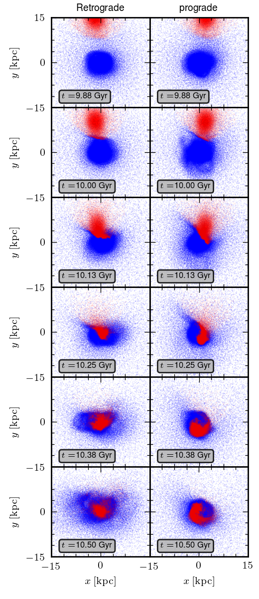
Figure 1: Gaseous infall on a dwarf galaxy. Black points (red in the online colour version) show the gas cloud falling in, gray points (blue in the online colour version) represent the gas of the dwarf galaxy. The left panels show the set-up of B3: a gas cloud falling in on a dwarf galaxy along a retrograde trajectory. The right panel shows the same set-up, but with the initial position of the gas cloud at $(2,30,0)$, resulting in a prograde trajectory.

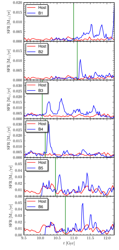
Figure 2: Star formation rate of bursting galaxies (black, blue in the online colour version), compared to that of their host galaxy in isolation (gray, red in the online colour version). The models are the ones from Table 1. Vertical lines roughly indicate when the gas cloud falls in on the dwarf galaxy.

Gaseous infall can trigger enhanced star formation in a galaxy in several ways. This can be seen from Figure 2, where we show the star formation rate in function of time of our six models (black, blue in the online colour version), compared to that of their host galaxies in isolation (gray, red in the online colour version). The vertical lines roughly show the moments the gas cloud enters the system.

When a very extended gas cloud is falling in on a slowly or non-rotating host galaxy, it can compress the gas of the host out of which stars will be born (B5). However, this will not necessarily happen and we might not find a starburst initially. However, all the gas of the host galaxy will be affected, making it more turbulent and more likely to collapse, resulting in a strong burst at later times (B1).

In the case of a rotating galaxy (B3), the story is mainly the same, except that the direction the gas cloud is falling in from is important as it was concluded in §3.1. In a retrograde merger, the two gas reservoirs collide and lots of gas is driven towards the galaxy center. This is clearly in the left column of Figure 1. In a prograde merger, the velocities of the two gas reservoirs closely match and the infalling gas cloud swirls around the galaxy center. There is no significant angular momentum exchange between both gas reservoirs, no gas is driven towards the galaxy center, and no starburst is ignited. Movies of this can be found online.

For the high-mass models, these results remain valid, but since we use a gas cloud of the same mass as in the low mass models, the gas of the galaxy will be less disturbed in this case.

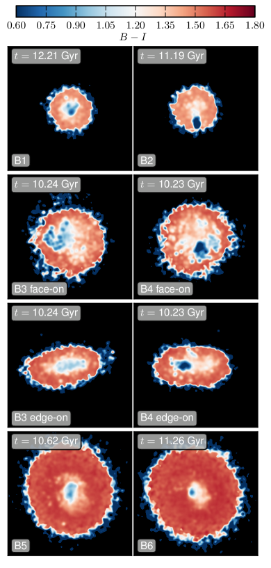
Figure 3: $B-I$ colour maps of our models during their bursts. All figures show 10 kpc in both directions.

On the other hand, when we use a compact gas cloud, the gas cloud will only have an effect very locally. When stars are being formed as a direct consequence of the gas cloud impact, they will be formed along the path of the gas cloud. This is the case in B2 and B4. In the absence of rotation, the host galaxy will not be able to efficiently stop the gas cloud, so star forming region will have an elongated shape. Rotating galaxies will be able to stop it more efficiently, resulting in a more centralized star forming region.

In B6, the CGC did not immediately trigger an increased star formation rate. Rather, most of the gas flew through the galaxy, since the gas cloud has been significantly accelerated by the high mass dwarf galaxy. Shortly after however, the gas falls back, triggering the burst. The starburst is more centralized compared to B2 and B4 since the gas falling back in now has low densities. Thus the stars will be formed out of the old gas of the galaxy, much like the simulations with EGCs.

Figure 3 shows $B-I$ colour images of our models, illustrating these effects. These images were obtained by setting up Cartesian luminosity grids in both bands, to which we applied a Gaussian filter (with $\sigma=100$ pc) to produce smoother images. The surface brightness of grid cells fainter than 29 mag/arcsec² were put to this magnitude. The blue edges are an artefact of this truncation, since the B-band will be rounded off more quickly than the I-band, so $B-I$ is underestimated.

3.3 Duration and periodicity of the starburst

After the initial burst, feedback in the form of SNII and stellar winds will efficiently remove the central gas reservoir and shut down the burst. Our bursts have lifetimes of a couple of 100 Myr, with a trend of stronger bursts having shorter lifetimes since the feedback will be more intense and remove the gas more efficiently. Indeed, in simulation B1 (top panel of Figure 2) we can identify a period of high star formation lasting $\sim 1$ Gyr, shortly followed by a strong but short burst.

After the burst, we have little gas in the centre of the galaxy, making it easy for the gas to fall back in and produce secondary bursts. We find these subsequent bursts in simulations B1, B3, B5 and B6, as can be seen in Figure 2.

3.4 Strength of the burst

The mass of the gas cloud plays an important role in the strength of the burst. The more massive it is, the stronger the burst it can trigger. A gas cloud with $M=5\cdot 10^{7}\,\mathrm{M}_{\odot}$ can temporarily increase the SFR with a factor 20 in the low mass dwarf galaxy models.

For gas clouds of the same mass, the increase in SFR will be less significant in more massive dwarfs. These dwarf galaxies are already forming stars at higher rates because of the higher gas content and deeper gravitational potential, making it harder to get a relative increase in SFR similar to that in the less massive dwarf galaxy models. The more massive dwarfs will still have an increased SFR during the burst.

The peak in SFR of each model and the burstfactor $b$, which is the relative increase compared to the average SFR of the host over the last 3 Gyr, are given in column 11 and 12 in Table 1.

Secondary bursts can be stronger than the initial burst (e.g. B1) but generally, we can expect the strength of each subsequent burst to be lower than the previous one.

3.5 Metallicity

It is to be expected that the metallicity of the dwarf galaxy will drop when we let a metal-poor gas cloud merge with it. In all our models, we found that the metallicity of the gas within 5 kpc of the dwarf galaxy centre indeed drops significantly when the gas cloud enters the system. We show the evolution of the gaseous metallicity in the top panels of Figure 4 and Figure 5 for B1 and B4, respectively.

However, looking at the B-band luminosity weighted metallicity of the stars (middle panel of Figure 4), we see that the metallicity can increase significantly following the merger. In fact, the only ones of the models discussed here where the metallicity drops are model B2 and B4, as can be seen in Figure 5 for the latter.

In the other models, the gas falling in will not reach high enough densities to form stars at initial impact so if there is an immediate starburst (e.g. B5), the stars will be formed out of the old, metal enriched gas. In the case of bursts arising from the disturbed gas (e.g. B1), the gas will be well mixed and stars will be formed out of metal enriched gas as well. In B2 and B4, on the contrary, a significant part of the starburst is consuming the new, metal-poor gas.

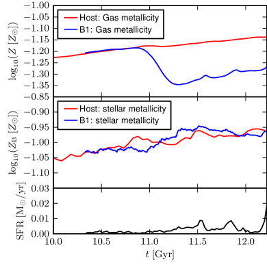
Figure 4: Evolution of the metallicity of the gas within 5 kpc (top panel), the B-band luminosity weighted metallicity of the stars (middle panel) and the SFR (bottom panel) of simulation B1. Gray (red in the online colour version) shows the model in isolation, black (blue in the online colour version) shows what happens when a gas cloud falls in.

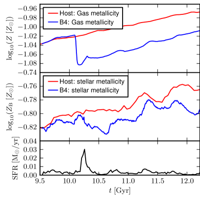
Figure 5: Same as Figure 4 but now for simulation B4.

3.6 Colour

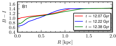
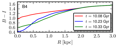
Figure 6: $B-I$ colour profile of model B1 (top) and B4 (bottom) before (light gray, red in the online colour version), during (black, blue in the online colour version) and after (gray, green in the online colour version) their respective bursts.

Given the presence of irregular star formation knots in our galaxies during the starburst, we obtain colour profiles using a technique similar to isophotal integration for obtaining surface brightness profiles (Papaderos et al., 1996; Micheva et al., 2013a; Micheva et al., 2013b). We start from the Cartesian grids used to produce the $B-I$ colourmaps in Figure 3. For each colour value, we determine the number of grid cells with colours bluer than this value and add their areas together. These areas are then converted to the equivalent radius of a circle with the same area. This method gives the radius in function of colour and it will produce a monotonically rising profile. The employed technique comes with the caveat that at some point, grid cells containing no stellar particles start influencing the profile. We cut off our profile before this happens. Also, the obtained radius can not be interpreted as a physical distance from the centre of the galaxy, unless in regular circular or elliptical systems.

The result for B1 and B4 can be seen in Figure 6, in which the colour profiles before (light gray, red in the online colour version), during (black, blue in the online colour version) and after (gray, green in the online colour version) their respective bursts are shown. We note that B1 has a strong burst right at the end of the simulation (top panel of Figure 2). To investigate what happens after the burst, we continued this simulation until $t=12.7$ Gyr. For this simulation, we see a clear drop in colour for $R\lesssim 1$ kpc during the burst, with colour difference of over 0.3 mag in the centre, compared to before the burst. After the burst, the galaxy has become redder in the centre than during the burst, but is still bluer than before the burst. For $R\gtrsim 0.5$ kpc, the post-burst galaxy is bluer than during the burst. This can be due to recently formed stars moving to higher radii or stars being formed by the intense feedback following the central starburst. Since the stars are being formed from the metal-enriched gas of the dwarf galaxy, the bluer colours can be solely attributed by the age of the stellar population. For B4, the trend is the same, but we find much bluer colours: $B-I$ drops by $\sim 0.6$ mag in the centre, compared to before the burst. The reason is that now the stars are being formed from the metal-poor gas of the gas cloud.

3.7 Density profiles

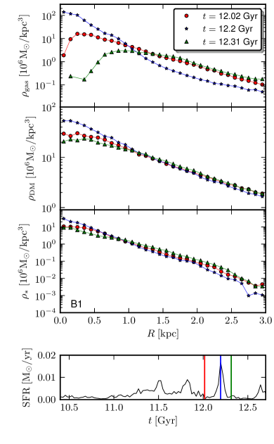
Figure 7: Gas, dark matter and stellar density profile of B1 before (light gray circles, red in the online colour version), during (black stars, blue in the online colour version) and after the starburst event (gray triangles, green in the online colour version).

Figure 7 shows the density profile of the gas, dark matter and stars, at times before (light gray circles, red in the online colour version), during (black stars, blue in the online colour version) and after the burst (gray triangles, green in the online colour version). We see that for all the components, the central density rises significantly during the burst compared to before, while the density at higher radii drops. After the burst, the central density drops, even below the density before the burst, and gets higher in the outer regions. This effect is strongest for the gas.

No matter how the starburst is triggered exactly, the reason we have a burst is because the gas reaches a high density in a certain area. So the higher central gaseous densities should not come as a surprise. However, this large central gaseous mass causes the rest of the galaxy to contract. Hence we get a more compact galaxy, with a higher concentration of gas, dark matter and stars in the centre (also because of the high star formation) and a lower concentration in the outskirts of the galaxy. This redistribution of matter can in other words be attributed to the deepening of the gravitational potential. This process occurs in all models, albeit less significant in B2 and B4, where the impact of the CGC is a more local effect.

Shortly after the burst, the gas will receive a lot of feedback from the young stellar particles and will be blown to larger radii. The gravitational potential becomes shallower and the dark matter and stars also move outwards, resulting in a more diffuse galaxy. This process is present in all models and should be only dependent on the strength of the burst, as this determines the amount of feedback and thus the efficiency of the removal of the gas.

Since the expansion due to feedback will be faster than the previous collapse to the centre, the former will have a larger effect. So we are possibly left with a postburst galaxy that is more diffuse than preburst.

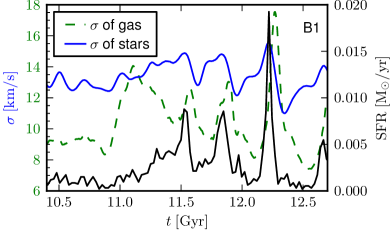
Figure 8: Velocity dispersion of the gas (gray dashed line, green in the online colour version) and of the stars (light gray solid line, blue in the online colour version) compared to the SFR (black solid line) for simulation B1.

3.8 Velocity dispersion

We have a look at the velocity dispersion of both the gas (within 5 kpc) and the stars, defined as

$$\sigma=\sqrt{\frac{\sigma_{x}^{2}+\sigma_{y}^{2}+\sigma_{z}^{2}}{3}}.$$ (12)

In Figure 8, we show the evolution of $\sigma$ of the gas and of the stars of B1, along with the SFR. When the gas enters the system (at $\sim$ 11 Gyr), the velocity dispersion of the gas increases significantely. After it drops back, it follows the general trend of the SFR with a slight delay. The velocity dispersion of the stars increases and decreases together with the SFR. This trend is present in all our models, albeit less significant in the more massive ones B5 and B6.

Before the gas can form stars, it has to cool down and collapse, thus lowering its velocity dispersion. As new stars are being formed, gas with low $\sigma$ is removed and, more importantly, the surrounding gas gets heated and it expands, increasing the gaseous velocity dispersion. This explains why the velocity dispersion of the gas follows the star formation rate with a slight delay.

On the other hand, as the gas collapses and produces a burst, the stellar body also becomes more compact and the velocity dispersion of the stars increases during a starburst.

Shortly after the burst, the stellar body is more diffuse and the velocity dispersion drops. This explains the concurrence of the stellar velocity dispersion curve and the SFR in Figure 8. The same is true for the dark matter. As an extra effect, we have a lot of young stars with low $\sigma$, further decreasing the velocity dispersion of the stars.

3.9 Isophotal maps

Figure 9 shows the isophotal maps of our models during their strongest peak in star formation. To obtain these, we produced a cartesian grid (with cells of width 70 pc), calculated the surface brightness in each cell, applied a Gaussian filter ($\sigma=100$ pc) to smooth the data and plotted the contours. Isophotes go from $\mu=$ 27 mag/arcsec² (most outer and faintest, reddest in the online colour version) up to $\mu=$ 21.5 mag/arcsec² (most inner and darkest, bluest in the online colour version), in increments of 0.5 mag/arcsec²

Model B1 has a regular, slightly off-centre star forming region and the outer isophotes are nicely elliptical. Model B2 has a very off-centre star forming region, giving the entire galaxy a very elongated shape.

For B3 and B4, the models with a host with strong rotation, we show both a face-on and edge-on view. Face-on, both have very irregular outer isophotes, which can be explained by the rotation (Schroyen et al., 2011). The star forming region in both models is very off-centre. In B3, it is very irregular, while the star forming region in B4 is more regular. However, due to it being off-centre, it also gives the galaxy an elongated shape.

Edge-on, the outer isophotes are flattened and more regular. In B3, the star forming region is off-centre and slightly irregular, while in B4, it is very centralized.

Both the high mass models B5 and B6 show a regular, slightly off-centre star forming region embedded in an elliptical host galaxy.

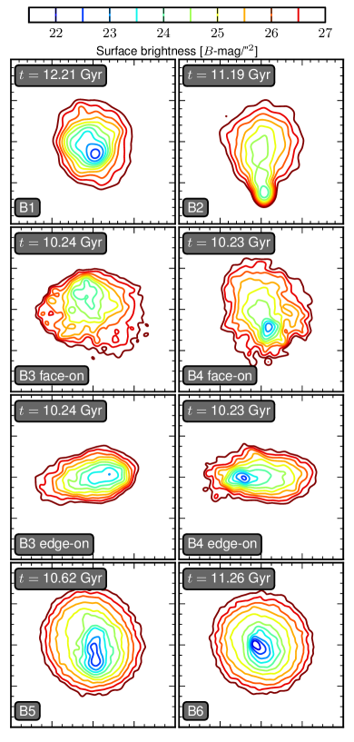
Figure 9: Isophotal maps in the B-band of our models during their burst. Sides for B1 and B2 are 4 kpc on both sides, for B3 and B4 6 kpc and for B5 and B6 both sides are 7 kpc. For B3 and B4, the models with a strongly rotating host galaxy, both the edge-on as the face-on maps are shown. Isophotes go from $\mu=$ 27 mag/arcsec² (most outer and faintest, reddest in the online colour version) up to $\mu=$ 21.5 mag/arcsec² (most inner and darkest, bluest in the online colour version), in increments of 0.5 mag/arcsec²

4 Discussion

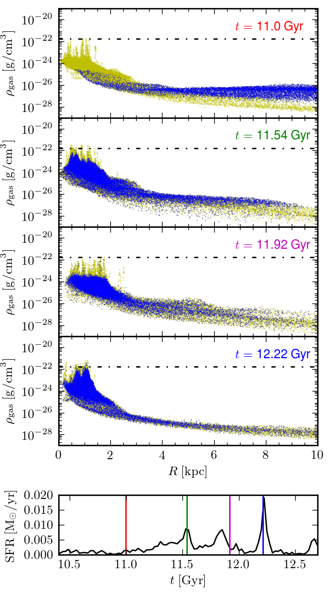
Figure 10: Scatter plot of the density and radius of all gas particles of simulation B1. Black points (yellow in the online colour version) represent the old gas of the dwarf galaxy, gray points (blue in the online colour version) show the infalling gas cloud. The dash-dot line shows the density threshold for star formation.

4.1 The triggering mechanism

Having established that an infalling gas cloud can trigger a significant increase in the star formation of a dwarf galaxy, we can wonder what exactly is the reason of this increase. In Figure 10, we show the radius and density of all gas particles in simulation B1 at different times. The gas already present in the dwarf galaxy is shown by black dots (yellow in the online colour version), while the gray dots (blue in the online colour version) represent the newly added gas of the gas cloud. The first panel ($t=11$ Gyr) shows the extended gas cloud falling in. In the second panel ($t=11.54$ Gyr), the influx of gas has led to the formation of many star-forming clouds and consequently to an increased SFR. Remarkably, virtually no “new” gas particles are mixed into these high-density, star-forming regions and the stars are being formed out of the “old” gas of the galaxy. This causes the stellar metallicity to further increase (§3.5). Clearly, this first sharp increase of the SFR is the direct result of the gas cloud compressing the old gas of the galaxy. This initial increase in SFR when the gas cloud enters the system, can be seen in all our models, except in B6. On the other hand, when the gas cloud is initially dense enough, stars can form out of the new gas, resulting in a more metal-poor starburst. This occurs in simulations B2 and B4.

Moreover, we can conclude from our simulations that gas cloud mergers also have a longer lasting impact on the SFR. The increased turbulence of the interstellar gas following a merger and starburst lasts for several Gyrs, as can be seen in the velocity disperion of the gas (§3.8). During this time, the gas appears to be much more prone to gravitational collapse and therefore to subsequent starburst events. In the third panel ($t=11.92$ Gyr) of Figure 10, the feedback following the previous star formation has blown out the gas from the central region, lowering the SFR. Around $R\sim 5$ kpc, for instance, one can see this gas being blown out. In the fourth panel ($t=12.22$ Gyr), the gas has fallen back in and a starburst ensues, over a gigayear after the merger. Now, the gas is well mixed and the stars are being formed out of both the old and the newly added gas.

4.2 Surface brightness profile

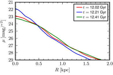
Figure 11: Isophotal surface brightness profile in the B-band before (light gray, red in the online colour version), during (black, blue in the online colour version) and after (dark gray, green in the online colour version) the starburst in simulation B1.

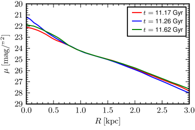
Figure 12: Same as Figure 11 but for simulation B6.

As shown in §3.7, the stellar body of the galaxy becomes more compact during a starburst, in agreement with e.g. Papaderos et al. (1996); Micheva et al. (2013a); Micheva et al. (2013b). They draw their conclusions by investigating the surface brightness profiles, usually obtained using isophotal integration due to the possible irregular shapes of BCDs. This method was already used to produce the colour profiles in §3.6, and now we obtain surface brightness profiles in a similar way. Figures 11 and 12 show the B-band surface brightness (SB) for model B1 and B6 respectively, before (light gray, red in the online colour version), during (black, blue in the online colour version) and after (dark gray, green in the online colour version) the starburst

For the strong burst in B1 at $t\approx 12.2$ Gyr, we find an increase in SB in the centre, by about 1 mag/arcsec², due to the bright, newly formed stellar populations. Moreover, as shown in §3.7, the outer stars are moving inwards causing the SB outside the inner $\sim 0.5$ kpc to decrease. This results in a overall steeper surface brightness profile. For the more massive model B6, we also find an increased SB in the centre and a decreased SB at large radii, albeit less pronounced than in the low mass model B1. This is because the burst is weaker relative to the average SFR of the host galaxy (see Table 1).

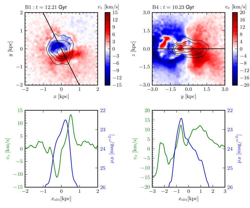
Figure 13: Top: velocity field of the gas overlaid with the surface brightness contours in the B-band (top). Bottom: the line-of-sight velocity (gray, green in the online colour version) and the surface brightness (black, blue in the online colour version) along a slit put on the major axis for simulations B1 (left) and B4 (right).

4.3 Subtypes

Based on the isophotal maps discussed in §3.9, we can classify our models according to the classification scheme of Loose & Thuan (1986). Since our bursting models clearly have an old stellar population and we do not let two dwarf galaxies merge, we do not expect i0 or iI,M BCDs to be found in our simulations.

B1 and B6 have regular isophotes and a nuclear, albeit slightly off-centre, starburst and could thus be classified as nE BCDs. B5 has regular isophotes as well but the starburst is very off-centre and/or irregular, so we classify this model as a iE BCD. When viewing B3 and B4 face-on, we see an irregular, off-centre starburst in a highly irregular host. One would classify these as iI BCDs. However, when B3 and B4 are viewed edge-on, the starburst region can be significantly off-centre, giving these models a flattened, cometary look. For this viewing geometry, B3 and B4 would be classified as a iI,C. The same classification applies to B2.

Based on these findings and the qualitative differences between the models, we can propose an explanation and make predictions for the different subtypes and their properties:

• iE BCDs can be produced when the infalling gas cloud immediately triggers a burst in a not, or only slowly, rotating dwarf, as the dense gas will most likely not be centralized and have irregular shapes and the outer isophotes will have regular shapes (e.g. models B2, B5). Of course, if the star-forming region is significantly off-centre, the galaxy might be labelled as a cometary BCD.

• nE BCDs on the other hand will more likely be found in secondary bursts in the same host galaxy (e.g. models B1, B6) as gas has re-accumulated at the galaxy centre and ignited in a new starburst. However, the supernova feedback from this central starburst can lead to star formation in dense clouds on the edges of supernova blown bubbles, resulting in more irregular star forming regions. Thus, a nE BCD may evolve into an iE BCD.

• iI BCDs are found in rotating host galaxies (e.g. models B3, B4). Schroyen et al. (2011) found that in simulated dwarf galaxies with a significant amount of rotation, star formation occurs continuously over the galactic body, in contrast to a more bursty, centralized star formation in dwarfs with slow (or no) rotation. This more dispersed star formation results in an irregular stellar body. So when the galaxy enters the starburst phase, the star forming region will most likely be off-centre and have an irregular shape. When looking at an iI BCD with off-centre star formation, it could be classified as an iI,C BCD, when viewed edge-on.

Our other simulations which produced a burst but which were not explicitly discussed in this paper, all agree with this explanation for the classification of the different subtypes as well.

There are indeed a number of observations that support this picture. iI BCDs were found to be in general bluer (Gil de Paz et al., 2003), more gas-rich, and more metal-poor (Zhao et al., 2013) than nE/iE BCDs and their HI distribution is more clumpy rather than centralized (Taylor et al., 1994; van Zee et al., 1998; Thuan et al., 2004). All of these findings can be explained by the degree of rotation they have (Schroyen et al., 2011). Thuan et al. (2004) found that the nE and iE BCDs in their sample show no regular rotation, while the two cometary BCDs in their sample are rotationally dominated. At least 5 of the 7 iI,C BCDs investigated in Sánchez Almeida et al. (2013) are rotating. Observations have shown that some iE BCDs have their star forming regions organized in a ring (Gil de Paz et al., 2003), supporting the idea of propagating star formaton and an evolution from nE to iE BCD.

Noeske et al. (2000) found that the host galaxies of iI,C BCDs generally have structural parameters that lie between those of BCDs and other dwarfs. If our models are indicative for real life BCDs, the fact that these are less compact than nE/iE BCDs can be explained in two ways. Firstly, if star formation occurs very off-centre, there will not be such a large increase in the central mass and thus the gravitational potential will deepen less. This results in a less compacthost galaxy. Secondly, iI,C BCDs are likely to be found in rotating host galaxies, which are generally already more diffuse. On the other hand, when looking at a flattened galaxy edge-on, the surface brightness will drop more rapidly, resulting in a seemingly more compact galaxy, as opposed to when we would view it face-on. We thus propose that iI BCDs should be even more diffuse than iI,C BCDs, and their hosts will have scale lengths and central surface brightnesses in the parameter space occupied by dE and dIs. To the best of our knowledge, no large sample study has been performed of the structural parameters of the host of iI BCDs. The sample of Micheva et al. (2013a); Micheva et al. (2013b) contains some iI BCDs, who do indeed tend to lie in the parameter region of the dEs and dIs.

4.4 Gas kinematics

As the gas and stellar component of the galaxy becomes more centralized, we expect that their rotational velocity will increase due to conservation of angular momentum. This would explain the observations by van Zee et al. (2001), who found that the HI of BCDs have steeply rising rotation curves. Figure 13 shows the 2-dimensional gaseous line-of-sight velocity fields of B1 and B4 (edge-on view), left and right respectively, during the burst, overlaid with the B-luminosity contours. We show these two quantities along a slit placed along the major axis to mimic how this would be detected observationally. For B1, we indeed find a steeply rising rotation curve.

For B4, we see that the galaxy overall has solid body rotation around the minor axis (the $z$-axis), but the kinematics of the starburst region are very different (as found by e.g. Östlin et al., 2004; Koleva et al., 2014). In this model, a CGC has fallen in, coming from the right side in Figure 13. This impact will cause a significant amount of gas in the white (red in the online colour version) region (with positive $v_{x}$) to move to the black (blue in the online colour version) region (with negative $v_{x}$), causing a disturbance in the solid body rotation pattern of the galaxy. Looking along the $y$-axis (along which the gas cloud fell in), we will see a similar disturbance while in the $z$-axis, no significant difference will be found.

We can conclude that if the burst happens right after the gas cloud fell in and depending on our viewing angle at the galaxy, the gas can have very disturbed kinematics. In secondary bursts on the other hand, like in B1, the gas will most likely show no disturbance.

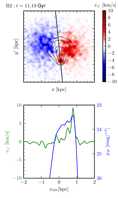
Figure 14: Same as in Figure 13 but for the stars of simulation B2. Note that the simulation was rotated $\sim 50^{\circ}$ around the $x$-axis to show the effects more clearly.

4.5 Stellar kinematics

Koleva et al. (2014) found that the star forming regions of BCDs can have kinematics that are very different from those of their host galaxies. The top panel of Figure 14 shows the velocity fields of the stars of simulation B2. The radial velocity and surface brightness along a slit along the major axis is shown in the bottom panel. As we can see, the velocity of the gas cloud that fell in results in a star forming region with different kinematical properties than that of the host galaxy. Thus, our simulations are able to reproduce the findings of Koleva et al. (2014), at least for simulations with a compact infalling gas cloud, as in B2.

4.6 Evolutionary path

It has been long discussed what BCDs will look like when their starburst has faded. Among others, Papaderos et al. (1996) suggested that postburst dwarf galaxies can not reside in the general dE or dI population without a drastic change in their structural parameters. van Zee et al. (2001) state that a passive evolution to dE is unlikely as it would require a significant loss of angular momentum. They suggest that so-called compact dI (e.g. van Zee, 2000; Patterson & Thuan, 1996) are candidate faded BCDs, since they have similar scale lengths and have significant colour gradients.

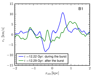
Figure 15: Line of sight velocity of the gas along the same slit as in Figure 13 for simulation B1 during (black line, or blue in the online colour version) and after (gray line, or green in the online colour version) the starburst.

Looking at our models, we find that generally postburst galaxies tend to be more diffuse after the burst than during the burst, when the galaxy would be classified as a BCD. Often, the galaxy is even more diffuse than before the burst(s), placing it within the structural parameter space occupied by dEs and dIs. Moreover, as the galaxy re-expands after the burst, the steep rise of its rotation curve disappears (as can be seen in Figure 15), removing also this obstacle to a possible BCD-dI transition. On top of that, the time-scale of a burst is much smaller than the gas exhaustion time and the feedback following the starburst is not strong enough to completely remove all the gas of the galaxy. Thus BCDs that were dIs before the burst will be dIs again after the burst.

4.7 The role of feedback

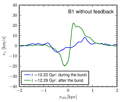
Figure 16: Same as in Figure 15, but for a model with both star formation and feedback turned off after the burst. Note that the vertical scale here is different from that of Figure 15.

Stellar feedback through supernovae and stellar winds is assumed to play a vital role in quenching the starburst. Furthermore, it seems that the strong feedback effects result in a diffuse post-burst galaxy, with shallow rotation curves and low stellar velocity dispersion, as discussed in paragraphs 3.7, 4.6 and 3.8. To confirm that this evolution is primarily due to feedback, we have rerun simulation B1, but with feedback turned off after $t=12.22$ Gyr (the time of the burst). Since there would be no way of quenching the starburst, we also turn off star formation.

There is now nothing to prevent the gas from collapsing further, resulting in a very deep gravitational potential, a very compact galaxy (in both gas, stars and dark matter), high velocity dispersion and a very steep rotation curve. The latter is shown in Figure 16.

5 Summary

We have run a large suite of numerical simulations of gas clouds falling in on dwarf galaxies, using different galaxy and cloud masses and sizes, and different orbital parameters. Our goal was to test whether starbursts could be ignited this way and whether the resulting galaxies could explain some of the properties of observed Blue Compact Dwarfs.

Based on our simulations, we conclude that infalling gas can indeed trigger a starburst in dwarf galaxies by significantly disturbing the gas, especially in dwarf galaxies with $M_{B}\gtrsim-14$ mag. We found that gas cloud masses significantly below $\sim 10^{7}$ M_⊙ do not trigger starbursts in the mass regime of the dwarfs simulated by us. If such clouds are rare, then this tells us that, although this is a viable way of triggering starbursts in dwarfs, this is not the triggering mechanism in the majority of the BCDs. Of course, less massive clouds could still trigger starbursts in dwarf galaxies with lower masses than the ones we simulated. The starburst phase seems to be episodic, alternated with periods of little star formation. Following the infall of metal-poor gas, the overall gas metallicity of the galaxy drops. However, the stellar metallicity can either increase or decrease, depending on the source of the gas from which the stars are formed: the pre-enriched galaxy or the metal-poor infalling gas cloud. In most of our models, the stars were formed from the old gas, resulting in metal-rich stars. Only in models with compact infalling gas clouds can stars form from the newly arrived gas, leading to more metal-poor newborn stars. Following the impact of the gas cloud, the gas kinematics can become very disturbed. Stars that form from kinematically distinct gas clumps tend to be also kinematically peculiar when compared with the stellar body of the galaxy.

As gas flows towards the galaxy centre to fuel the central starburst, the gravitational potential deepens. In response, the whole body of the galaxy becomes more compact and the rotation curve steepens. Once gas is rapidly evacuated from the galaxy centre by supernova feedback, the galaxy re-expands and becomes more diffuse again, flattening the rotation curve. This removes some of the arguments against evolutionary links between BCDs and dIs.

As discussed in paragraph 4.3, we can attempt an explanation for the physical differences between the subtypes of BCDs in the classification scheme of Loose & Thuan (1986) within the scope of our simulations:

• nE and iE BCDs have host galaxies that are slowly (or not) rotating. nE BCDs can evolve into iE types as star formation propagates through the host galaxy.

• iI BCDs have flattened host galaxies with strong rotation, viewed approximately face-on.

• iI,C BCDs have flattened, strongly rotating host galaxy, viewed approximately edge-on.

References

- Bekki (2008) Bekki K., 2008, MNRAS, 388, L10
- Brinks (1990) Brinks E., 1990, II Zwicky 33: star formation induced by a recent interaction.. pp 146–149
- Brinks & Klein (1988) Brinks E., Klein U., 1988, MNRAS, 231, 63P
- Cairós et al. (2001) Cairós L. M., Vílchez J. M., González Pérez J. N., Iglesias-Páramo J., Caon N., 2001, ApJS, 133, 321
- Campos-Aguilar & Moles (1991) Campos-Aguilar A., Moles M., 1991, A&A, 241, 358
- Campos-Aguilar et al. (1993) Campos-Aguilar A., Moles M., Masegosa J., 1993, AJ, 106, 1784
- Cloet-Osselaer et al. (2012) Cloet-Osselaer A., De Rijcke S., Schroyen J., Dury V., 2012, MNRAS, 423, 735
- Cloet-Osselaer et al. (2014) Cloet-Osselaer A., De Rijcke S., Vandenbroucke B., Schroyen J., Koleva M., Verbeke R., 2014, Numerical simulations of dwarf galaxy merger trees, Submitted to MNRAS
- De Rijcke et al. (2013) De Rijcke S., Schroyen J., Vandenbroucke B., Jachowicz N., Decroos J., Cloet-Osselaer A., Koleva M., 2013, MNRAS, 433, 3005
- Di Matteo et al. (2007) Di Matteo P., Combes F., Melchior A.-L., Semelin B., 2007, A&A, 468, 61
- Elmegreen et al. (2012) Elmegreen B. G., Zhang H.-X., Hunter D. A., 2012, ApJ, 747, 105
- Gil de Paz et al. (2003) Gil de Paz A., Madore B. F., Pevunova O., 2003, ApJS, 147, 29
- Gordon & Gottesman (1981) Gordon D., Gottesman S. T., 1981, AJ, 86, 161
- Governato et al. (2010) Governato F., Brook C., Mayer L., Brooks A., Rhee G., Wadsley J., Jonsson P., Willman B., Stinson G., Quinn T., Madau P., 2010, Nature, 463, 203
- Hoffman et al. (2003) Hoffman G. L., Brosch N., Salpeter E. E., Carle N. J., 2003, AJ, 126, 2774
- Hunter & Hoffman (1999) Hunter D. A., Hoffman L., 1999, AJ, 117, 2789
- Izotov & Thuan (1999) Izotov Y. I., Thuan T. X., 1999, ApJ, 511, 639
- Izotov et al. (1994) Izotov Y. I., Thuan T. X., Lipovetsky V. A., 1994, ApJ, 435, 647
- Kereš & Hernquist (2009) Kereš D., Hernquist L., 2009, ApJL, 700, L1
- Koleva et al. (2014) Koleva M., De Rijcke S., Zeilinger W. W., Verbeke R., Schroyen J., Vermeylen L., 2014, MNRAS, 441, 452
- Kunth et al. (1988) Kunth D., Maurogordato S., Vigroux L., 1988, A&A, 204, 10
- Lehner et al. (2009) Lehner N., Staveley-Smith L., Howk J. C., 2009, ApJ, 702, 940
- Lelli et al. (2014) Lelli F., Verheijen M., Fraternali F., 2014, ArXiv e-prints
- Lelli et al. (2012a) Lelli F., Verheijen M., Fraternali F., Sancisi R., 2012a, A&A, 537, A72
- Lelli et al. (2012b) Lelli F., Verheijen M., Fraternali F., Sancisi R., 2012b, A&A, 544, A145
- Loose & Thuan (1986) Loose H.-H., Thuan T. X., 1986, in Kunth D., Thuan T. X., Tran Thanh Van J., Lequeux J., Audouze J., eds, Star-forming Dwarf Galaxies and Related Objects The morphology and structure of blue compact dwarf galaxies from CCD observations.. pp 73–88
- López-Sánchez et al. (2012) López-Sánchez Á. R., Koribalski B. S., van Eymeren J., Esteban C., Kirby E., Jerjen H., Lonsdale N., 2012, MNRAS, 419, 1051
- Micheva et al. (2013a) Micheva G., Östlin G., Bergvall N., Zackrisson E., Masegosa J., Marquez I., Marquart T., Durret F., 2013, MNRAS, 431, 102
- Micheva et al. (2013b) Micheva G., Östlin G., Zackrisson E., Bergvall N., Marquart T., Masegosa J., Marquez I., Cumming R. J., Durret F., 2013, A&A, 556, A10
- Navarro et al. (1996) Navarro J. F., Frenk C. S., White S. D. M., 1996, ApJ, 462, 563
- Noeske et al. (2000) Noeske K. G., Guseva N. G., Fricke K. J., Izotov Y. I., Papaderos P., Thuan T. X., 2000, A&A, 361, 33
- Noeske et al. (2001) Noeske K. G., Iglesias-Páramo J., Vílchez J. M., Papaderos P., Fricke K. J., 2001, A&A, 371, 806
- Oosterloo et al. (2007) Oosterloo T., Fraternali F., Sancisi R., 2007, AJ, 134, 1019
- Östlin et al. (2001) Östlin G., Amram P., Bergvall N., Masegosa J., Boulesteix J., Márquez I., 2001, A&A, 374, 800
- Östlin et al. (2004) Östlin G., Cumming R. J., Amram P., Bergvall N., Kunth D., Márquez I., Masegosa J., Zackrisson E., 2004, A&A, 419, L43
- Papaderos et al. (1996) Papaderos P., Loose H.-H., Fricke K. J., Thuan T. X., 1996, A&A, 314, 59
- Papaderos et al. (1996) Papaderos P., Loose H.-H., Thuan T. X., Fricke K. J., 1996, A&AS, 120, 207
- Patterson & Thuan (1996) Patterson R. J., Thuan T. X., 1996, ApJS, 107, 103
- Pisano et al. (2007) Pisano D. J., Barnes D. G., Gibson B. K., Staveley-Smith L., Freeman K. C., Kilborn V. A., 2007, ApJ, 662, 959
- Putman et al. (2009) Putman M. E., Peek J. E. G., Muratov A., Gnedin O. Y., Hsu W., Douglas K. A., Heiles C., Stanimirovic S., Korpela E. J., Gibson S. J., 2009, ApJ, 703, 1486
- Ramya et al. (2009) Ramya S., Kantharia N. G., Prabhu T. P., 2009, in Saikia D. J., Green D. A., Gupta Y., Venturi T., eds, The Low-Frequency Radio Universe Vol. 407 of Astronomical Society of the Pacific Conference Series, A Radio Continuum and H I Study of Optically Selected Blue Compact Dwarf Galaxies: Mrk 1039 and Mrk 0104. p. 114
- Read & Gilmore (2005) Read J. I., Gilmore G., 2005, MNRAS, 356, 107
- Revaz et al. (2009) Revaz Y., Jablonka P., Sawala T., Hill V., Letarte B., Irwin M., Battaglia G., Helmi A., Shetrone M. D., Tolstoy E., Venn K. A., 2009, A&A, 501, 189
- Salpeter (1955) Salpeter E. E., 1955, ApJ, 121, 161
- Salzer & Norton (1999) Salzer J. J., Norton S. A., 1999, in Davies J. I., Impey C., Phillips S., eds, The Low Surface Brightness Universe Vol. 170 of Astronomical Society of the Pacific Conference Series, Gas rich Low Surface Brightness galaxies - progenitors of blue compact dwarfs?. p. 253
- Sánchez Almeida et al. (2014) Sánchez Almeida J., Morales-Luis A. B., Muñoz-Tuñón C., Elmegreen D. M., Elmegreen B. G., Méndez-Abreu J., 2014, ApJ, 783, 45
- Sánchez Almeida et al. (2013) Sánchez Almeida J., Muñoz-Tuñón C., Elmegreen D. M., Elmegreen B. G., Méndez-Abreu J., 2013, ApJ, 767, 74
- Schmidt (1959) Schmidt M., 1959, ApJ, 129, 243
- Schroyen et al. (2013) Schroyen J., De Rijcke S., Koleva M., Cloet-Osselaer A., Vandenbroucke B., 2013, MNRAS, 434, 888
- Schroyen et al. (2011) Schroyen J., De Rijcke S., Valcke S., Cloet-Osselaer A., Dejonghe H., 2011, MNRAS
- Simpson & Gottesman (2000) Simpson C. E., Gottesman S. T., 2000, AJ, 120, 2975
- Simpson et al. (2011) Simpson C. E., Hunter D. A., Nordgren T. E., Brinks E., Elmegreen B. G., Ashley T., Lynds R., McIntyre V. J., O’Neil E. J., Östlin G., Westpfahl D. J., Wilcots E. M., 2011, AJ, 142, 82
- Springel (2005) Springel V., 2005, MNRAS, 364, 1105
- Stinson et al. (2007) Stinson G. S., Dalcanton J. J., Quinn T., Kaufmann T., Wadsley J., 2007, ApJ, 667, 170
- Taylor et al. (1995) Taylor C. L., Brinks E., Grashuis R. M., Skillman E. D., 1995, ApJS, 99, 427
- Taylor et al. (1994) Taylor C. L., Brinks E., Pogge R. W., Skillman E. D., 1994, AJ, 107, 971
- Telles & Terlevich (1995) Telles E., Terlevich R., 1995, MNRAS, 275, 1
- Terlevich et al. (1991) Terlevich R., Melnick J., Masegosa J., Moles M., Copetti M. V. F., 1991, A&AS, 91, 285
- Teyssier et al. (2013) Teyssier R., Pontzen A., Dubois Y., Read J. I., 2013, MNRAS, 429, 3068
- Thuan et al. (2004) Thuan T. X., Hibbard J. E., Lévrier F., 2004, AJ, 128, 617
- Thuan & Martin (1981) Thuan T. X., Martin G. E., 1981, ApJ, 247, 823
- Valcke et al. (2008) Valcke S., De Rijcke S., Dejonghe H., 2008, MNRAS, 389, 1111
- Valcke et al. (2010) Valcke S., De Rijcke S., Rödiger E., Dejonghe H., 2010, MNRAS, 408, 71
- van der Hulst & Sancisi (1988) van der Hulst T., Sancisi R., 1988, AJ, 95, 1354
- van Woerden & Wakker (2004) van Woerden H., Wakker B. P., 2004, in van Woerden H., Wakker B. P., Schwarz U. J., de Boer K. S., eds, High Velocity Clouds Vol. 312 of Astrophysics and Space Science Library, Distances and Metallicities of HVCS. p. 195
- van Zee (2000) van Zee L., 2000, AJ, 119, 2757
- van Zee et al. (2001) van Zee L., Salzer J. J., Skillman E. D., 2001, AJ, 122, 121
- van Zee et al. (1998) van Zee L., Skillman E. D., Salzer J. J., 1998, AJ, 116, 1186
- Yoshii et al. (1996) Yoshii Y., Tsujimoto T., Nomoto K., 1996, ApJ, 462, 266
- Zhao et al. (2013) Zhao Y., Gao Y., Gu Q., 2013, ApJ, 764, 44
- Zwicky (1964) Zwicky I. F., 1964, ApJ, 140, 1467