Leader-following Consensus of Multi-agent Systems over Finite Fields

Abstract

The leader-following consensus problem of multi-agent systems over finite fields ${\mathbb{F}}_{p}$ is considered in this paper. Dynamics of each agent is governed by a linear equation over ${\mathbb{F}}_{p}$, where a distributed control protocol is utilized by the followers. Sufficient and/or necessary conditions on system matrices and graph weights in ${\mathbb{F}}_{p}$ are provided for the followers to track the leader.

I Introduction

The distributed control of multi-agent systems have attracted intensive attentions these years. Various approaches are proposed to handle different problems for agents with different communication and dynamic constraints. In most existing literature, the states of agents and the information exchange between agents are defined as real numbers or quantized values [1],[9], [13],[18]. Recently, a finite field formalism was proposed to investigate multi-agent systems where the states of each agent are considered elements of a finite field [19],[24]. The states of each agent are updated iteratively as a weighted sum of the states of its neighbors, where the operations are performed as modular arithmetic in that field. Such a system is not only interesting theoretically but also has advantages such as smaller convergence time and resilience to communication noises, with applications to quantized control and distributed estimation.

Dynamical systems that take values from finite sets are ubiquitous. Consensus or synchronization of such systems were also widely investigated, such as quantized consensus, logical consensus, synchronization of finite automata [4],[7], [9],[28]. In fact, finite fields provide one convenient approach to model some of these systems. In the communication and circuits areas, linear systems over finite fields have long been studied[3], [11],[12]. In the control community, Kalman et al developed an algebraic theory for linear systems over an arbitrary field in the 1960s, by merging automata theory and module theory [8]. However, to the best of our knowledge, there are few results on the consensus/synchronization of linear multi-agent systems over finite fields, especially in a distributed manner. It is very interesting to consider how to achieve desired collective behaviors through local information for such systems. In [24], a first-principle approach was proposed to establish a graph-theoretic characterization of the controllability and observability problems for linear systems over finite fields. These results were applied to state placement and information dissemination of agents whose states are quantized values. In [19], some sufficient and necessary conditions on network weights and topology were given for the consensus of a group of agents on finite fields. It was shown that analyzing tools for real valued multi-agent systems cannot be applied straightforwardly to these systems in finite fields.

The objective of this paper is to study the leader-following consensus problem of multi-agent systems over finite fields. Dynamics of the leader and the followers are governed by linear equations in a given finite field. For the leader, the equation is autonomous; for each follower, it has local information input that is a weighted sum of relative states between itself and its neighbors, where the operations are done as modular arithmetic. We first formulate the leader-following consensus problem on finite fields. Then under some assumptions, we provide sufficient and/or necessary consensus conditions on system matrices and graph weights. Compared with existing results on multi-agent systems over finite fields [19],[24], agents considered here have higher order dynamics and the interaction graphs are directed acyclic and could possibly be time-varying.

The rest of the paper is organized as follows. In section 2, some preliminaries on finite fields and linear systems over finite fields are given. After the problem is formulated in section 3, our main results are provided in section 4, along with an illustrative example. In section 5 some conclusions are presented finally.

II Preliminaries

In this section, preliminary knowledge on finite field, linear system over finite fields and graph theory will be presented for convenience.

II-A Finite Field

Definition II.1

A field is a commutative division ring. Formally, a field $\mathbb{F}$ is a set of elements with addition ($+$) and multiplication ($\cdot$) operations such that the following axioms hold:

• Closure under addition and multiplication.
  $\forall a,b\in\mathbb{F}$, $a+b\in\mathbb{F}$, $a\cdot b\in\mathbb{F}$.

• Associativity of addition and multiplication.
  $\forall a,b,c\in\mathbb{F}$, $a+(b+c)=(a+b)+c$, $a\cdot(b\cdot c)=(a\cdot b)\cdot c$.

• Commutativity of addition and multiplication.
  $\forall a,b\in\mathbb{F}$, $a+b=b+a$, $a\cdot b=b\cdot a$.

• Existence of additive and multiplicative identity elements.
  $\exists b,c\in\mathbb{F}$, $\forall a\in\mathbb{F}$, $a+b=a$, $a\cdot c=a$.

• Existence of additive and multiplicative inverse elements.
  $\forall a\in\mathbb{F}$, $\exists b\in\mathbb{F}$ such that $a+b=0$; $\forall a\in\mathbb{F},a\neq 0$, $\exists c\in\mathbb{F}$ such that $a\cdot c=1$.

• Distributivity of multiplication over addition.
  $\forall a,b,c\in\mathbb{F}$, $a\cdot(b+c)=(a\cdot b)+(a\cdot c)$.

The number of elements (or the order) of a finite field is $p^{n}$, where $p$ is a prime number and $n$ is a positive integer. Therefore, a finite field is denoted as $\mathbb{F}_{p^{n}}$. If $n=1$, $F_{p}\cong\mathbb{Z}/p\mathbb{Z}=\{0,1,...,p-1\}$, and the addition and multiplication are done by the module $p$ arithmetic. If $n>1$, $\mathbb{F}_{p^{n}}\cong\mathbb{F}_{p}[x]/(f(x))$, where $f(x)$ is an irreducible polynomial in $\mathbb{F}_{p}[x]$. In this study, we consider finite fields $\mathbb{F}_{p}$ where $p$ is a prime number.

The finite field ${\mathbb{F}}_{p}$ is not algebraically closed, which means that not every polynomial with coefficients in ${\mathbb{F}}_{p}$ has a root in ${\mathbb{F}}_{p}$. Therefore, not all $N\times N$ matrices have $N$ eigenvalues in ${\mathbb{F}}_{p}$. This fact makes many eigenvalue-based results such as the PBH test for controllability (observability) and the consensus conditions in the real-valued dynamical systems fail [19, 24].

In what follows, we denote zero matrix of dimension $m_{1}\times m_{2}$ in ${\mathbb{F}}_{p}$ by $\textbf{0}_{m_{1}\times m_{2}}$ and omit the foot indices if clear from context; denote zero vector of dimension $m$ in ${\mathbb{F}}_{p}$ by $0_{m}$.

II-B Linear System over Finite Field

Consider an autonomous dynamical system over ${\mathbb{F}}_{p}$ as follows:

$$x(k+1)=Ax(k)$$ (1)

where $A\in{\mathbb{F}}_{p}^{n\times n}$, $x(k)\in{\mathbb{F}}_{p}^{n\times 1}$.

Suppose that $P_{\lambda}(A)=det(\lambda I_{n}-A)$ is the characteristic polynomial of $A$, which can be factorized in ${\mathbb{F}}_{p}$ as $P_{\lambda}(A)=\lambda^{s}Q(\lambda)$ with $Q(0)\neq 0$. Dynamics of the system is completely determined by $P_{\lambda}(A)$.

Lemma II.2

[26] Dynamics of (1) is the product of a tree, which corresponds to the nilpotent part $\lambda^{s}$, and the cycles, which correspond to the bijective part $Q(\lambda)$.

Consider a dynamical system with control over ${\mathbb{F}}_{p}$ as follows:

$$x(k+1)=Ax(k)+Bu(k)$$ (2)

where $A\in{\mathbb{F}}_{p}^{n\times n}$ and $B\in{\mathbb{F}}_{p}^{n\times m}$.

The controllability indices $c_{i}(i=1,...,m)$ of $(A,B)$ can be defined exactly the same way as for real-valued systems [20]. If $\sum_{i=1}^{m}c_{i}=n$, then the matrix $[B,AB,...,A^{n-1}B]\in{\mathbb{F}}_{p}^{n\times nm}$ has (full) rank $n$, and the system $(A,B)$ is controllable. If $\bar{n}:=\sum_{i=1}^{m}c_{i}<n$, $(A,B)$ is uncontrollable and can be partitioned into controllable and uncontrollable parts.

Lemma II.3

[20] Consider control system (2) over ${\mathbb{F}}_{p}$. There is a transformation of state coordinate $x^{c}=Qx$ with nonsingular matrix $Q$ such that (2) can be transformed into a system of the following form:

$$x^{c}(k+1)=\left(\begin{array}[]{cc}A^{c}&A^{cc}\\ \textbf{0}&A^{uc}\\ \end{array}\right)x^{c}(k)+\left(\begin{array}[]{c}B^{c}\\ \textbf{0}\\ \end{array}\right)u(k)$$ (3)

where $\left(\begin{array}[]{cc}A^{c}&A^{cc}\\ \textbf{0}&A^{uc}\\ \end{array}\right)=QAQ^{-1}$, $\left(\begin{array}[]{c}B^{c}\\ \textbf{0}\\ \end{array}\right)=QB$, $A^{c}\in{\mathbb{F}}_{p}^{\bar{n}\times\bar{n}},B^{c}\in{\mathbb{F}}_{p}^{\bar{n}\times m}$,$(A^{c},B^{c})$ is controllable and in the control companion form.

Definition II.4

A nilpotent matrix over ${\mathbb{F}}_{p}$ is a square matrix $A\in{\mathbb{F}}_{p}^{m\times m}$ such that $A^{k}=\textbf{0}$ for a positive integer $k$. The smallest $k$ to satisfy $A^{k}=\textbf{0}$ is called the nilpotent degree of $A$.

Definition II.5

The system $(A,B)$ is called stabilizable if the uncontrollable subsystem matrix $A^{uc}$ in (3) is nilpotent.

By Lemma II.3, it is not hard to see that $(A,B)$ is stabilizable if and only if there is a matrix $K\in{\mathbb{F}}_{p}^{m\times n}$ such that $A+BK$ is nilpotent.

II-C Graph Theory

The information exchange between agents is described by a graph $\mathcal{G}=\{\mathcal{V},\mathcal{E}\}$, where $\mathcal{V}=\{1,...,N\}$ is the set of vertices to represent $N$ agents and $\mathcal{E}\subset\mathcal{V}\times\mathcal{V}$ is the set of edges to represent the information exchange between agents. If $(i,j)\in\mathcal{E}$, then agent $j$ can receive information from agent $i$. The set of neighbors of the $i$-th agent is denoted by $N_{i}=\{j\in\mathcal{V}|(j,i)\in\mathcal{E}\}$. In this study the graph considered is directed, that is, $(i,j)\in\mathcal{E}$ not necessarily implies $(j,i)\in\mathcal{E}$. If there exists a sequence of nodes $i_{1},i_{2},...,i_{t}$ such that $(i_{j},i_{j+1})\in\mathcal{E}$ for $j=1,...,t-1$, then the sequence is called a path from node $i_{1}$ to $i_{t}$ and the node $i_{t}$ is called reachable from $i_{1}$. If $i_{t}=i_{1}$, then the path is called a cycle. The union of a set of graphs $\{\mathcal{G}_{1}=\{\mathcal{V}_{1},\mathcal{E}_{1}\},...,\mathcal{G}_{m}=\{\mathcal{V}_{m},\mathcal{E}_{m}\}\}$ is a directed graph with nodes given by $\cup_{i=1}^{m}\mathcal{V}_{i}$ and edge set given by $\cup_{i=1}^{m}\mathcal{E}_{i}$.

Given a finite field ${\mathbb{F}}_{p}$, the weighted adjacency matrix of $\mathcal{G}$ is denoted as $\mathcal{A}=(a_{ij})\in{\mathbb{F}}_{p}^{N\times N}$, where $a_{ij}=0$ if $(j,i)\notin\mathcal{E}$. Here, “0” is the additive identity of ${\mathbb{F}}_{p}$. The in-degree of node $i$ is defined as $d_{i}=\sum_{j=1}^{N}a_{ij}$ and the Laplacian matrix of $\mathcal{G}$ is defined as $L=\mathcal{D}-\mathcal{A}$ where $\mathcal{D}=diag(d_{1},...,d_{N})$ is the degree matrix. A directed graph without cycles is called a directed acyclic graph (DAG). Suppose that $\mathcal{A}$ is the weighted adjacency matrix of a directed graph $\mathcal{G}$. Then $\mathcal{G}$ is DAG if and only if there is a permutation matrix $P$ such that $P\mathcal{A}P^{-1}$ is strictly upper triangular [17].

III Problem Statement

Given a finite field ${\mathbb{F}}_{p}$, let us consider a multi-agent system consisting of one leader represented by $0$ and $N$ followers represented by $\{1,...,N\}$. The state of agent $i$ is described by a column vector of dimension $n$: $x_{i}=(x_{i}^{1},...,x_{i}^{n})^{T}$ with $x_{i}^{s}\in{\mathbb{F}}_{p}(i=0,...,N,s=1,...,n)$. The interaction graph describing the information exchange among the $N+1$ agents is denoted by $\mathcal{G}=(\mathcal{V},\mathcal{E})$, while the subgraph induced by the $N$ followers is denoted by $\bar{\mathcal{G}}$. The weighted adjacency matrix and degree matrix of the $N+1$ agent system are denoted by $\mathcal{A}=(a_{ij})\in{\mathbb{F}}_{p}^{(N+1)\times(N+1)}$, $\mathcal{D}\in{\mathbb{F}}_{p}^{(N+1)\times(N+1)}$, respectively. Correspondingly, the induced adjacency submatrix and degree submatrix corresponding to $\bar{\mathcal{G}}$ are denoted by $\bar{\mathcal{A}}\in{\mathbb{F}}_{p}^{N\times N}$ and $\bar{\mathcal{D}}\in{\mathbb{F}}_{p}^{N\times N}$, respectively.

Dynamics of the leader is described by a linear equation over ${\mathbb{F}}_{p}$ as follows:

$$x_{0}(t+1)=Ax_{0}(t)$$ (4)

where $A\in{\mathbb{F}}_{p}^{n\times n}$.

Dynamics of the $i$-th follower is described by a linear control system over ${\mathbb{F}}_{p}$ as follows:

$$x_{i}(t+1)=Ax_{i}(t)+bu_{i}(t)$$ (5)

where $b=(b_{1},...,b_{n})^{T}\in{\mathbb{F}}_{p}^{n\times 1}$ is a column vector and $u_{i}(t)\in{\mathbb{F}}_{p}$ is the input. Note that the addition and multiplication in (4) and (5) are modular arithmetic in ${\mathbb{F}}_{p}$.

In [19], consensus of agents over ${\mathbb{F}}_{p}$ was studied where the state of each agent is represented by a scalar in ${\mathbb{F}}_{p}$. Consensus is said to be achieved if all the agents eventually have the same value. Dynamics of the overall agent network can be described by the autonomous equation (4). Unlike the real-valued discrete-time consensus problem, it was shown in [19] that $\mathcal{G}$ is strongly connected and matrix $A$ is row-stochastic can not guarantee consensus in ${\mathbb{F}}_{p}$, and tools for analyzing real valued multi-agent systems cannot be applied straightforwardly to these systems in ${\mathbb{F}}_{p}$. Necessary and sufficient conditions were provided in [19] for consensus and average consensus, which were much more restrictive compared with the corresponding results for real-valued systems.

In this paper, we consider high-order agents (4) and (5) rather than the scalar agents discussed in [19]. Correspondingly, the consensus problem of (4) and (5) is defined as follows.

Definition III.1

The followers (5) achieve (finite-time) consensus with the leader (4) in ${\mathbb{F}}_{p}$ if for any initial state $x_{0}(0)$, $x_{i}(0),i=1,...,N,$ there exists $T\in\mathbb{Z}_{+}$ such that for any $s=1,...,n$ and $k\geq T$,

$$x_{i}^{s}(k)=x_{0}^{s}(k)$$ (6)

Remark III.2

Actually, it is not hard to show that the finite-time consensus defined in (6) is equivalent to the asymptotic consensus defined as $\lim_{k\rightarrow\infty}x_{i}^{s}(k)=x_{0}^{s}(k)$. Therefore, we only say that (5) achieve consensus with (4).

Suppose that the input in (5) has the following form:

$$u_{i}(k)=K\sum_{j=0}^{N}a_{ij}(x_{j}(k)-x_{i}(k))$$ (7)

where $K\in{\mathbb{F}}_{p}^{1\times n}$ is a constant matrix.

Consensus problem of real-valued discrete-time multi-agent systems with control (7) has been intensively investigated for both leadless and leader-following cases [6],[10],[14],[15],[16],[23]. However, existing analyzing tools do not apply straightforwardly to our problem.

In this study, we aim to find sufficient and/or necessary conditions on system matrices $(A,b)$ and weighted digraph $\mathcal{G}$ to make (5) achieve consensus with (4) under control protocol of the form (7).

IV Consensus Conditions

In this section, we give our main results on consensus conditions.

Consider equations (4) and (5). Let $\delta_{i}(k)=x_{i}(k)-x_{0}(k)\in{\mathbb{F}}_{p}^{n\times 1}(i=1,...,N)$ and $\delta_{0}(k)=0_{n}$ for simplicity. Then consensus condition (6) is equivalent to the existence of $T\in\mathbb{Z}_{+}$ such that, for any $i=1,...,N$ and $k\geq T$,

$$\delta_{i}(k)=0_{n}$$ (8)

For any $j,l\in\{1,...,N\}$, $\delta_{j}(k)-\delta_{l}(k)=x_{j}(k)-x_{l}(k)$. Then for any $i=1,...,N$,

$$\delta_{i}(k+1) = A\delta_{i}(k)+bK\sum_{j=0}^{N}a_{ij}(x_{j}(k)-x_{i}(k))$$

$$= A\delta_{i}(k)+bK\sum_{j=0}^{N}a_{ij}(\delta_{j}(k)-\delta_{i}(k))$$

$$= A\delta_{i}(k)+bK[\sum_{j=1}^{N}a_{ij}\delta_{j}(k)-d_{i}\delta_{i}(k)]$$

Denote $\delta(k)=[\delta_{1}(k)^{T},...,\delta_{N}(k)^{T}]^{T}$. Then

$$\delta(k+1)=[I_{N}\otimes A+(\bar{\mathcal{A}}-\bar{\mathcal{D}})\otimes bK]\delta(k)$$ (9)

Clearly, condition (8) is equivalent to that $0_{nN}$ is the only equilibrium of (9). In other words, the matrix $I_{N}\otimes A+(\bar{\mathcal{A}}-\bar{\mathcal{D}})\otimes bK$ is nilpotent in ${\mathbb{F}}_{p}$.

In what follows, we assume that the induced subgraph $\bar{\mathcal{G}}$ is a directed acyclic graph (DAG), which was actually used in many existing studies of multi-agent consensus [2],[21],[25]. Note also that DAG is different from the graph topology discussed in [24], where the topology was assumed to be a spanning tree (or forest) with self-loops.

If $\bar{\mathcal{G}}$ is DAG, then there exists a permutation matrix $P$ such that $P\bar{\mathcal{A}}P^{-1}$ is a strictly upper-triangular matrix, denoted as $\hat{\mathcal{A}}$. Let $\bar{D}=diag(d_{1},...,d_{N})$ and $\hat{D}=P\bar{\mathcal{D}}P^{-1}=diag(\hat{d}_{1},...,\hat{d}_{N})$. Then,

$$\begin{array}[]{rl}&(P\otimes I_{n})[I_{N}\otimes A+(\bar{\mathcal{A}}-\bar{\mathcal{D}})\otimes bK](P\otimes I_{n})^{-1}\\ =&I_{N}\otimes A+(\hat{\mathcal{A}}-\hat{\mathcal{D}})\otimes bK\end{array}$$

Since $\hat{\mathcal{A}}$ is strictly upper-triangular and $\hat{\mathcal{D}}$ is diagonal, $I_{N}\otimes A+(\hat{\mathcal{A}}-\hat{\mathcal{D}})\otimes bK$ has the following form:

$$\left(\begin{array}[]{cccc}A-\hat{d}_{1}bK&*&*&*\\ \textbf{0}&A-\hat{d}_{2}bK&*&*\\ \vdots&\vdots&\ddots&*\\ \textbf{0}&\cdots&\textbf{0}&A-\hat{d}_{N}bK\\ \end{array}\right)$$ (10)

Lemma IV.1

If $\bar{\mathcal{G}}$ is DAG, then condition (8) holds if and only if $A-\hat{d}_{i}bK$ (or equivalently, $A-d_{i}bK$) is nilpotent in ${\mathbb{F}}_{p}$ for $i=1,...,N$.

Proof: Note that matrix $M\in{\mathbb{F}}_{p}^{\ell\times\ell}$ is nilpotent if and only if its characteristic polynomial satisfies $det(\lambda I-M)=\lambda^{\ell}$. Because of the upper-triangular block form of 10, $det(\lambda I_{Nn}-(I_{N}\otimes A+(\bar{\mathcal{A}}-\bar{\mathcal{D}})\otimes BK))=\Pi_{i=1}^{N}det(\lambda I_{n}-(A-\hat{d}_{i}bK))$. Then $det(\lambda I_{Nn}-(I_{N}\otimes A+(\bar{\mathcal{A}}-\bar{\mathcal{D}})\otimes BK))=\lambda^{Nn}$ if and only if $det(\lambda I_{n}-(A-\hat{d}_{i}bK))=\lambda^{n}$, which is equivalent to that $A-\hat{d}_{i}bK$ (or $A-d_{i}bK$) is nilpotent for $i=1,...,N$. $\Box$

Apply Lemma II.3 to (5). Then there exists an invertible matrix $Q\in{\mathbb{F}}_{p}^{n\times n}$ such that

$$QAQ^{-1}=A_{Q}=\left(\begin{array}[]{cc}A^{c}&A^{cc}\\ \textbf{0}&A^{uc}\\ \end{array}\right),\;Qb=b_{Q}=\left(\begin{array}[]{c}b^{c}\\ \textbf{0}\\ \end{array}\right)$$

where

$$A^{c}=\left(\begin{array}[]{cccccc}0&1&0&\cdots&0\\ 0&0&1&\cdots&0\\ \vdots&\vdots&\vdots&\ddots&\vdots\\ 0&0&0&\cdots&1\\ a_{1}&a_{2}&a_{3}&\cdots&a_{s}\\ \end{array}\right),\;b^{c}=\left(\begin{array}[]{c}0\\ 0\\ \vdots\\ 0\\ 1\\ \end{array}\right)$$

and $s$ is the controllability index. Letting $K^{c}=KQ^{-1}$, we have equation (11), shown on the next page.

$$\begin{array}[]{ll}(I_{N}\otimes Q)(P\otimes I_{n})[I_{N}\otimes A+(\bar{\mathcal{A}}-\bar{\mathcal{D}})\otimes bK](P\otimes I_{n})^{-1}(I_{N}\otimes Q)^{-1}&\\ =I_{N}\otimes A_{Q}+(\hat{\mathcal{A}}-\hat{\mathcal{D}})\otimes b_{Q}K^{c}&\\ =\left(\begin{array}[]{ccccccc}A^{c}-\hat{d}_{1}b^{c}K^{c}&*&*&*&*&*&*\\ \textbf{0}&A^{uc}&*&*&*&*&*\\ \textbf{0}&\textbf{0}&A^{c}-\hat{d}_{2}b^{c}K^{c}&*&*&*&*\\ \textbf{0}&\textbf{0}&\textbf{0}&A^{uc}&*&*&*\\ \vdots&\vdots&\vdots&\vdots&\ddots&\vdots&\vdots\\ \textbf{0}&\textbf{0}&\textbf{0}&\cdots&\textbf{0}&A^{c}-\hat{d}_{N}b^{c}K^{c}&*\\ \textbf{0}&\textbf{0}&\textbf{0}&\textbf{0}&\textbf{0}&\textbf{0}&A^{uc}\end{array}\right)\end{array}$$ (11)

For simplicity, we assume that the matrix $A$ is not nilpotent. In fact, if $A$ is nilpotent, then consensus can be easily achieved by just letting $K=0$ regardless of $b$ and $\mathcal{G}$.

IV-A Lemmas On Nilpotent Matrices

Two lemmas on nilpotent matrices are presented in this subsection for later use.

Lemma IV.2

Suppose that matrix $A\in{\mathbb{F}}_{p}^{(n_{1}+n_{2})\times(n_{1}+n_{2})}$ has the following form

$$A=\left(\begin{array}[]{cc}A_{1}&A_{2}\\ \textbf{0}_{n_{2}\times n_{1}}&A_{3}\\ \end{array}\right)$$

where $A_{1}\in{\mathbb{F}}_{p}^{n_{1}\times n_{1}},A_{3}\in{\mathbb{F}}_{p}^{n_{2}\times n_{2}}$ are two nilpotent matrices with nilpotent degrees $k_{1}$ and $k_{2}$, respectively. Then $A$ is also nilpotent with nilpotent degree upper bounded by $k_{1}+k_{2}$.

Proof:

$$\begin{array}[]{rl}A^{k_{1}+k_{2}}&=A^{k_{1}}A^{k_{2}}\\ &=\left(\begin{array}[]{cc}A_{1}^{k_{1}}&*\\ \textbf{0}_{n_{2}\times n_{1}}&A_{3}^{k_{1}}\\ \end{array}\right)\left(\begin{array}[]{cc}A_{1}^{k_{2}}&*\\ \textbf{0}_{n_{2}\times n_{1}}&A_{3}^{k_{2}}\\ \end{array}\right)\end{array}$$

If $k_{1}>k_{2}$, then

$$\begin{array}[]{rl}A^{k_{1}+k_{2}}&=\left(\begin{array}[]{cc}\textbf{0}_{n_{1}\times n_{1}}&*\\ \textbf{0}_{n_{2}\times n_{1}}&\textbf{0}_{n_{2}\times n_{2}}\\ \end{array}\right)\left(\begin{array}[]{cc}A_{1}^{k_{2}}&*\\ \textbf{0}_{n_{2}\times n_{1}}&\textbf{0}_{n_{2}\times n_{2}}\\ \end{array}\right)\\ &=\textbf{0}_{(n_{1}+n_{2})\times(n_{1}+n_{2})}\end{array}$$

If $k_{2}\geq k_{1}$, then

$$\begin{array}[]{rl}A^{k_{2}+k_{1}}&=\left(\begin{array}[]{cc}\textbf{0}_{n_{1}\times n_{1}}&*\\ \textbf{0}_{n_{2}\times n_{1}}&A_{3}^{k_{1}}\\ \end{array}\right)\left(\begin{array}[]{cc}\textbf{0}_{n_{1}\times n_{1}}&*\\ \textbf{0}_{n_{2}\times n_{1}}&\textbf{0}_{n_{2}\times n_{2}}\\ \end{array}\right)\\ &=\textbf{0}_{(n_{1}+n_{2})\times(n_{1}+n_{2})}\end{array}$$

The conclusion follows immediately. $\Box$

Consider a finite set of matrices $\{A^{1},...,A^{q}\}$ over ${\mathbb{F}}_{p}$. Here $A^{i}=(A^{i}_{jk})\in{\mathbb{F}}_{p}^{ns\times ns}$ is a block matrix of the following form

$$A^{i}=\left(\begin{array}[]{cccc}A_{11}^{i}&A_{12}^{i}&\cdots&A_{1s}^{i}\\ \textbf{0}&A_{22}^{i}&\cdots&A_{2s}^{i}\\ \vdots&\vdots&\ddots&\vdots\\ \textbf{0}&\cdots&\textbf{0}&A_{ss}^{i}\\ \end{array}\right)$$ (12)

where $A_{jk}^{i}\in{\mathbb{F}}_{p}^{n\times n}$ and $A_{jj}^{i}=A_{j}$ for some matrices $A_{j}$, $i=1,...,q$, $j,k=1,...,s$.

Lemma IV.3

Consider a finite set of matrices $\{A^{1},...,A^{q}\}$ over ${\mathbb{F}}_{p}$ as shown in (12). Suppose that $A_{j}(j=1,...,s)$ are nilpotent matrices with respective nilpotent degree $k_{j}$. Then there exists an integer $T=\sum_{j=1}^{s}\tau_{j}>0$ such that, for any $t\geq T$ and any sequence $A^{i_{1}},A^{i_{2}},...$, we have

$$A^{i_{1}}A^{i_{2}}...A^{i_{t}}=\textbf{0}_{ns\times ns}$$

where $\tau_{\ell}=min\{max\{k_{1},...,k_{s+1-\ell}\},max\{k_{\ell},...,k_{s}\}\}$ for $\ell=1,2,...,s$.

Proof: The proof is similar to that of Lemma IV.2. Denote $P_{j}=\Pi_{j=1}^{\tau_{1}+...+\tau_{j}}A^{i_{j}}$. Clearly, for any $A^{i_{1}},A^{i_{2}},...,A^{i_{\tau_{1}}}$,

$$P_{1} =\left(\begin{array}[]{cccccc}A_{11}^{\tau_{1}}&*&*&*&\cdots&*\\ \textbf{0}&A_{22}^{\tau_{1}}&*&*&\cdots&*\\ \textbf{0}&\textbf{0}&A_{33}^{\tau_{1}}&*&\cdots&*\\ \vdots&\vdots&\vdots&\ddots&\vdots&\vdots\\ \textbf{0}&\cdots&\textbf{0}&\textbf{0}&A_{s-1s-1}^{\tau_{1}}&*\\ \textbf{0}&\cdots&\textbf{0}&\textbf{0}&\textbf{0}&A_{ss}^{\tau_{1}}\\ \end{array}\right)$$ (19)

$$=\left(\begin{array}[]{cccccc}\textbf{0}&*&*&*&\cdots&*\\ \textbf{0}&\textbf{0}&*&*&\cdots&*\\ \textbf{0}&\textbf{0}&\textbf{0}&*&\cdots&*\\ \vdots&\vdots&\vdots&\ddots&\vdots&\vdots\\ \textbf{0}&\cdots&\textbf{0}&\textbf{0}&\textbf{0}&*\\ \textbf{0}&\cdots&\textbf{0}&\textbf{0}&\textbf{0}&\textbf{0}\\ \end{array}\right)$$ (26)

Denote the block matrix in the $(i,i+1)$ position of $P_{1}$ by $B_{i},i=1,...,s-1$. For any $i=1,...,s-1$ and any $A^{i_{\tau_{1}+1}},A^{i_{2}},...,A^{i_{\tau_{1}+\tau_{2}}}$, if $max\{k_{2},...,k_{s}\}\}<max\{k_{1},...,k_{s-1}\}$, then the block matrix in the $(i,i+1)$ position of $P_{2}$ is $B_{i}A_{(i+1)(i+1)}^{\tau_{2}}$, which equals to 0; if $max\{k_{2},...,k_{s}\}\}\geq max\{k_{1},...,k_{s-1}\}$, then the block matrix in the $(i,i+1)$ position of $P_{2}$ is $A_{ii}^{\tau_{2}}B_{i}$, which equals to 0. Since the sequence is arbitrary, the change of index is irrelevant for the case of $max\{k_{2},...,k_{s}\}\}\geq max\{k_{1},...,k_{s-1}\}$ because we can consider $A^{i_{\tau_{2}+1}}...A^{i_{\tau_{1}+\tau_{2}}}$ first, which takes the form of (26), and then consider $A^{i_{1}}A^{i_{2}}...A^{i_{\tau_{1}+\tau_{2}}}$. Besides, it is clear that all the zero matrices in $P_{1}$ remain unchanged in $P_{2}$. Therefore, for any $A^{i_{1}},...,A^{i_{\tau_{1}+\tau_{2}}}$, $P_{2}$ has the following form:

$$P_{2} =\left(\begin{array}[]{ccccccc}\textbf{0}&\textbf{0}&*&*&*&\cdots&*\\ \textbf{0}&\textbf{0}&\textbf{0}&*&*&\cdots&*\\ \textbf{0}&\textbf{0}&\textbf{0}&\textbf{0}&*&\cdots&*\\ \vdots&\vdots&\vdots&\ddots&\vdots&\vdots&\vdots\\ \textbf{0}&\cdots&\textbf{0}&\textbf{0}&\textbf{0}&\textbf{0}&*\\ \textbf{0}&\cdots&\textbf{0}&\textbf{0}&\textbf{0}&\textbf{0}&\textbf{0}\\ \textbf{0}&\cdots&\textbf{0}&\textbf{0}&\textbf{0}&\textbf{0}&\textbf{0}\\ \end{array}\right)$$ (34)

Following the same argument, we can prove that as $j$ increases, $P_{j}$ has fewer nonzero block matrices in the upper-right positions. Finally, for any sequence $A^{i_{1}},A^{i_{2}},...,A^{i_{T}}$ where $T=\sum_{j=1}^{s}\tau_{j}$, we have

$$A^{i_{1}}A^{i_{2}}...A^{i_{T}}=\textbf{0}_{ns\times ns}$$

The lemma is thus proved. $\Box$

Corollary IV.4

Suppose that a matrix $A$ over ${\mathbb{F}}_{p}$ has the form of (12), where $A_{j}(j=1,...,s)$ are nilpotent matrices with nilpotent degree $n$. Then $A$ is nilpotent with degree upper bounded by $ns$.

IV-B Theorems

The following theorem is the main result of this section.

Theorem IV.5

Suppose that $\bar{\mathcal{G}}$ is DAG and $A$ is not nilpotent. Then system (5) achieve consensus with (4) using control (7) if and only if (i) $(A,b)$ is stabilizable; (ii) there is $d\in\{1,...,p-1\}$ such that $d_{i}\equiv d$ for any $i=1,...,N$.

Proof: Recall equation (11) and let $K=(k_{1},...,k_{m})$, $K^{c}=KQ^{-1}=(k^{\prime}_{1},...,k^{\prime}_{m})$.

Necessity: If (5) achieve consensus with (4) under control (7), then $A^{c}-d_{i}b^{c}K^{c}$ and $A^{uc}$ are all nilpotent matrices for $i=1,...,N$, which means that condition (i) holds. Condition (ii) will be proved by contradiction. Since $A^{c}-d_{i}b^{c}K^{c}$ is nilpotent, $det(\lambda I_{s}-(A^{c}-d_{i}b^{c}K^{c}))=\lambda^{s}+(d_{i}k^{\prime}_{s}-a_{s})\lambda^{s-1}+...+(d_{i}k^{\prime}_{2}-a_{2})\lambda+(d_{i}k^{\prime}_{1}-a_{1})=\lambda^{s}$. That is, $d_{i}k^{\prime}_{l}-a_{l}=0$ for $i=1,...,N,l=1,...,s$. If there exists $\ell\in\{1,...,N\}$ such that $d_{\ell}=0$, then $a_{l}=0$ for $l=1,...s$. Then $A^{c}$ is itself nilpotent and $A$ is therefore nilpotent, which contradicts with the assumption. If there exist $i_{1},i_{2}\in\{1,...,N\}$ such that $d_{i_{1}}\neq d_{i_{2}}$, then $(d_{i_{1}}-d_{i_{2}})k^{\prime}_{l}=0$ for any $l=1,...,s$. Because ${\mathbb{F}}_{p}$ has no zero divisor that is not $0$, $k^{\prime}_{l}=0$ for $l=1,...,s$. This also implies that $a_{l}=0$ for $l=1,...s$, which contradicts with the assumption. Thus, condition (ii) holds and the necessity part is proved.

Sufficiency: Under conditions given in the theorem, we can find a constant matrix $K$ such that $A-d_{i}bK$ is nilpotent for any $i=1,...,N$. By Lemma IV.2 and Corollary IV.4, the matrix $I_{N}\otimes A+(\bar{\mathcal{A}}-\bar{\mathcal{D}})\otimes bK$ is nilpotent and (8) holds. Then system (5) achieve consensus with (4). $\Box$

Remark IV.6

The necessity proof of Theorem IV.5 implies that $(A^{c},d_{i}b^{c})$ have to be simultaneously stabilizable by a matrix $K$ for $i=1,...,N$. To achieve that, $d_{i}$ must be nonzero and equal to each other. Moreover, the leader must be the neighbor of each follower representing the source node of $\bar{\mathcal{G}}$, which means the leader must be globally reachable in $\mathcal{G}$.

Remark IV.7

To make (5) achieve consensus with (4), $\bar{\mathcal{G}}$ is not necessary to be DAG. Generally speaking, matrices $K$ and $\bar{\mathcal{A}}$ may be designed by solving a set of multi-variable polynomial equations over ${\mathbb{F}}_{p}$, which was proved to be NP-hard [5].

Finally, let us consider that the interaction graphs are time-varying. Let $\{\mathcal{G}_{p}:p\in\mathcal{P}\}$ be the set of possible directed graphs on node $\{0,1,...,N\}$, and $\{\bar{\mathcal{G}}_{p}=(\mathcal{V}_{p},\mathcal{E}_{p}):p\in\mathcal{P}\}$ be the set of induced subgraphs on node $\{1,...,N\}$, where $\mathcal{P}=\{1,...,q\}$. The dependence of the graphs upon time is determined by a discrete-time switching signal $\sigma:\mathbb{Z}_{+}\rightarrow\mathcal{P}$, and the underlying graph at instance $k$ is $\mathcal{G}_{\sigma(k)}(\bar{\mathcal{G}}_{\sigma(k)})$. Let $d_{i}^{k}$ be the in-degree of agent $i$ under $\bar{\mathcal{G}}_{\sigma(k)}$.

Theorem IV.8

Suppose that $A$ is not nilpotent and the union of subgraphs $\cup_{k\geq 1}\bar{\mathcal{G}}_{\sigma(k)}$ is DAG. If $(A,b)$ is stabilizable and there is $d\in\{1,...,p-1\}$ such that $d_{i}^{k}\equiv d$ for any $i=1,...,N$ and any $k$, then, under arbitrary switching signals, system (5) achieve consensus with (4) using control (7).

Proof: Find a constant matrix $K$ such that $A-d_{i}bK$ is nilpotent for any $i=1,...,N$. If $\cup_{k\geq 1}\bar{\mathcal{G}}_{\sigma(k)}$ is DAG, then matrices $I_{N}\otimes A+(\bar{\mathcal{A}}_{\sigma(k)}-\bar{\mathcal{D}}_{\sigma(k)})\otimes bK$ can be simultaneously transformed into upper triangle forms by the same permutation matrix $P$. The conclusion can be proved easily by Lemma IV.3. $\Box$

Remark IV.9

In both static and time-varying graph cases, the design for matrix $K$ requires knowledge of the interaction topology and the system pair $(A,b)$. But after that, each agent only needs to know the relative information (between itself and its neighbors) and the edge weights (with its neighbors). In this sense, (7) can be considered as “distributed”.

Remark IV.10

Suppose that the leader has an external input

$$x_{0}(t+1)=Ax_{0}(t)+\bar{b}v(t)$$

Then the leader is able to present some pre-specified dynamical patterns in ${\mathbb{F}}_{p}$ via static state feedback $v(t)=\bar{K}x_{0}(t)$[20]. Provided that (5) achieve consensus with (4), all the agents will exhibit the same dynamics no matter what the initial conditions are. This can be seen as a method to achieve quantized consensus if the states of agents are coded somehow in ${\mathbb{F}}_{p}$.

IV-C Example

Consider finite field $\mathbb{F}_{3}$ and equation (5) with

$$A=\left(\begin{array}[]{ccccc}0&0&1&1&1\\ 2&0&0&1&2\\ 0&2&2&2&0\\ 0&0&1&1&2\\ 2&0&1&2&2\end{array}\right),b=\left(\begin{array}[]{c}1\\ 1\\ 2\\ 2\\ 1\end{array}\right).$$

There is an invertible matrix $Q$ such that $QAQ^{-1},Qb$ are in control companion forms where

$$Q=\left(\begin{array}[]{ccccc}0&1&0&1&0\\ 2&0&1&2&1\\ 2&2&1&2&2\\ 2&2&2&0&2\\ 1&2&0&1&1\end{array}\right),$$

$$QAQ^{-1}=\left(\begin{array}[]{ccccc}0&1&0&0&0\\ 0&0&1&0&0\\ 0&0&0&1&0\\ 2&1&0&2&2\\ 0&0&0&0&0\\ \end{array}\right),Qb=\left(\begin{array}[]{c}0\\ 0\\ 0\\ 1\\ 0\end{array}\right).$$

Since $P_{A}(\lambda)=\lambda(\lambda^{4}+2\lambda^{3}+\lambda+2)$ with $\lambda^{4}+2\lambda^{3}+\lambda+2$ irreducible over $\mathbb{F}_{3}$, $A$ is not nilpotent. It can be calculated that system (4) has 4 cycles with length $1,20,20,20$ [26]. It is also easy to check that $(A,b)$ is stabilizable.

Suppose there are $5$ agents and the possible weighted interaction graphs $\mathcal{G}_{1},\mathcal{G}_{2}$ are shown in Fig.1, with the weights shown over edges. Because $\bar{\mathcal{G}}_{1}\cup\bar{\mathcal{G}}_{2}$ is DAG and the in-degree for each agent is $1$ (noting that $2+2\equiv 1(mod\;3)$), conditions of Theorem IV.8 are satisfied. Choose $K=[2,1,2,0,1]$ such that $A-bK$ is nilpotent. Then under control protocol (7) and arbitrary switching signals $\sigma(k)\in\{1,2\}$, the system will achieve consensus after finite time. Define $e_{i}=\sum_{j=1}^{5}|x_{i}^{j}-x_{0}^{j}|,i=1,...,4,$ as the error between $x_{i}$ and $x_{0}$ where the arithmetics used are standard. Given arbitrary initial conditions, typical evolutions of $e_{i}$ are shown in Fig.2. We can find that $e_{i}$ approach 0 after a finite time, which indicates that (5) achieve consensus with (4).

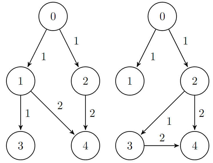
Figure 1: Interaction graphs $\mathcal{G}_{1}$ and $\mathcal{G}_{2}$

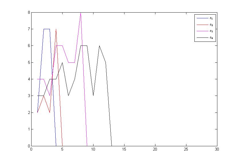
Figure 2: Errors between follower $i$ and the leader

V Conclusions

In this paper, we formulated a leader-following consensus problem of multi-agent systems over finite fields. Then we gave sufficient and/or necessary conditions for the agents to achieve the leader-following consensus. More general cases including general graph topology and multiple inputs for the consensus in finite fields are under investigation.

References

- [1] D. P. Bertsekas and J. N. Tsitsiklis, Parallel and Distributed Computation: Numerical Methods, Englewood Cliffs, 2003.
- [2] A. Das, R. Fierro, V. Kumar, J. Ostrowski, J. Spletzer and C. Taylor, A vision-based formation control framework. IEEE Transaction on Robotics and Automation, 18(5): 813–825, 2002.
- [3] B. Elspas, The theory of autonomous linear sequential networks, IRE Trans. Circuit Theory, 6(1): 45–60, 1959.
- [4] A. Fagiolini and A. Bicchi, On the robust synthesis of logical consensus algorithms for distributed intrusion detection, Automatica, 49(8): 2339–2550, 2013.
- [5] A. S. Fraenkel and Y. Yesha, Complexity of problems in games, graphs and algebraic equations, Discrete Applied Mathematics, 1(1-2): 15–30, 1979.
- [6] Y. Hong, J. Hu and L. Gao, Tracking control for multi-agent consensus with an active leader and variable topology, Automatica, 42(7): 1177–1182, 2006.
- [7] R. M. Jungers, The synchronizing probability function of an automaton. SIAM Journal on Discrete Mathematics, 26(1): 177–192, 2012.
- [8] R. E. Kalman, P. L. Falb and M. A. Arbib, Topics in mathematical system theory, New York: McGraw-Hill, 1969.
- [9] A. Kashyap, T. Basar and R. Srikant, Quantized consensus, Automatica, 43(7): 1192–1203, 2007.
- [10] D. B. Kingston and R. W. Beard, Discrete-time average-consensus under switching network topologies, American Control Conference, Minneapolis, 3551–3556, 2006.
- [11] R. Koetter and M. Medard, An algebraic approach to network coding, IEEE/ACM Trans Networking, 11(5): 782–795, 2003.
- [12] R. Lidl and H. Niederreiter, Finite Field, Cambridge University Press, 1996.
- [13] N. A. Lynch, Distributed Algorithms, San Francisco: Morgan Kaufmann Publishers Inc, 1996.
- [14] C. Ma and J. Zhang, Necessary and sufficient condtions for consensusability of linear multi-agent systems, IEEE Transaction on Automatic Control, 55(5): 1263–1268, 2010.
- [15] K. H. Movric, Y. You, F. L. Lewis and L. Xie, Synchronization of discrete-time multi-agent systems on graphs using Riccati design, Automatica, 49(2): 419–423, 2013.
- [16] W. Ni and D. Cheng, Leader-following consenus of multi-agent systems under fixed and switching topologies, System & Control Letters, 59: 209–217, 2010.
- [17] V. A. Nicholson, Matrices with permanent equal to one, Linear Algebra and its Applications, 12(2): 185–188, 1975.
- [18] R. Olfati-Saber, J. A. Fax and R. M. Murray, Consensus and cooperation in networked multi-agent systems, Proceedings of the IEEE, 95(1): 215–233, 2007.
- [19] F. Pasqualetti, D. Borra and F. Bullo, Consensus networks over finite fields, Automatica, 50(2): 349–358, 2014.
- [20] J. Reger, Linear systems over finite fields – modeling, analysis and synthesis, Ph.D. dissertation, University of Erlangen-Nuremberg, Nuremberg, Germany, 2004.
- [21] G. Shi and Y. Hong, Distributed coordination of multi-agent systems with switching structure and input saturation, IEEE Conference on Decision and Control, Shanghai, China, 895–900, 2009.
- [22] G. Shi, Y. Hong and K. Johansson, Connectivity and set tracking of multi-agent systems guided by multiple moving leaders, IEEE Transaction on Automatic Control, 57(3): 663–676, 2012.
- [23] S. Sundaram and C. N. Hadjicostis, Finite-time distributed consensus in graphs with time-invariant topologies, American Control Conference, New York, 711–716, 2007.
- [24] S. Sundaram and C. N. Hadjicostis, Structural controllability and observability of linear systems over finite fields with applications to multi-agent systems, IEEE Transaction on Automatic Control, 58(1): 60–73, 2013.
- [25] H. Tanner, G. Pappas and V. Kumar, Leader-to-formation stability, IEEE Transaction on Robotics and Automation, 20(3): 443–455, 2004.
- [26] R. A. H. Toledo, Linear finite dynamical systems, Communications in Algebra, 33(9): 2977–2089, 2005.
- [27] X. Xu and Y. Hong, Matrix approach to model matching of asynchronous sequential machines, IEEE Transaction on Automatic Control, 58(11): 2974–2979, 2013.
- [28] X. Xu and Y. Hong, Solvability and control design for synchronization of Boolean networks, Journal of Systems Science and Complexity, 36(6): 871–885, 2013.