Asymmetrically interacting spreading dynamics on complex layered networks

Abstract

The spread of disease through a physical-contact network and the spread of information about the disease on a communication network are two intimately related dynamical processes. We investigate the asymmetrical interplay between the two types of spreading dynamics, each occurring on its own layer, by focusing on the two fundamental quantities underlying any spreading process: epidemic threshold and the final infection ratio. We find that an epidemic outbreak on the contact layer can induce an outbreak on the communication layer, and information spreading can effectively raise the epidemic threshold. When structural correlation exists between the two layers, the information threshold remains unchanged but the epidemic threshold can be enhanced, making the contact layer more resilient to epidemic outbreak. We develop a physical theory to understand the intricate interplay between the two types of spreading dynamics.

Epidemic spreading Pastor-Satorras:2001 ; Tang:2009 ; Shu:2012 ; Wang:2013 ; Gross:2006 ; Holme:2012 and information diffusion Zanette:2002 ; Liu:2003 ; Zhou:2007 ; Noh:2004 are two fundamental types of dynamical processes on complex networks. While traditionally these processes have been studied independently, in real-world situations there is always coupling or interaction between them. For example, whether large-scale outbreak of a disease can actually occur depends on the spread of information about the disease. In particular, when the disease begins to spread initially, individuals can become aware of the occurrence of the disease in their neighborhoods and consequently take preventive measures to protect themselves. As a result, the extent of the disease spreading can be significantly reduced Funk:2010-2 ; Meloni:2011 ; Wang:2012 . A recent example is the wide spread of severe acute respiratory syndrome (SARS) in China in 2003, where many people took simple but effective preventive measures (e.g., by wearing face masks or staying at home) after becoming aware of the disease, even before it has reached their neighborhoods Tai:2007 . To understand how information spreading can mitigate epidemic outbreaks, and more broadly, the interplay between the two types of spreading dynamics has led to a new direction of research in complex network science Manfredi:2013 .

A pioneering step in this direction was taken by Funk et al., who presented an epidemiological model that takes into account the spread of awareness about the disease Funk:2009 ; Funk:2010-1 . Due to information diffusion, in a well-mixed population, the size of the epidemic outbreak can be reduced markedly. However, the epidemic threshold can be enhanced only when the awareness is sufficiently strong so as to modify the key parameters associated with the spreading dynamics such as the infection and recovery rates. A reasonable setting to investigate the complicated interplay between epidemic spreading and information diffusion is to assume two interacting network layers of of identical set of nodes, one for each type of spreading dynamics. Due to the difference in the epidemic and information spreading processes, the connection patterns in the two layers can in general be quite distinct. For the special case where the two-layer overlay networks are highly correlated in the sense that they have completely overlapping links and high clustering coefficient, a locally spreading awareness triggered by the disease spreading can raise the threshold even when the parameters in the epidemic spreading dynamics remain unchanged Funk:2009 ; Funk:2010-1 . The situation where the two processes spread successively on overlay networks was studied with the finding that the outbreak of information diffusion can constrain the epidemic spreading process Funk:2010-3 . An analytical approach was developed to provide insights into the symmetric interplay between the two types of spreading dynamics on layered networks Marceau:2011 . A model of competing epidemic spreading over completely overlapping networks was also proposed and investigated, revealing a coexistence regime in which both types of spreading can infect a substantial fraction of the network Karrer:2011 .

While the effect of information diffusion (or awareness) on epidemic spreading has attracted much recent interest Ahn:2006 ; Kiss:2010 ; Perra:2011 ; Sahneh:2012 ; Wu:2012 ; Ruan:2012 ; Jo:2006 ; Wang:2012_2 , many outstanding issues remain. In this paper we address the following three issues. The first concerns the network structures that support the two types of spreading dynamics, which were assumed to be identical in some existing works. However, in reality, the two networks can differ significantly in their structures. For example, in a modern society, information is often transmitted through electronic communication networks such as telephones Jiang:2013 and the Internet Faloutsos:1999 , but disease spreading usually takes place on a physical contact network Starnini:2013 . The whole complex system should then be modeled as a double-layer coupled network (overlay network or multiplex network) Buldyrev:2010 ; Gao:2012 ; Cozzo:2013 ; Kivela:2013 ; Kim:2013 , where each layer has a distinct internal structure and the interplay between between the two layers has diverse characteristics, such as inter-similarity Parshani:2010 , multiple support dependence Shao:2011 , and inter degree-degree correlation Lee:2012 , etc. The second issue is that the effects of one type of spreading dynamics on another are typically asymmetric Ahn:2006 , requiring a modification of the symmetric assumption used in a recent work Marceau:2011 . For example, the spread of a disease can result in elevated crisis awareness and thus facilitate the spread of the information about the disease Funk:2010-1 , but the spread of the information promotes more people to take preventive measures and consequently suppresses the epidemic spreading Ruan:2012 . The third issue concerns the timing of the two types of spreading dynamics because they usually occur simultaneously on their respective layers and affect each other dynamically during the same time period Marceau:2011 .

Existing works treating the above three issues separately showed that each can have some significant effect on the epidemic and information spreading dynamics Funk:2009 ; Marceau:2011 ; Mills:2013 . However, a unified framework encompassing the sophisticated consequences of all three issues is lacking. The purpose of this paper is to develop an asymmetrically interacting spreading-dynamics model to integrate the three issues so as to gain deep understanding into the intricate interplay between the epidemic and information spreading dynamics. When all three issues are taken into account simultaneously, we find that an epidemic outbreak on the contact layer can induce an outbreak on the communication layer, and information spreading can effectively raise the epidemic threshold, making the contact layer more resistant to disease spreading. When inter-layer correlation exists, the information threshold remains unchanged but the epidemic threshold can be enhanced, making the contact layer more resilient to epidemic outbreak. These results are established through analytic theory with extensive numerical support.

Results

In order to present our main results, we describe our two-layer network model and the dynamical process on each layer. We first treat the case where the double-layer networks are uncorrelated. We then incorporate layer-to-layer correlation in our analysis.

Model of communication-contact double-layer network. Communication-contact coupled layered networks are one class of multiplex networks Gomez:2013 . In such a network, an individual (a node) not only connects with his/her friends on a physical contact layer (subnetwork), but also communicates with them through the (electronic) communication layer. The structures of the two layers can in general be quite different. For example, an indoor-type of individual has few friends in the real world but may have many friends in the cyber space, leading to a much higher degree in the communication layer than in the physical-contact layer. Generally, the degree-to-degree correlation between the two layers cannot be assumed to be strong.

Our correlated network model of communication-contact layers is constructed, as follows. Two subnetworks $A$ and $B$ with the same node set are first generated independently, where $A$ and $B$ denote the communication and contact layers, respectively. Each layer possesses a distinct internal structure, as characterized by measures such as the mean degree and degree distribution. Then each node of layer $A$ is matched one-to-one with that of layer $B$ according to certain rules.

In an uncorrelated double-layer network, the degree distribution of one layer is completely independent of the distributions of other layer. For example, a hub node with a large number of neighbors in one layer is not necessarily a hub node in the other layer. In contrast, in a correlated double-layer network, the degree distributions of the two layers are strongly dependent upon each other. In a perfectly correlated double-layer network, hub nodes in one layer must simultaneously be hub nodes in the other layer. Quantitatively, the Spearman rank correlation coefficient Cho:2010 ; Lee:2012 $m_{s}$, where $m_{s}\in[-1,1]$ (see definition in Methods), can be used to characterize the degree correlation between the two layers. For $m_{s}>0$, the greater the correlation coefficient, the larger degree a pair of counterpart nodes can have. For $m_{s}<0$, as $|m_{s}|$ is decreased, a node of larger degree in one layer is matched with a node of smaller degree in the other layer.

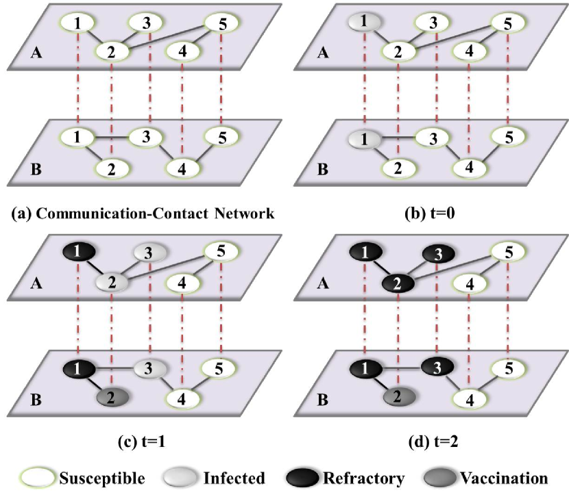
Figure 1: Illustration of asymmetrically coupled spreading processes on a simulated communication-contact double-layer network. (a) Communication and contact networks, denoted as layer $A$ and layer $B$, respectively, each of five nodes. (b) At $t=0$, node $B_{1}$ in layer $B$ is randomly selected as the initial infected node and its counterpart, node $A_{1}$ in layer $A$, gains the information that $B_{1}$ is infected, while all other pairs of nodes, one from layer $A$ and another from layer $B$, are in the susceptible state. (c) At $t=1$, within layer $A$ the information is transmitted from $A_{1}$ to $A_{2}$ with probability $\beta_{A}$. Node $B_{3}$ in layer $B$ can be infected by node $B_{1}$ with probability $\beta_{B}$ and, if it is indeed infected, its corresponding node $A_{3}$ in layer $A$ gets the information as well. Since, by this time, $A_{2}$ is already aware of the infection spreading, its counterpart $B_{2}$ in layer $B$ is vaccinated, say with probability $p$. At the same time, node $A_{1}$ in layer $A$ and its counterpart $B_{1}$ in layer $B$ enter into the refractory state with probability $\mu_{A}$ and $\mu_{B}$, respectively. (d) At $t=2$, all infected (or informed) nodes in both layers can no longer infect others, and start recovering from the infection. In both layers, the spreading dynamics terminate by this time.

Asymmetrically interacting spreading dynamics. The dynamical processes of disease and information spreading are typically asymmetrically coupled with each other. The dynamics component in our model can be described, as follows. In the communication layer (layer $A$), the classic susceptible-infected-recovered (SIR) epidemiological model Moreno:2002 is used to describe the dissemination of information about the disease. In the SIR model, each node can be in one of the three states: (1) susceptible state ($S$) in which the individual has not received any information about the disease, (2) informed state($I$), where the individual is aware of disease and is capable of transmitting the information to other individuals in the same layer, and (3) refractory state ($R$), in which the individual has received the information but is not willing to pass it on to other nodes. At each time step, the information can propagate from every informed node to all its neighboring nodes. If a neighbor is in the susceptible state, it will be informed with probability $\beta_{A}$. At the same time, each informed node can enter the recovering phase with probability $\mu_{A}$. Once an informed node is recovered, it will remain in this state for all subsequent time. A node in layer $A$ will get the information about the disease once its counterpart node in layer $B$ is infected. As a result, dissemination of the information over layer $A$ is facilitated by disease transmission on layer $B$.

The spreading dynamics in layer $B$ can be described by the SIRV model Ruan:2012 , in which a fourth sate, the state of vaccination ($V$), is introduced. Mathematically, the SIR component of the spreading dynamics is identical to the dynamics on layer $A$ except for different infection and recovery rates, denoted by $\beta_{B}$ and $\mu_{B}$, respectively. If a node in layer $B$ is in the susceptible state but its counterpart node in layer $A$ is in the infected state, the node in layer $B$ will be vaccinated with probability $p$. Disease transmission in the contact layer can thus be suppressed by dissemination of information in the communication layer. The two spreading processes and their dynamical interplay are illustrated schematically in Fig. 1. Without loss of generality, we set $\mu_{A}=\mu_{B}=1$.

Theory of spreading dynamics in uncorrelated double-layer networks. Two key quantities in the dynamics of spreading are the outbreak threshold and the fraction of infected nodes in the final steady state. We develop a theory to predict these quantities for both information and epidemic spreading in the double-layer network. In particular, we adopt the heterogeneous mean-field theory Barthelemy:2004 to uncorrelated double-layer networks.

Let $P_{A}(k_{A})$ and $P_{B}(k_{B})$ be the degree distributions of layers $A$ and $B$, with mean degree $\langle k_{A}\rangle$ and $\langle k_{B}\rangle$, respectively. We assume that the subnetworks associated with both layers are random with no degree correlation. The time evolution of the epidemic spreading is described by the variables $s_{k_{A}}^{A}(t)$, $\rho_{k_{A}}^{A}(t)$, and $r_{k_{A}}^{A}(t)$, which are the densities of the susceptible, informed, and recovered nodes of degree $k_{A}$ in layer $A$ at time $t$, respectively. Similarly, $s_{k_{B}}^{B}(t)$, $\rho_{k_{B}}^{B}(t),r_{k_{B}}^{B}(t)$, and $v_{k_{B}}^{B}(t)$ respectively denote the susceptible, infected, recovered, and vaccinated densities of nodes of degree $k_{B}$ in layer $B$ at time $t$.

The mean-field rate equations of the information spreading in layer $A$ are

$$\frac{ds_{k_{A}}^{A}(t)}{dt} = -s_{k_{A}}^{A}(t)[\beta_{A}k_{A}\Theta_{A}(t)+\beta_{B}\Theta_{B}(t)\sum_{k_{B}}k_{B}P_{B}(k_{B})],$$ (1)

$$\frac{d\rho_{k_{A}}^{A}(t)}{dt} = s_{k_{A}}^{A}(t)[\beta_{A}k_{A}\Theta_{A}(t)+\beta_{B}\Theta_{B}(t)\sum_{k_{B}}k_{B}P_{B}(k_{B})]-\rho_{k_{A}}^{A}(t),$$ (2)

$$\frac{dr_{k_{A}}^{A}(t)}{dt} = \rho_{k_{A}}^{A}(t).$$ (3)

The mean-field rate equations of epidemic spreading in layer $B$ are given by

$$\frac{ds_{k_{B}}^{B}(t)}{dt} = -s_{k_{B}}^{B}(t)\beta_{B}k_{B}\Theta_{B}(t)-p\beta_{A}\Theta_{A}(t)\sum_{k_{A}}s_{k_{A}}^{A}(t)k_{A}P_{A}(k_{A}),$$ (4)

$$\frac{d\rho_{k_{B}}^{B}(t)}{dt} = s_{k_{B}}^{B}(t)\beta_{B}k_{B}\Theta_{B}(t)-\rho_{k_{B}}^{B}(t),$$ (5)

$$\frac{dr_{k_{B}}^{B}(t)}{dt} = \rho_{k_{B}}^{B}(t),$$ (6)

$$\frac{dv_{k_{B}}^{B}(t)}{dt} = p\beta_{A}\Theta_{A}(t)\sum_{k_{A}}s_{k_{A}}^{A}(t)k_{A}P_{A}(k_{A}),$$ (7)

where $\Theta_{A}(t)$ ($\Theta_{B}(t)$) is the probability that a neighboring node in layer A (layer B) is in the informed (infected) state (See Methods for details).

From Eqs. (1)-(7), the density associated with each distinct state in layer $A$ or $B$ is given by

$$X_{h}(t)=\sum_{k_{h}=1}^{k_{h,max}}P_{h}(k_{h})X_{k_{h}}^{h}(t),$$ (8)

where $h\in\{A,B\}$, $X\in\{S,I,R,V\}$, and $k_{h,max}$ denotes the largest degree of layer $h$. The final densities of the whole system can be obtained by taking the limit $t\rightarrow\infty$.

Due to the complicated interaction between the disease and information spreading processes, it is not feasible to derive the exact threshold values. We resort to a linear approximation method to get the outbreak threshold of information spreading in layer $A$ (see Supporting Information for details) as

$$\beta_{Ac}=\left\{\begin{array}[]{l}\beta_{Au},\quad for\quad\beta_{B}\leq\beta_{Bu}\\ 0,\quad\quad for\quad\beta_{B}>\beta_{Bu},\end{array}\right.$$ (9)

where

$$\beta_{Au} \equiv \langle k_{A}\rangle/({\langle k_{A}^{2}\rangle-\langle k_{A}\rangle})\ \ \mbox{and}\ \$$

$$\beta_{Bu} \equiv \langle k_{B}\rangle/(\langle k_{B}^{2}\rangle-\langle k_{B}\rangle)$$

denote the outbreak threshold of information spreading in layer $A$ when it is isolated from layer $B$, and that of epidemic spreading in layer $B$ when the coupling between the two layers is absent, respectively.

Equation (9) has embedded within it two distinct physical mechanisms for information outbreak. The first is the intrinsic information spreading process on the isolated layer $A$ without the impact of the spreading dynamics from layer $B$. For $\beta_{B}>\beta_{Bu}$, the outbreak of epidemic will make a large number of nodes in layer $A$ “infected” with the information, even if on layer $A$, the information itself cannot spread through the population efficiently. In this case, the information outbreak has little effect on the epidemic spreading in layer $B$ because very few nodes in this layer are vaccinated. We thus have $\beta_{Bc}\approx\beta_{Bu}$ for $\beta_{A}\leq\beta_{Au}$.

However, for $\beta_{A}>\beta_{Au}$, epidemic spreading in layer $B$ is restrained by information spread, as the informed nodes in layer $A$ tend to make their counterpart nodes in layer $B$ vaccinated. Once a node is in the vaccination state, it will no longer be infected. In a general sense, vaccination can be regarded as a type of “disease,” as every node in layer $B$ can be in one of the two states: infected or vaccinated. Epidemic spreading and vaccination can thus be viewed as a pair of competing “diseases” spreading in layer $B$ Karrer:2011 . As pointed out by Karrer and Newman Karrer:2011 , in the limit of large network size $N$, the two competing diseases can be treated as if they were in fact spreading non-concurrently, one after the other.

Initially, both epidemic and vaccination spreading processes exhibit exponential growth (see Supporting Information). We can thus obtain the ratio of their growth rates as

$$\theta=\frac{\beta_{B}\beta_{Au}}{\beta_{A}\beta_{Bu}}.$$ (10)

For $\theta>1$, the epidemic disease spreads faster than the vaccination. In this case, the vaccination spread is insignificant and can be neglected. For $\theta<1$, information spreads much faster than the disease, in accordance with the situation in a modern society. Given that the vaccination and epidemic processes can be treated successively and separately, the epidemic outbreak threshold can be derived by a bond percolation analysis Newman:2005 ; Karrer:2011 (see details in Supporting Information). We obtain

$$\beta_{Bc}=\frac{\langle k_{B}\rangle}{(1-pS_{A})(\langle k_{B}^{2}\rangle-\langle k_{B}\rangle)},$$ (11)

where $S_{A}$ is the density of the informed population, which can be obtained by solving Eqs. (S18) and (S19) in Supporting Information. For $\theta<1$, we see from Eq. (11) that the threshold for epidemic outbreak can be enhanced by the following factors: strong heterogeneity in the communication layer, large information-transmission rate, and large vaccination rate.

Simulation results for uncorrelated networks. We use the standard configuration model to generate networks with power-law degree distributions Newman:2005-2 ; Newman:2001-2 ; Catanzaro:2005 for the communication subnetwork (layer A). The contact subnetwork in layer $B$ is of the Erdős and Rényi (ER) type Erdos:1959 . We use the notation SF-ER to denote the double-layer network. The sizes of both layers are set to be $N_{A}=N_{B}=2\times 10^{4}$ and their average degrees are $\langle k_{A}\rangle=\langle k_{B}\rangle=8$. The degree distribution of the communication layer is $P_{A}(k_{A})=\zeta k_{A}^{-{\gamma_{A}}}$ with the coefficient $\zeta=1/\sum_{k_{min}}^{k_{max}}k_{A}^{-{\gamma_{A}}}$ and the maximum degree $k_{max}\sim N^{1/({\gamma_{A}}-1)}$. We focus on the case of ${\gamma_{A}}=3.0$ here in the main text (the results for other values of the exponent, e.g., ${\gamma_{A}}=2.7$ and $3.5$, are similar, which are presented in Supporting Information). The degree distribution of the contact layer is $P_{B}(k_{B})=e^{-\langle k_{B}\rangle}\langle k_{B}\rangle^{k_{B}}/k_{B}!$. To initiate an epidemic spreading process, a node in layer $B$ is randomly infected and its counterpart node in layer $A$ is thus in the informed state, too. We implement the updating process with parallel dynamics, which is widely used in statistical physics Marro:1999 (see Sec. S3A in Supporting Information for more details). The spreading dynamics terminates when all infected nodes in both layers are recovered, and the final densities $R_{A}$, $R_{B}$, and $V_{B}$ are then recorded.

For epidemiological models [e.g., the susceptible-infected-susceptible (SIS) and SIR] on networks with a power-law degree distribution, the finite-size scaling method may not be effective to determine the critical point of epidemic dynamics Ferreira:2012 ; Hong:2007 , because the outbreak threshold depends on network size and it goes to zero in the thermodynamic limit Boguna:2013 ; Moreno:2002 . Therefore, we employ the susceptibility measure Ferreira:2012 $\chi$ to numerically determine the size-dependent outbreak threshold:

$$\chi=N\frac{\langle r^{2}\rangle-\langle r\rangle^{2}}{\langle r\rangle},$$ (12)

where $N$ is network size ($N=N_{A}=N_{B}$), and $r$ denotes the final outbreak ratio such as the final densities $R_{A}$ and $R_{B}$ of the recovered nodes in layers $A$ and $B$, respectively. We use $2\times 10^{3}$ independent dynamic realizations on a fixed double-layer network to calculate the average value of $\chi$ for the communication layer for each value of $\beta_{A}$. As shown in Fig. 2(a), $\chi$ exhibits a maximum value at $\beta_{Ac}$, which is the threshold value of the information spreading process. The simulations are further implemented using $30$ different two-layer network realizations to obtain the average value of $\beta_{Ac}$. The identical simulation setting is used for all subsequent numerical results, unless otherwise specified. Figure 2(b) shows the information threshold $\beta_{Ac}$ as a function of the disease-transmission rate $\beta_{B}$. Note that the statistical errors are not visible here (same for similar figures in the paper), as they are typically vanishingly small. We see that the behavior of the information threshold can be classified into two classes, as predicted by Eq. (9). In particular, for $\beta_{B}\leq\beta_{Bu}=1/\langle k_{B}\rangle=0.125$, the disease transmission on layer $B$ has little impact on the information threshold on layer $A$, as we have $\beta_{Ac}\approx\beta_{Au}=\langle k_{A}\rangle/({\langle k_{A}^{2}\rangle-\langle k_{A}\rangle})\approx 0.06$. For $\beta_{B}>\beta_{Bu}$, the outbreak of epidemic on layer $B$ leads to $\beta_{Ac}=0.0$. Comparison of the information thresholds for different vaccination rates shows that the value of the vaccination probability $p$ has essentially no effect on $\beta_{Ac}$.

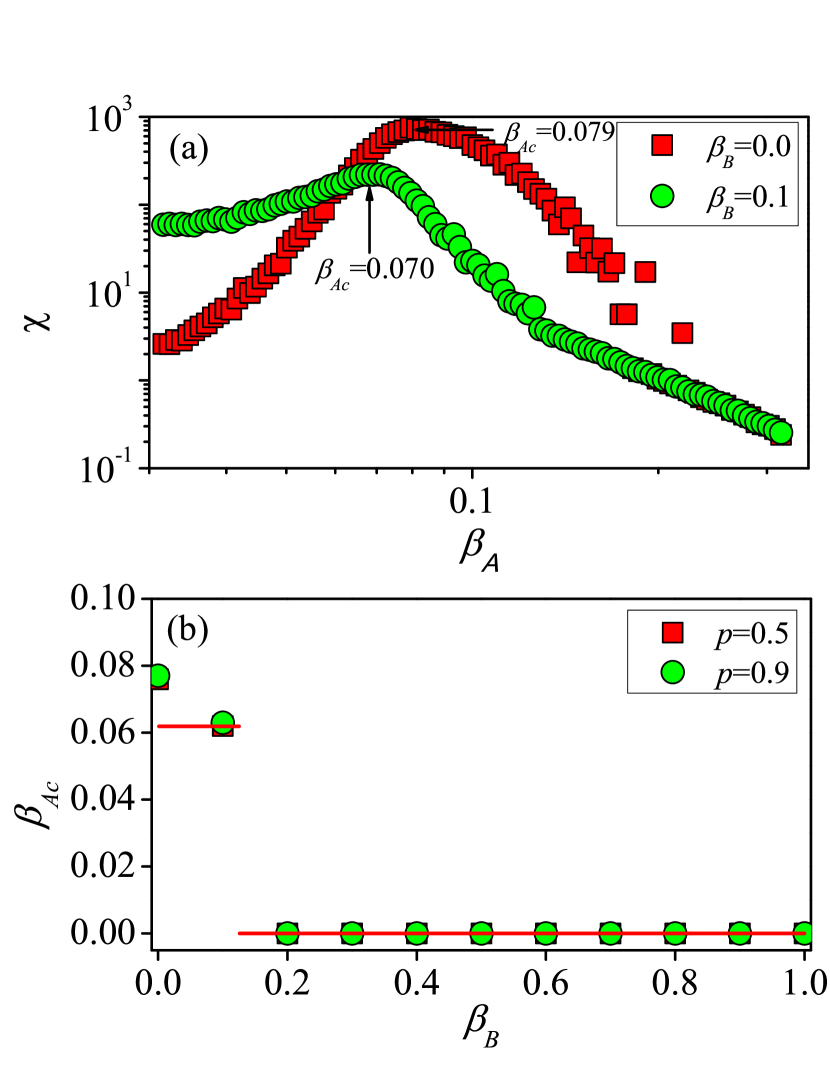
Figure 2: On SF-ER networks, (a) susceptibility measure $\chi$ as a function of the information-transmission rate $\beta_{A}$ for $p=0.5$, $\beta_{B}=0.0$ (red squares) and $\beta_{B}=0.1$ (green circles), (b) threshold $\beta_{Ac}$ of information spreading as a function of the disease-transmission rate $\beta_{B}$ for vaccination rate $p=0.5$ (red squares) and $p=0.9$ (green circles), where the red solid lines are analytical predictions from Eq. (9).

Figure 3 shows the effect of the information-transmission rate $\beta_{A}$ and the vaccination rate $p$ on the epidemic threshold $\beta_{Bc}$. From Fig. 3(a), we see that the value of $\beta_{Bc}$ is not influenced by $\beta_{A}$ for $\beta_{A}\leq\beta_{Au}\approx 0.06$, whereas $\beta_{Bc}$ increases with $\beta_{A}$. For $p=0.5$, the analytical results from Eq. (11) are consistent with the simulated results. However, deviations occur for larger values of $p$, e.g., $p=0.9$, because the effect of information spreading is over-emphasized in cases where the two types of spreading dynamics are treated successively but not simultaneously. The gap between the theoretical and simulated thresholds diminishes as the network size is increased, validating applicability of the analysis method that, strictly speaking, holds only in the thermodynamic limit Karrer:2011 (see details in Supporting Information). Note that a giant residual cluster does not exist in layer $B$ for $p=0.9$ and $\beta_{A}\geq 0.49$, ruling out epidemic outbreak. The phase diagram indicating the possible existence of a giant residual cluster [Eq. (S20) in Supporting Information] is shown in the inset of Fig. 3(a), where in phase II, there is no such cluster. In Fig. 3(b), a large value of $p$ causes $\beta_{Bc}$ to increase for $\beta_{A}>\beta_{Au}$. We observe that, similar to Fig. 3(a), for relatively large values of $p$, say $p\geq 0.8$, the analytical prediction deviates from the numerical results. The effects of network size $N$, exponent ${\gamma_{A}}$ and SF-SF network structure on the information and epidemic thresholds are discussed in detail in Supporting Information.

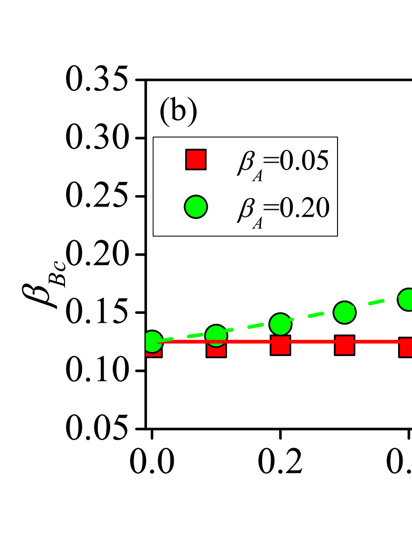
Figure 3: For SF-ER double-layer networks, epidemic threshold $\beta_{Bc}$ as a function of the information-transmission rate $\beta_{A}$ (a) and the vaccination rate $p$ (b). In (a), the red solid ($p=0.5$) and green dashed ($p=0.9$) lines are the analytical predictions from Eq. (11), and the blue dot-dashed line denotes the case of $\theta=1$ from Eq. (10). Iset of (a) shows the condition under which a giant residual cluster of layer $B$ exists [from Eq. (S20) in Supporting Information] in phase I. In (b), the red solid line ($\beta_{A}=0.05$) corresponds to $\beta_{Bc}=\beta_{Bu}$, and the green dashed line ($\beta_{A}=0.20$) is the analytical prediction from Eq. (11).

The final dynamical state of the double-layer spreading system is shown in Fig. 4. From Fig. 4(a), we see that the final recovered density $R_{A}$ for information increases with $\beta_{A}$ and $\beta_{B}$ rapidly for $\beta_{A}\leq\beta_{Au}$ and $\beta_{B}\leq\beta_{Bu}$. Figure 4(b) reveals that the recovered density $R_{B}$ for disease decreases with $\beta_{A}$. We see that a large value of $\beta_{A}$ can prevent the outbreak of epidemic for small values of $\beta_{B}$, as $R_{B}\rightarrow 0$ for $\beta_{B}=0.2$ and $\beta_{A}\geq 0.5$ (the red solid line). From Fig. 4(c), we see that, with the increase in $\beta_{A}$, more nodes in layer $B$ are vaccinated. It is interesting to note that the vaccinated density $V_{B}$ exhibits a maximum value if $\beta_{A}$ is not large. Figure 4 shows that the maximum value of $V_{B}$ is about $0.32$, which occurs at $\beta_{B}\approx 0.20$, for $\beta_{A}=0.2$. Combining with Fig. 3(a), we find that the corresponding point of the maximum value $\beta_{B}\approx 0.20$ is close to $\beta_{Bc}\approx 0.16$ for $p=0.5$. This is because the transmission of disease has the opposite effects on the vaccinations. For $\beta_{B}\leq\beta_{Bc}$, the newly infected nodes in layer $B$ will facilitate information spreading in layer $A$, resulting in more vaccinated nodes. For $\beta_{B}>\beta_{Bc}$, the epidemic spreading will make a large number of nodes infected, reducing the number of nodes that are potentially to be vaccinated. For relatively large values of $\beta_{A}$, information tends to spread much faster than the disease for $\beta_{B}\leq\beta_{Bc}$, e.g., $\theta\approx 0.21$ for $\beta_{A}=0.5$, $p=0.5$, $\beta_{Bc}\approx 0.22$, and $\theta\approx 0.12$ for $\beta_{A}=0.9$, $p=0.5$, and $\beta_{Bc}\approx 0.23$. In this case, the effect of disease transmission on information spreading is negligible. The densities of the final dynamical states for SF-SF networks are also shown in Supporting Information, and we observe similar behaviors.

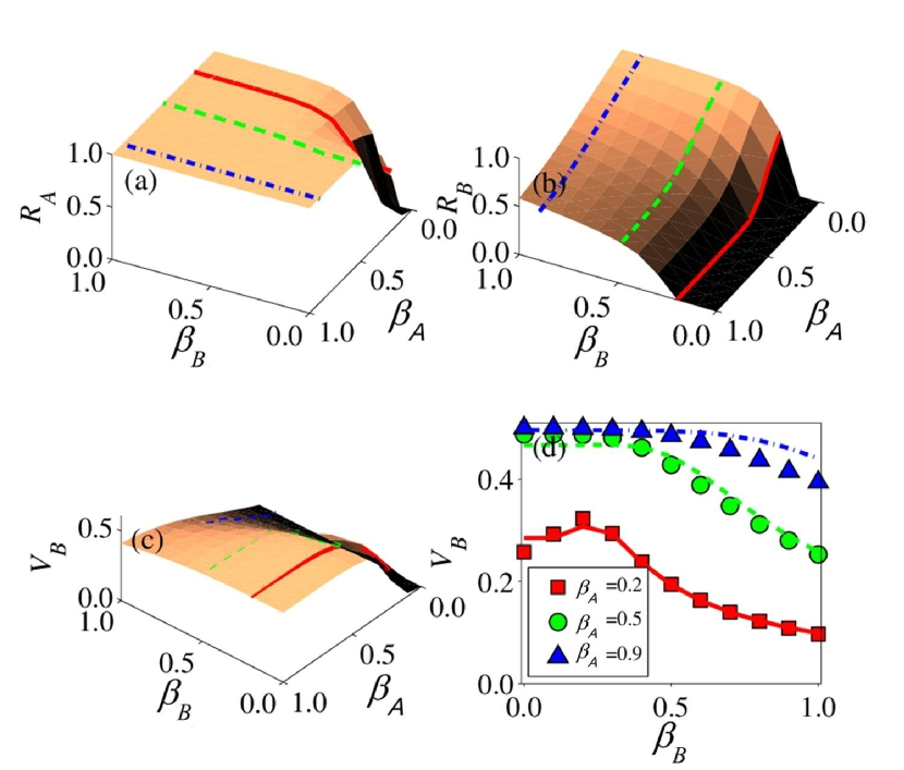
Figure 4: For SF-ER networks, final density in each state versus the parameters $\beta_{A}$ and $\beta_{B}$: (a) recovered density $R_{A}$, (b) recovered density $R_{B}$, (c) the vaccination density $V_{B}$, and (d) $V_{B}$ versus $\beta_{B}$ for $\beta_{A}=0.2,0.5,0.9$. The value of parameter $p$ is 0.5. Different lines are the numerical solutions of Eqs. (1)-(8) in the limit $t\rightarrow\infty$. In (a) and (d), we select three different values of $\beta_{A}$ (0.2, 0.5, and 0.9), corresponding to the red solid, green dashed, and blue dot-dashed lines, respectively. In (b) and (c), three different values of $\beta_{B}$ are chosen (0.2, 0.5, and 0.9), corresponding to the red solid, green dashed, and blue dot-dashed lines, respectively.

Spreading dynamics on correlated double-layer networks. In realistic multiplex networks certain degree of inter-layer correlations is expected to exist Kivela:2013 . For example, in social networks, positive inter-layer correlation is more common than negative correlation Szell:2010 ; Nicosia:2013 . That is, an “important” individual with a large number of links in one network layer (e.g., representing one type of social relations) tends to have many links in other types of network layers that reflect different kinds of social relations. Recent works have shown that inter-layer correlation can have a large impact on the percolation properties of multiplex networks Parshani:2010 ; Lee:2012 . Here, we investigate how the correlation between the communication and contact layers affects the information and disease spreading dynamics. To be concrete, we focus on the effects of positive correlation on the two types of spreading dynamics. It is necessary to construct a two-layer correlated network with adjustable degree of inter-layer correlation. This can be accomplished by first generating a two-layer network with the maximal positive correlation, where each layer has the same structure as uncorrelated networks. Then, $Nq$ pairs of counterpart nodes, in which $q$ is the rematching probability, are rematched randomly, leading to a two-layer network with weaker inter-layer correlation. The inter-layer correlation after rematching is given by (see Methods)

$$m_{s}\approx 1-q,$$ (13)

which is consistent with the numerical results [e.g., see inset of Fig. 5(a) below]. For SF-ER networks with fixed correlation coefficient, the mean-field rate equations of the double-layer system cannot be written down because the concrete expressions of the conditional probabilities $P(k_{B}|k_{A})$ and $P(k_{A}|k_{B})$ are no longer available.

We investigate how the rematching probability $q$ affects the outbreak thresholds in both the communication and epidemic layers. As shown in Fig. 5, we compare the case of $q=0.8$ with that of $q=0.0$. From Fig. 5(a), we see that $q$ has little impact on the outbreak threshold $\beta_{Ac}$ of the communication layer [with further support in Fig. 6(a), and analytic explanation using ER-ER correlated layered networks in Supporting Information]. We also see that the value of $\beta_{Ac}$ for ER-ER layered networks with the same mean degree is greater because of the homogeneity in the degree distribution of layer $A$. Figures 5(b) and 6(b) show that $\beta_{Bc}$ decreases with $q$ or, equivalently, $\beta_{Bc}$ increases with $m_{s}$. This is because stronger inter-layer correlation can increase the probability for nodes with large degrees in layer $B$ to be vaccinated, thus effectively preventing the outbreak of epidemic [see also Eqs. (S38)-(S41) in Supporting Information]. Figure 7 shows the final densities of different populations, providing the consistent result that, with the increase (decrease) of $q$ ($m_{s}$), the final densities $R_{A}$ and $R_{B}$ increase but the density $V_{B}$ decreases. For SF-SF networks, we obtain similar results (shown in Supporting Information).

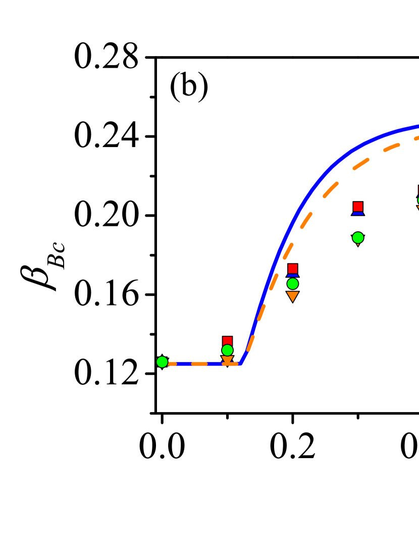
Figure 5: For two-layer correlated networks with vaccination probability $p=0.5$, the effect of one type of spreading dynamics on the outbreak threshold of the counter-type spreading dynamics. (a) $\beta_{Ac}$ versus $\beta_{B}$ on SF-ER networks with $q=0.0$ (red squares) and $q=0.8$ (green circles), and ER-ER networks with $q=0.0$ (blue up triangles) and $q=0.8$ (orange down triangles). Red solid (SF-ER) and blue dashed (ER-ER) lines are the analytical predictions from Eq. (9) and Eq. (S37) (in Supporting Information), respectively. The inset shows the inter-layer correlation $m_{s}$ as a function of rematching probability $q$. (b) $\beta_{Bc}$ versus $\beta_{A}$ on SF-ER networks with $q=0.0$ (red squares) and $q=0.8$ (green circles), and ER-ER networks with $q=0.0$ (blue up triangles) and $q=0.8$ (orange down triangles). Blue solid ($q=0.0$) and orange dashed ($q=0.8$) lines are the analytical predictions for ER-ER networks from Eqs. (S38)-(S41) in Supporting Information.

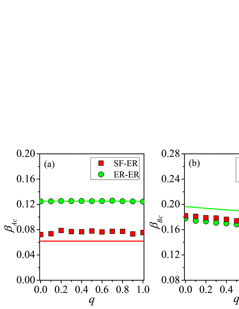
Figure 6: Effect of varying the rematching probability on outbreak thresholds of the two types of spreading dynamics. (a) $\beta_{Ac}$ versus $q$ on SF-ER (red squares) and ER-ER networks (green circles) for $\beta_{B}=0.05$ and $p=0.5$. Red Solid (SF-ER) and green dashed (ER-ER) lines are analytical predictions from Eq. (9) and Eq. (S37) in Supporting Information, respectively. (b) $\beta_{Bc}$ versus $q$ on SF-ER (red squares) and ER-ER networks (green circles) for $\beta_{A}=0.2$ and $p=0.5$. Green solid line is analytical prediction for ER-ER networks from Eqs. (S38)-(S41) in Supporting Information.

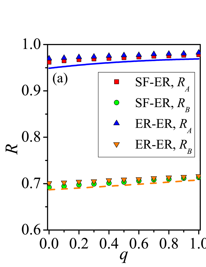
Figure 7: Effect of rematching probability on the final state. (a) $R_{A}$ versus $q$ on SF-ER (red squares) and ER-ER networks (blue up triangles), $R_{B}$ versus $q$ on SF-ER (green circles) and ER-ER networks (orange down triangles). (b) $V_{B}$ versus $q$ on SF-ER (red squares) and ER-ER networks (green circles). Different lines represent the analytic solutions for ER-ER networks, calculated by summing the final densities of all degrees from Eqs. (S28)-(S34) in Supporting Information. The parameter setting is $\beta_{A}=0.2$, $\beta_{B}=0.4$ and $p=0.5$.

Discussion

To summarize, we have proposed an asymmetrically interacting, double-layer network model to elucidate the interplay between information diffusion and epidemic spreading, where the former occurs on one layer (the communication layer) and the latter on the counterpart layer. A mean-field based analysis and extensive computations reveal an intricate interdependence of two basic quantities characterizing the spreading dynamics on both layers: the outbreak thresholds and the final fractions of infected nodes. In particular, on the communication layer, the outbreak of the information about the disease can be triggered not only by its own spreading dynamics but also by the the epidemic outbreak on the counter-layer. In addition, high disease and information-transmission rates can enhance markedly the final density of the informed or refractory population. On the layer of physical contact, the epidemic threshold can be increased but only if information itself spreads through the communication layer at a high rate. The information spreading can greatly reduce the final refractory density for the disease through vaccination. While a rapid spread of information will prompt more nodes in the contact layer to consider immunization, the authenticity of the information source must be verified before administrating large-scale vaccination.

We have also studied the effect of inter-layer correlation on the spreading dynamics, with the finding that stronger correlation has no apparent effect on the information threshold, but it can suppress the epidemic spreading through timely immunization of large-degree nodes Holme:2002 . These results indicate that it is possible to effectively mitigate epidemic spreading through information diffusion, e.g., by informing the high-centrality hubs about the disease.

The challenges of studying the intricate interplay between social and biological contagions in human populations are generating interesting science Bauch:2013 . In this work, we study asymmetrically interacting information-disease dynamics theoretically and computationally, with implications to behavior-disease coupled systems and articulation of potential epidemic-control strategies. Our results would stimulate further works in the more realistic situation of asymmetric interactions.

During the final writing of this paper, we noted one preprint posted online studying the dynamical interplay between awareness and epidemic spreading in multiplex networks Granell:2013 . In that work, the two competing infectious strains are described by two SIS processes. The authors find that the epidemic threshold depends on the topological structure of the multiplex network and the interrelation with the awareness process by using a Markov-chain approach. Our work thus provides further understanding and insights into spreading dynamics on multi-layer coupled networks.

Methods

Mean-Field theory for the uncorrelated double-layer networks. To derive the mean-field rate equations for the density variables, we consider the probabilities that node $A_{i}$ in layer $A$ and node $B_{i}$ in layer $B$ become infected during the small time interval $[t,t+dt]$. On the communication layer, a susceptible node $A_{i}$ of degree $k_{A}$ can obtain the information in two ways: from its neighbors in the same layer and from its counterpart node in layer $B$. For the first route, the probability that node $A_{i}$ receives information from one of its neighbors is $k_{A}\beta_{A}\Theta_{A}(t)dt$, where $\Theta_{A}(t)$ is the probability that a neighboring node is in the informed state Newman:2010 and is given by

$$\Theta_{A}(t)=\frac{\sum_{k_{A}^{\prime}}(k_{A}^{\prime}-1)P_{A}(k_{A}^{\prime})\rho_{k_{A}^{\prime}}^{A}(t)}{\langle k_{A}\rangle},$$ (14)

where $\langle k_{A}\rangle=\sum_{k_{A}}k_{A}P_{A}(k_{A})$. To model the second scenario, we note that, due to the asymmetric coupling between the two layers, a node in layer $A$ being susceptible requires that its counterpart node in layer $B$ be susceptible, too. A node in the communication layer will get the information about the disease once its counterpart node in layer $B$ is infected, which occurs with the probability $\sum_{k_{B}}P(k_{B}|k_{A})k_{B}\beta_{B}\Theta_{B}(t)dt$, where $P(k_{B}|k_{A})$ denotes the conditional probability that a node of degree $k_{A}$ in layer $A$ is linked to a node of degree $k_{B}$ in layer $B$, and $k_{B}\beta_{B}\Theta_{B}(t)dt$ is the probability for a counterpart node of degree $k_{B}$ to become infected in the time interval $[t,t+dt]$. If the subnetworks in both layers are not correlated, we have $P(k_{B}|k_{A})=P_{B}(k_{B})$. The mean-field rate equations of the information spreading in layer $A$ are Eqs. (1)-(3).

On layer $B$, a susceptible node $B_{i}$ of degree $k_{B}$ may become infected or vaccinated in the time interval $[t,t+dt]$. This can occur in two ways. Firstly, it may be infected by a neighboring node in the same layer with the probability $k_{B}\beta_{B}\Theta_{B}(t)dt$, where $\Theta_{B}(t)$ is the probability that a neighbor is in the infected state and is given by

$$\Theta_{B}(t)=\frac{\sum_{k_{B}^{\prime}}(k_{B}^{\prime}-1)P_{B}(k_{B}^{\prime})\rho_{k_{B}^{\prime}}^{B}(t)}{\langle k_{B}\rangle},$$ (15)

where $\langle k_{B}\rangle=\sum_{k_{B}}k_{B}P_{B}(k_{B})$. Secondly, if its counterpart node in layer $A$ has already received the information from one of its neighbors, it will be vaccinated with probability $p$. The probability for a node in layer $B$ to be vaccinated, taking into account the interaction between the two layers, is $p\sum_{k_{A}}P(k_{A}|k_{B})s_{k_{A}}^{A}(t)\beta_{A}k_{A}\Theta_{A}(t)dt$, where $P(k_{A}|k_{B})$ denotes the conditional probability that a node of degree $k_{B}$ in layer $B$ is linked to a node of degree $k_{A}$ in layer $A$, and $s_{k_{A}}^{A}(t)\beta_{A}k_{A}\Theta_{A}(t)dt$ is the informed probability for the counterpart node of degree $k_{A}$ in the susceptible state [$P(k_{A}|k_{B})=P_{A}(k_{A})$ for $m_{s}=0$]. The mean-field rate equations of epidemic spreading in layer $B$ are Eqs. (4)-(7). We note that the second term on the right side of Eq. (4) does not contain the variable $s_{k_{B}}^{B}(t)$ because a node in layer $B$ must be in the susceptible state if its counterpart node in layer $A$ is in the susceptible state.

Spearman rank correlation coefficient. The correlation between the layers can be quantified by the Spearman rank correlation coefficient Cho:2010 ; Lee:2012 defined as

$$m_{s}=1-6\frac{\sum_{i=1}^{N}\Delta_{i}^{2}}{N(N^{2}-1)},$$ (16)

where $N$ is network size and $\Delta_{i}$ denotes the difference between node $i$’s degrees in the two layers. When a node in layer $A$ is matched with a random node in layer $B$, $m_{s}$ is approximately zero in the thermodynamic limit. In this case, the double-layer network is uncorrelated Cho:2010 ; Lee:2012 . When every node has the same rank of degree in both layers, we have $m_{s}\approx 1$. In this case, there is a maximally positive inter-layer correlation where, for example, the hub node with the highest degree in layer $A$ is matched with the largest hub in layer $B$, and the same holds for the nodes with the smallest degree. In the case of maximally negative correlation, the largest hub in one layer is matched with a node having the minimal degree in the other layer, so we have $m_{s}\approx-1$.

In a double-layer network with the maximally positive correlation, any pair of nodes having the same rank of degree in the respective layers are matched, i.e., $\Delta_{i}=0$ for any pair of nodes $A_{i}$ and $B_{i}$. We thus have $m_{s}=1$, according to Eq. (16). After random rematching, a pair of nodes have $\Delta_{i}=0$ with probability $1-q$ and a random difference $\Delta_{i}^{\prime}$ with probability $q$. Equation (16) can then be rewritten as

$$m_{s}=1-6\frac{q\sum_{i=1}^{N}\Delta_{i}^{\prime 2}}{N(N^{2}-1)}.$$ (17)

When all nodes are randomly rematched, the layers in the network are completely uncorrelated, i.e., $m_{s}\approx 0$. In this case, we have

$$6\frac{\sum_{i=1}^{N}\Delta_{i}^{\prime 2}}{N(N^{2}-1)}\approx 1.$$ (18)

Submitting Eq. (18) into Eq. (17), the inter-layer correlation after rematching is given by

$$m_{s}\approx 1-q.$$ (19)

Figure legends

FIG 1: Illustration of asymmetrically coupled spreading processes on a simulated communication-contact double-layer network. (a) Communication and contact networks, denoted as layer $A$ and layer $B$, respectively, each of five nodes. (b) At $t=0$, node $B_{1}$ in layer $B$ is randomly selected as the initial infected node and its counterpart, node $A_{1}$ in layer $A$, gains the information that $B_{1}$ is infected, while all other pairs of nodes, one from layer $A$ and another from layer $B$, are in the susceptible state. (c) At $t=1$, within layer $A$ the information is transmitted from $A_{1}$ to $A_{2}$ with probability $\beta_{A}$. Node $B_{3}$ in layer $B$ can be infected by node $B_{1}$ with probability $\beta_{B}$ and, if it is indeed infected, its corresponding node $A_{3}$ in layer $A$ gets the information as well. Since, by this time, $A_{2}$ is already aware of the infection spreading, its counterpart $B_{2}$ in layer $B$ is vaccinated, say with probability $p$. At the same time, node $A_{1}$ in layer $A$ and its counterpart $B_{1}$ in layer $B$ enter into the refractory state with probability $\mu_{A}$ and $\mu_{B}$, respectively. (d) At $t=2$, all infected nodes in both layers can no longer infect others, and start recovering from the infection. In both layers, the spreading dynamics terminate by this time.

FIG 2: On SF-ER networks, (a) the susceptibility measure $\chi$ as a function of the information-transmission rate $\beta_{A}$ for $p=0.5$, $\beta_{B}=0.0$ (red squares) and $\beta_{B}=0.1$ (green circles), (b) the threshold $\beta_{Ac}$ of information spreading as a function of the disease-transmission rate $\beta_{B}$ for vaccination rate $p=0.5$ (red squares) and $p=0.9$ (green circles), where the red solid lines are analytical predictions from Eq. (9).

FIG 3: For SF-ER double-layer networks, epidemic threshold $\beta_{Bc}$ as a function of the information-transmission rate $\beta_{A}$ (a) and the vaccination rate $p$ (b). In (a), the red solid ($p=0.5$) and green dashed ($p=0.9$) lines are the analytical predictions from Eq. (11), and the blue dot-dashed line denotes the case of $\theta=1$ from Eq. (10). The inset of (a) shows the condition under which a giant residual cluster of layer $B$ exists [from Eq. (S20) in Supporting Information] in phase I. In (b), the red solid line ($\beta_{A}=0.05$) corresponds to $\beta_{Bc}=\beta_{Bu}$, and the green dashed line ($\beta_{A}=0.20$) is the analytical prediction from Eq. (11).

FIG 4: For SF-ER networks, the final density in each state versus the parameters $\beta_{A}$ and $\beta_{B}$: (a) recovered density $R_{A}$, (b) recovered density $R_{B}$, (c) the vaccination density $V_{B}$, and (d) $V_{B}$ versus $\beta_{B}$ for $\beta_{A}=0.2,0.5,0.9$. The value of parameter $p$ is 0.5. Different lines are the numerical solutions of Eqs. (1)-(8) in the limit $t\rightarrow\infty$. In (a) and (d), we select three different values of $\beta_{A}$ (0.2, 0.5, and 0.9), corresponding to the red solid, green dashed, and blue dot-dashed lines, respectively. In (b) and (c), three different values of $\beta_{B}$ are chosen (0.2, 0.5, and 0.9), corresponding to the red solid, green dashed, and blue dot-dashed lines, respectively.

FIG 5: For two-layer correlated networks with vaccination probability $p=0.5$, the effect of one type of spreading dynamics on the outbreak threshold of the counter-type spreading dynamics. (a) $\beta_{Ac}$ versus $\beta_{B}$ on SF-ER networks with $q=0.0$ (red squares) and $q=0.8$ (green circles), and ER-ER networks with $q=0.0$ (blue up triangles) and $q=0.8$ (orange down triangles). Red solid (SF-ER) and blue dashed (ER-ER) lines are the analytical predictions from Eq. (9) and Eq. (S37) (in Supporting Information), respectively. The inset shows the inter-layer correlation $m_{s}$ as a function of rematching probability $q$. (b) $\beta_{Bc}$ versus $\beta_{A}$ on SF-ER networks with $q=0.0$ (red squares) and $q=0.8$ (green circles), and ER-ER networks with $q=0.0$ (blue up triangles) and $q=0.8$ (orange down triangles). Blue solid ($q=0.0$) and orange dashed ($q=0.8$) lines are the analytical predictions for ER-ER networks from Eqs. (S38)-(S41) in Supporting Information.

FIG 6: Effect of varying the rematching probability on outbreak thresholds of the two types of spreading dynamics. (a) $\beta_{Ac}$ versus $q$ on SF-ER (red squares) and ER-ER networks (green circles) for $\beta_{B}=0.05$ and $p=0.5$. Red Solid (SF-ER) and green dashed (ER-ER) lines are analytical predictions from Eq. (9) and Eq. (S37) in Supporting Information, respectively. (b) $\beta_{Bc}$ versus $q$ on SF-ER (red squares) and ER-ER networks (green circles) for $\beta_{A}=0.2$ and $p=0.5$. Green solid line is analytical prediction for ER-ER networks from Eqs. (S38)-(S41) in Supporting Information.

FIG 7: Effect of rematching probability on the final state. (a) $R_{A}$ versus $q$ on SF-ER (red squares) and ER-ER networks (blue up triangles), $R_{B}$ versus $q$ on SF-ER (green circles) and ER-ER networks (orange down triangles). (b) $V_{B}$ versus $q$ on SF-ER (red squares) and ER-ER networks (green circles). Different lines represent the analytic solutions for ER-ER networks, calculated by summing the final densities of all degrees from Eqs. (S28)-(S34) in Supporting Information. The parameter setting is $\beta_{A}=0.2$, $\beta_{B}=0.4$ and $p=0.5$.

Author contributions

W. W., M. T. and Y. C. L devised the research project. W. W. and H. Y. performed numerical simulations. W. W., M. T., Y. H. D. and Y. C. L analyzed the results. W. W., M. T., Y. H. D., Y. C. L and GW. L wrote the paper.

Additional information

Competing financial interests: The authors declare no competing financial interests.

S1. Spreading dynamics on uncorrelated doubule-layer networks

We adopt the heterogeneous mean-field theory Barthelemy11:2004 to uncorrelated double-layer networks. Let $P_{A}(k_{A})$ and $P_{B}(k_{B})$ be the degree distributions of layers $A$ and $B$, with mean degree $\langle k_{A}\rangle$ and $\langle k_{B}\rangle$, respectively. We assume that the subnetworks associated with both layers are random with no degree correlation. The time evolution of the epidemic spreading is described by the variables $s_{k_{A}}^{A}(t)$, $\rho_{k_{A}}^{A}(t)$, and $r_{k_{A}}^{A}(t)$, which are the densities of the susceptible, infected, and recovered nodes of degree $k_{A}$ in layer $A$ at time $t$, respectively. Similarly, $s_{k_{B}}^{B}(t)$, $\rho_{k_{B}}^{B}(t),r_{k_{B}}^{B}(t)$, and $v_{k_{B}}^{B}(t)$ respectively denote the susceptible, infected, recovered, and vaccinated densities of nodes of degree $k_{B}$ in layer $B$ at time $t$.

A. Mean-field rate equations

The mean-field rate equations of the information spreading in layer $A$ are then

$$\frac{ds_{k_{A}}^{A}(t)}{dt}=-s_{k_{A}}^{A}(t)[\beta_{A}k_{A}\Theta_{A}(t)+\beta_{B}\Theta_{B}(t)\sum_{k_{B}}k_{B}P_{B}(k_{B})],$$

$$\frac{d\rho_{k_{A}}^{A}(t)}{dt}=s_{k_{A}}^{A}(t)[\beta_{A}k_{A}\Theta_{A}(t)+\beta_{B}\Theta_{B}(t)\sum_{k_{B}}k_{B}P_{B}(k_{B})]-\rho_{k_{A}}^{A}(t),$$

$$\frac{dr_{k_{A}}^{A}(t)}{dt}=\rho_{k_{A}}^{A}(t).$$

The mean-field rate equations of epidemic spreading in layer $B$ are thus given by

$$\frac{ds_{k_{B}}^{B}(t)}{dt}=-s_{k_{B}}^{B}(t)\beta_{B}k_{B}\Theta_{B}(t)-p\beta_{A}\Theta_{A}(t)\sum_{k_{A}}s_{k_{A}}^{A}(t)k_{A}P_{A}(k_{A}),$$

$$\frac{d\rho_{k_{B}}^{B}(t)}{dt}=s_{k_{B}}^{B}(t)\beta_{B}k_{B}\Theta_{B}(t)-\rho_{k_{B}}^{B}(t),$$

$$\frac{dr_{k_{B}}^{B}(t)}{dt}=\rho_{k_{B}}^{B}(t),$$

$$\frac{dv_{k_{B}}^{B}(t)}{dt}=p\beta_{A}\Theta_{A}(t)\sum_{k_{A}}s_{k_{A}}^{A}(t)k_{A}P_{A}(k_{A}),$$

where $\Theta_{A}(t)$ [$\Theta_{B}(t)$] is the probability that a neighboring node in layer A (layer B) is in the infected state.

From Eqs. (S1)-(S7), the density associated with each distinct state in layer $A$ or $B$ is given by

$$X_{h}(t)=\sum_{k_{h}=1}^{k_{h,max}}P_{h}(k_{h})X_{k_{h}}^{h}(t).$$

where $h\in\{A,B\}$, $X\in\{S,I,R,V\}$, and $k_{h,max}$ denotes the largest degree of layer $h$. The final densities of the whole system can be obtained by taking the limit $t\rightarrow\infty$.

B. Linear analysis for the information threshold

On an uncorrelated layered network, at the outset of the spreading dynamics, the whole system can be regarded as consisting of two coupled SI-epidemic subsystems Newman11:2010 with the time evolution described by Eqs. (S2) and (S5). For $t\rightarrow 0$, we have $s_{k_{A}}^{A}(t)\approx 1$ and $s_{k_{B}}^{B}(t)\approx 1$, which reduce Eqs. (S2) and (S5) to

$$\begin{cases}\frac{d\rho_{k_{A}}^{A}(t)}{dt}=\beta_{A}k_{A}\Theta_{A}(t)+\beta_{B}\langle k_{B}\rangle\Theta_{B}(t)-\rho_{k_{A}}^{A}(t),\\ \frac{d\rho_{k_{B}}^{B}(t)}{dt}=\beta_{B}k_{B}\Theta_{B}(t)-\rho_{k_{B}}^{B}(t).\end{cases}$$

For convenience, Eq. (S9) can be written concisely as

$$\frac{d\vec{\rho}}{dt}=C\vec{\rho}-\vec{\rho},$$

where the vector of infected density is defined as

$$\vec{\rho}\equiv(\rho_{k_{A}=1}^{A},\ldots,\rho_{k_{A,max}}^{A},\rho_{k_{B}=1}^{B},\ldots,\rho_{k_{B,max}}^{B})^{T},$$

and $C$ is a block matrix in the following form:

$$C=\left(\begin{array}[]{ccc}C^{A}&D^{B}\\ 0&C^{B}\\ \end{array}\right),$$

with matrix elements given by

$$C_{k_{A},k^{\prime}_{A}}^{A} = [\beta_{A}{k_{A}}({k^{\prime}_{A}}-1)P_{A}(k^{\prime}_{A})]/{\langle k_{A}\rangle},$$

$$C_{k_{B},k^{\prime}_{B}}^{B} = [\beta_{B}{k_{B}}({k^{\prime}_{B}}-1)P_{B}(k^{\prime}_{B})]/{\langle k_{B}\rangle},$$

$$D_{k_{B},k^{\prime}_{B}}^{B} = \beta_{B}({k^{\prime}_{B}}-1)P_{B}(k^{\prime}_{B}).$$

In general, information spreading on layer $A$ can be facilitated by the outbreak of the epidemic on layer $B$, as an infected node in layer $B$ instantaneously makes its counterpart node in layer $A$ “infected” with the information about the disease. This coupling effect, in combination with the intrinsic spreading dynamics on layer $A$, leads to more informed nodes in the communication layer than infected nodes on layer $B$. If the maximum eigenvalue $\Lambda_{C}$ of matrix $C$ is greater than $1$, an outbreak of the information will occur in the system Saumell-Mendiola11:2012 . We then have

$$\Lambda_{C}=\mbox{max}\{\Lambda_{A},\Lambda_{B}\},$$

where $\mbox{max}\{\}$ denotes the greater of the two, and

$$\Lambda_{A} = \beta_{A}(\langle k_{A}^{2}\rangle-\langle k_{A}\rangle)/\langle k_{A}\rangle,$$

$$\Lambda_{B} = \beta_{B}(\langle k_{B}^{2}\rangle-\langle k_{B}\rangle)/\langle k_{B}\rangle$$

are the maximum eigenvalues of matrices $C^{A}$ and $C^{B}$ Mieghem11:2011 , respectively. The outbreak threshold of information spreading in layer $A$ is given by

$$\beta_{Ac}=\left\{\begin{array}[]{l}\beta_{Au},\quad for\quad\beta_{B}\leq\beta_{Bu}\\ 0,\quad\quad for\quad\beta_{B}>\beta_{Bu}\end{array}\right.$$

where $\beta_{Au}\equiv\langle k_{A}\rangle/({\langle k_{A}^{2}\rangle-\langle k_{A}\rangle}$ and $\beta_{Bu}\equiv\langle k_{B}\rangle/(\langle k_{B}^{2}\rangle-\langle k_{B}\rangle$ denote the outbreak threshold of information spreading on layer $A$ when it is isolated from layer $B$, and that of epidemic spreading on layer $B$ when the coupling between the two layers is absent, respectively.

C. Competing percolation theory for epidemic threshold

To elucidate the interplay between epidemic and vaccination spreading, we must first determine which one is the faster “disease.” At the early time of the epidemic outbreak on the isolated layer $B$, the average number of infected nodes grows exponentially as

$$N_{e}=n_{0}R_{e}^{t}=n_{0}e^{t\ln R_{e}},$$

where $R_{e}=\beta_{B}/\beta_{Bu}$ is the basic reproductive number for the disease on the isolated layer $B$ Newman11:2002-2 , and $n_{0}$ denotes the number of initially infected nodes. Similarly, for information spreading on the isolated layer $A$, the average number of informed nodes at the early time is

$$N_{i}=n_{0}R_{i}^{t}=n_{0}e^{t\ln R_{i}},$$

where $R_{i}=\beta_{A}/\beta_{Au}$ is the reproductive number for information spreading on the isolated layer $A$. The resulting number of vaccinated nodes on layer $B$ is

$$N_{v}=pn_{0}R_{i}^{t}=pn_{0}e^{t\ln R_{i}}.$$

Since both epidemic and vaccination spreading processes exhibit exponential growth, we can obtain the ratio of their growth rates as

$$\theta=\frac{R_{e}}{R_{i}}=\frac{\beta_{B}\beta_{Au}}{\beta_{A}\beta_{Bu}}.$$

For $\theta>1$, i.e., $\beta_{B}\beta_{Au}>\beta_{A}\beta_{Bu}$, the epidemic disease spreads faster than the vaccination. In this case, the vaccination spread is insignificant and can be neglected.

To uncover the impact of information spreading on epidemic outbreak, we focus on the case of faster vaccination, i.e., $\theta<1$, in accordance with the fact that information always tends to spread much faster than epidemic in a modern society. Given that vaccination and epidemic can be treated successively and separately, the threshold of epidemic outbreak can be derived by a bond percolation analysis Newman11:2005 ; Karrer11:2011 .

Firstly, when information spreading on layer $A$ is over, the density of informed population is given by Newman11:2002-2

$$S_{A}=1-G_{A0}(u),$$

where $G_{A0}(x)=\sum_{k_{A}}P_{A}(k_{A})x^{k_{A}}$ is the generating function for the degree distribution of layer $A$, and $u$ is the probability that a node is not connected to the giant cluster via a particular one of its edges, which can be solved by

$$u=1-\beta_{A}+\beta_{A}G_{A1}(u),$$

where $G_{A1}(x)=\sum_{k_{A}}Q_{A}(k_{A})x^{k_{A}}$ is the generating function for the excess degree distribution, $Q_{A}(k_{A})=(k_{A}+1)P_{A}(k_{A}+1)/\langle k_{A}\rangle$, of layer $A$. Since $p$ is the probability that an informed node in layer $A$ makes its counterpart node in layer $B$ vaccinated, the number of vaccinated or removed nodes in layer $B$ is $pS_{A}$. A necessary condition for the outbreak of epidemic is the existence of a giant residual cluster in layer $B$ Gao11:2012 . We have

$$1-pS_{A}>f_{Bc}=\frac{1}{G_{B1}^{\prime}(1)},$$

where $G_{B1}(x)=\sum_{k_{B}}Q_{B}(k_{B})x^{k_{B}}$ is the generating function for the excess degree distribution, $Q_{B}(k_{B})=(k_{B}+1)P_{B}(k_{B}+1)/\langle k_{B}\rangle$, of layer $B$, and the prime denotes derivative. From Eq. (S20), we see that epidemic outbreak can occur only if $pS_{A}<1-1/G_{B1}^{\prime}(1)$.

The degree distribution of the residual network of layer $B$ is given by Cohen11:2001 ; Pastor-Satorras11:2002

$$\widetilde{P}_{B}(\widetilde{k}_{B})=f\sum_{k_{B}^{\prime}=\widetilde{k}_{B}}^{\infty}P_{B}(k_{B}^{\prime})\binom{k_{B}^{\prime}}{\widetilde{k}_{B}}(1-f)^{k_{B}^{\prime}-\widetilde{k}_{B}}f^{\widetilde{k}_{B}},$$

where $f=1-pS_{A}$ is the probability that a node is in the residual network. The generating function for the degree distribution of the residual network is then Newman11:2005

$$H_{B0}(x)=fG_{B0}(1-f+fx),$$

where $G_{B0}(x)=\sum_{k_{B}}P_{B}(k_{B})x^{k_{B}}$ is the generating function for the degree distribution of layer $B$. The generating function for its excess degree distribution is

$$H_{B1}(x)=\frac{H_{B0}^{\prime}(x)}{H_{B0}^{\prime}(1)}.$$

The basic reproductive number for a disease spreading over the residual network of layer $B$ is then given by Newman11:2002-2

$$\widetilde{R}_{i}=\beta_{B}H_{B1}^{\prime}(1).$$

The epidemic threshold corresponds to the point $\widetilde{R}_{i}=1$, and thus we have $\beta_{Bc}=1/H_{B1}^{\prime}(1)$. From Eqs. (S22)-(S24), we obtain the epidemic threshold $\beta_{Bc}$ as

$$\beta_{Bc}=\frac{\langle k_{B}\rangle}{(1-pS_{A})(\langle k_{B}^{2}\rangle-\langle k_{B}\rangle)},$$

where $S_{A}$ is the density of the informed population, which can be obtained by solving Eqs. (S18) and (S19).

S2. Spreading dynamics on correlated double-layer networks

We assume that layer $A$ has the same degree distribution as layer $B$. After a certain fraction $q$ of pairs of nodes, one from each layer, have been randomly rematched, the conditional probability $P(k_{B}|k_{A})$ can be written as

$$P(k_{B}|k_{A})=qP_{B}(k_{B})+(1-q)\delta_{k_{B},k_{A}},$$

or

$$P(k_{A}|k_{B})=qP_{A}(k_{A})+(1-q)\delta_{k_{A},k_{B}}.$$

A. Mean-field rate equations

Using Eqs. (S1)-(S3), we can write the mean-field rate equations for information spreading on layer $A$ as

$$\frac{ds_{k_{A}}^{A}(t)}{dt}=-s_{k_{A}}^{A}(t)\{\beta_{A}k_{A}\Theta_{A}(t)+\beta_{B}\Theta_{B}(t)\sum_{k_{B}}k_{B}[qP_{B}(k_{B})+(1-q)\delta_{k_{B},k_{A}}]\},$$

$$\frac{d\rho_{k_{A}}^{A}(t)}{dt}=s_{k_{A}}^{A}(t)\{\beta_{A}k_{A}\Theta_{A}(t)+\beta_{B}\Theta_{B}(t)\sum_{k_{B}}k_{B}[qP_{B}(k_{B})+(1-q)\delta_{k_{B},k_{A}}]\}-\rho_{k_{A}}^{A}(t),$$

$$\frac{dr_{k_{A}}^{A}(t)}{dt}=\rho_{k_{A}}^{A}(t).$$

Similarly, the mean-field rate equations for epidemic spreading on layer $B$ are

$$\frac{ds_{k_{B}}^{B}(t)}{dt}=-s_{k_{B}}^{B}(t)\beta_{B}k_{B}\Theta_{B}(t)-p\beta_{A}\Theta_{A}(t)\\ \sum_{k_{A}}s_{k_{A}}^{A}(t)k_{A}[qP_{A}(k_{A})+(1-q)\delta_{k_{A},k_{B}}],$$

$$\frac{d\rho_{k_{B}}^{B}(t)}{dt}=s_{k_{B}}^{B}(t)\beta_{B}k_{B}\Theta_{B}(t)-\rho_{k_{B}}^{B}(t),$$

$$\frac{dr_{k_{B}}^{B}(t)}{dt}=\rho_{k_{B}}^{B}(t),$$

$$\frac{dv_{k_{B}}^{B}(t)}{dt}=p\beta_{A}\Theta_{A}(t)\sum_{k_{A}}s_{k_{A}}^{A}(t)k_{A}[qP_{A}(k_{A})+(1-q)\delta_{k_{A},k_{B}}].$$

Substituting Eqs. (S28)-(S34) into Eq. (S8), we can get the density associated with each distinct state in layer $A$ or $B$.

B. Linear analysis for the information threshold

At the outset of the spreading dynamics, the whole system can be regarded as two coupled SI-epidemic subsystems Newman11:2010 with the time evolution described by Eqs. (S29) and (S32). In the limit $t\rightarrow 0$, we have $s_{k_{A}}^{A}(t)\approx 1$ and $s_{k_{B}}^{B}(t)\approx 1$. Equations (S29) and (S32) can then be reduced to

$$\begin{cases}\frac{d\rho_{k_{A}}^{A}(t)}{dt}=\beta_{A}k_{A}\Theta_{A}(t)+\beta_{B}[q\langle k_{B}\rangle+(1-q)k_{A}]\Theta_{B}(t)-\rho_{k_{A}}^{A}(t),\\ \frac{d\rho_{k_{B}}^{B}(t)}{dt}=\beta_{B}k_{B}\Theta_{B}(t)-\rho_{k_{B}}^{B}(t).\end{cases}$$

which can be written concisely as

$$\frac{d\vec{\rho}}{dt}=C\vec{\rho}-\vec{\rho},$$

where the matrix $C$ has the same form as in Eq. (S11) and

$$C_{k_{A},k^{\prime}_{A}}^{A} = [\beta_{A}{k_{A}}({k^{\prime}_{A}}-1)P_{A}(k^{\prime}_{A})]/{\langle k_{A}\rangle},$$

$$C_{k_{B},k^{\prime}_{B}}^{B} = [\beta_{B}{k_{B}}({k^{\prime}_{B}}-1)P_{B}(k^{\prime}_{B})]/{\langle k_{B}\rangle},$$

$$D_{k_{B},k^{\prime}_{B}}^{B} = \beta_{B}[q\langle k_{B}\rangle+(1-q)k_{A}]({k^{\prime}_{B}}-1)P_{B}(k^{\prime}_{B})/\langle k_{B}\rangle.$$

The threshold of information outbreak is given by

$$\beta_{Ac}=\left\{\begin{array}[]{l}\beta_{Au},\quad for\quad\beta_{B}\leq\beta_{Bu},\\ 0,\quad\quad for\quad\beta_{B}>\beta_{Bu},\end{array}\right.$$

which is the same as Eq. (9) in the main text. As described in uncorrelated networks, there are two distinct mechanisms that can lead to the outbreak of information on layer $A$, and these hold for correlated layered-networks as well. For $\beta_{B}\leq\beta_{Bu}$, only a small number of nodes in layer $B$ are infected, so the impact of the disease on information-outbreak threshold on layer $A$ is negligible. For $\beta_{B}>\beta_{Bu}$, epidemic spreading can result in the outbreak of information. In this case, the information-outbreak threshold is zero.

C. Competing percolation theory for epidemic threshold

For $\beta_{A}\leq\beta_{Au}$, information itself cannot spread through the population. There is thus hardly any effect of the information layer on the epidemic spreading on layer $B$, and we have $\beta_{Bc}\approx\beta_{Bu}$. But for $\beta_{A}>\beta_{Au}$, the effect of information spreading on the epidemic threshold cannot be ignored. To assess quantitatively the influence, we focus on the case of faster information spread, i.e., $\beta_{A}\beta_{Bu}>\beta_{B}\beta_{Au}$, rendering applicable a bond percolation analysis similar to uncorrelated networks. Specifically, after information spreads on layer $A$, the percentage of nodes that get the information is $S_{A}$, and the density of recovered nodes of degree $k_{A}$ is $r_{k_{A}}^{A}=1-u^{k_{A}}$, where $u$ is the probability that a node is not connected to the giant cluster by a particular edge [Eq. (S19)]. Vaccinating a number of counterpart nodes results in the random removal of some edges which connect the vaccinated nodes with the remaining nodes Cohen11:2001 ; Pastor-Satorras11:2002 . The probability $\widetilde{h}$ of an edge linking to a vaccinated node is

$$\widetilde{h}=\frac{p\sum_{k_{B}}[(1-q)r_{k_{A}}+qS_{A}]k_{B}P_{B}(k_{B})}{\langle k_{B}\rangle}.$$

The new degree distribution of the residual network on layer $B$ is thus given by

$$\widetilde{P}_{B}(\widetilde{k}_{B})=\sum_{k_{B}^{\prime}=\widetilde{k}_{B}}^{\infty}\{1-p[(1-q)r_{k_{A}}+qS_{A}]\}P_{B}(k_{B}^{\prime})\binom{k_{B}^{\prime}}{\widetilde{k}_{B}}(1-\widetilde{h})^{\widetilde{k}_{B}}{\widetilde{h}}^{k_{B}^{\prime}-\widetilde{k}_{B}}.$$

The requirement that a giant residual cluster exists is

$$\frac{\langle{\widetilde{k}_{B}}^{2}\rangle}{\langle\widetilde{k}_{B}\rangle}>2,$$

where $\langle\widetilde{k}_{B}\rangle$ and $\langle{\widetilde{k}_{B}}^{2}\rangle$ are the first and second moments of the degree distribution, respectively. Finally, we obtain the epidemic threshold as

$$\beta_{Bc}=\frac{\langle\widetilde{k}_{B}\rangle}{\langle\widetilde{k}_{B}^{2}\rangle-\langle\widetilde{k}_{B}\rangle}.$$

S3. Simulation results

We first describe the simulation process of the two spreading dynamics on double-layer networks, and then demonstrate the validity of the theoretical analysis on uncorrelated networks with different network sizes and degree exponents, finally, we present results for SF-SF correlated networks.

A. Simulation process

To initiate an epidemic spreading process, a node in layer $B$ is randomly infected and its counterpart node in layer $A$ is thus in the informed state, too. The updating process is performed with parallel dynamics, which is widely used in statistical physics Marro11:1999 . At each time step, we first calculate the informed (infected) probability $\pi_{A}=1-(1-\beta_{A})^{n_{I}^{A}}$ [$\pi_{B}=1-(1-\beta_{B})^{n_{I}^{B}}$] that each susceptible node in layer $A$ ($B$) may be informed (infected) by its informed (infected) neighbors, where $n_{I}^{A}$ ($n_{I}^{B}$) is the number of its informed (infected) neighboring nodes.

According to the dynamic mechanism, once node $A_{i}$ is in the susceptible state, its counterpart node $B_{i}$ will be also in the susceptible state. Considering the asymmetric coupling between the two layers in this case, both the information-transmission and disease-transmission events can hardly occur at the same time. Thus, with probability $\pi_{A}/(\pi_{A}+\pi_{B})$, node $A_{i}$ have a probability $\pi_{A}$ to get the information from its informed neighbors in layer $A$. If node $A_{i}$ is informed, its counterpart node $B_{i}$ will turn into the vaccination state with probability $p$. With probability $\pi_{B}/(\pi_{A}+\pi_{B})$, node $B_{i}$ have a probability $\pi_{B}$ to get the infection from its infected neighbors in layer $B$, and then node $A_{i}$ also get the information about the disease.

In the other case that node $B_{i}$ and its corresponding node $A_{i}$ are in the susceptible state and the informed (or refractory) state respectively, only the disease-transmission event can occur at the time step. Thus, node $B_{i}$ will be infected with probability $\pi_{B}$.

After renewing the states of susceptible nodes, each informed (infected) node can enter the recovering phase with probability $\mu_{A}=1.0$ ($\mu_{B}=1.0$). The spreading dynamics terminates when all informed (or infected) nodes in both layers are recovered, and the final densities $R_{A}$, $R_{B}$, and $V_{B}$ are then recorded. The simulations are implemented using $30$ different two-layer network realizations. The network size of $N_{A}=N_{B}=2\times 10^{4}$ and average degrees $\langle k_{A}\rangle=\langle k_{B}\rangle=8$ are used for all subsequent numerical results, unless otherwise specified.

B. Uncorrelated double-layer networks

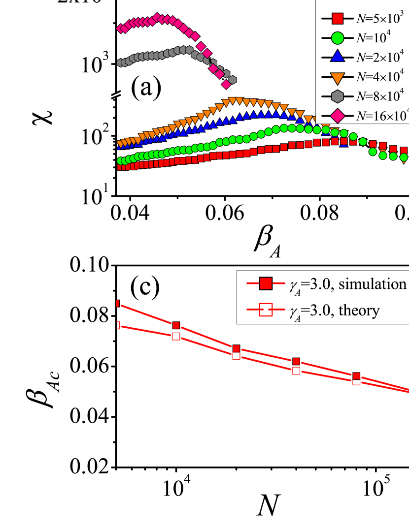
FIG. S 8: (Color online) On SF-ER networks, the susceptibility measure $\chi$ as a function of the information-transmission rate $\beta_{A}$ at $\beta_{B}=0.1$ (a) and the disease-transmission rate $\beta_{B}$ at $\beta_{A}=0.3$ (b) for $N=5\times 10^{3}$ (red squares), $N=10^{4}$ (green circles), $N=2\times 10^{4}$ (blue up triangles), $N=4\times 10^{4}$ (orange down triangles), $N=8\times 10^{4}$ (gray hexagons) and $N=16\times 10^{4}$ (pink diamonds); (c) the information threshold $\beta_{Ac}$ as a function of network size $N$ at $\beta_{B}=0.1$. (d) The epidemic threshold $\beta_{Bc}$ as a function of $N$ at $\beta_{A}=0.3$ for SF-ER networks (red solid squares) and SF-SF networks (green solid circles). The same hollow symbols represent the corresponding theoretical thresholds. The other parameters are the degree exponent $\gamma_{A}=3.0$ (or $\gamma_{B}=3.0$) and vaccination rate $p=0.5$.

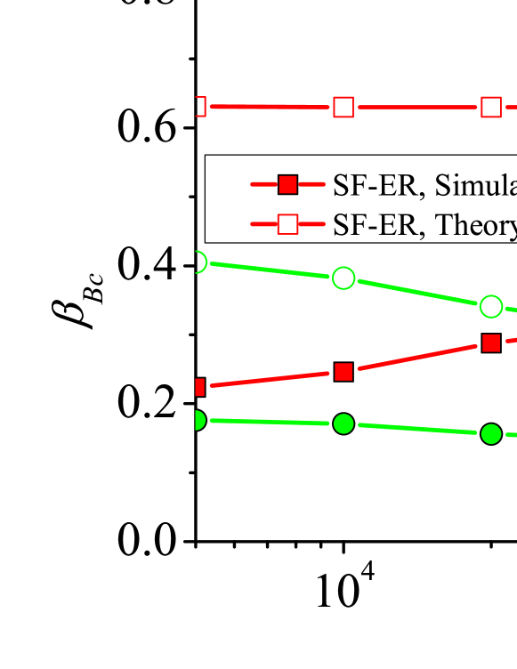
FIG. S 9: (Color online) The epidemic threshold $\beta_{Bc}$ as a function of network size $N$ for SF-ER networks (red solid squares) and SF-SF networks (green solid circles) at $\beta_{A}=0.3$ and $p=0.9$. The same hollow symbols represent the corresponding theoretical thresholds. For each SF layer, the degree exponent is set to $\gamma_{A}=3.0$ (or $\gamma_{B}=3.0$).

The effect of network size $N$ on the information and epidemic outbreak thresholds is first studied. According to Eq. (S13), the behavior of the information threshold can be classified into two classes. For $\beta_{B}\leq\beta_{Bu}$, the disease transmission on layer $B$ has little impact on the information threshold, as we have $\beta_{Ac}\approx\beta_{Au}=\langle k_{A}\rangle/({\langle k_{A}^{2}\rangle-\langle k_{A}\rangle})$; while $\beta_{Ac}=0.0$ for $\beta_{B}>\beta_{Bu}$. We here focus on the information threshold for $\beta_{B}\leq\beta_{Bu}$. From Figs.  S8(a) and (c), we see that the theoretical predictions are basically accordant with the simulated thresholds for different network sizes. With the growth of network size, the information threshold decreases as $\langle k^{2}\rangle$ of layer $A$ increases Boguna11:2013 . According to Eq. (S25), the theoretical epidemic threshold can be predicted. For SF-ER double-layer networks, Figs. S8(b) and (d) shows that the simulated epidemic thresholds deviate slightly from the theoretical predictions. However, the larger deviations occur for the larger values of the vaccination rate $p$, e.g., $p=0.9$ in Fig. S9, because the basic assumption of competing percolation theory is not strictly correct for the finite-size networks. As pointed out by Karrer and Newman Karrer11:2011 , in the limit of large network size $N$, the vaccination and epidemic processes can be treated successively and separately. On the double-layer networks with finite network size, the effect of information spreading is somewhat over-emphasized. From Figs. S8 and S9, we also see that the discrepancy between the simulated and theoretical thresholds decreases with network size $N$.

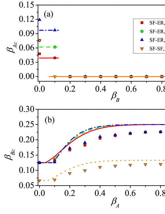
FIG. S 10: (Color online) On various double-layer networks, $\beta_{Ac}$ versus $\beta_{B}$ (a) and $\beta_{Bc}$ versus $\beta_{A}$ (b) for the SF-ER networks with $\gamma_{A}=2.7$ (red squares), the SF-ER networks with $\gamma_{A}=3.0$ (green circles), the SF-ER networks with $\gamma_{A}=3.5$ (blue up triangles) and the SF-SF networks with $\gamma_{A}=\gamma_{B}=3.0$ (orange down triangles). The analytical predictions of $\beta_{Ac}$ and $\beta_{Bc}$ are from Eq. (S13) and Eq. (S25), respectively. The vaccination rate is set to $p=0.5$.

We then investigate how the degree heterogeneity of layer $A$ influences the information and epidemic outbreak thresholds by adjusting the exponent $\gamma_{A}$. The information thresholds for the different exponents of layer $A$ are compared in Fig. S10(a), and the stronger heterogeneity of layer $A$ (i.e., smaller $\gamma_{A}$) can more easily make the information outbreak. Fig. S10(b) shows that increasing the heterogeneity of layer $A$ can slightly raise the epidemic threshold $\beta_{Bc}$ at a small information-transmission rate $\beta_{A}$, while making for the epidemic outbreak at a large $\beta_{A}$. This phenomenon results from the different effects of the heterogeneity on the information spreading under different transmission rates. The more homogeneous degree distribution does not always hinder the diffusion of information, especially at a large transmission rate Pastor-Satorras11:2001 ; Pastor-Satorras11:2002 .

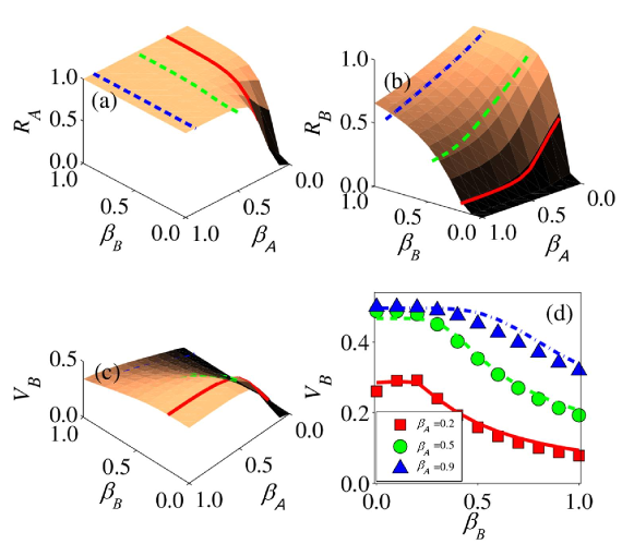
FIG. S 11: (Color online) For SF-SF networks, the final density in each state versus the parameters $\beta_{A}$ and $\beta_{B}$: (a) recovered density $R_{A}$, (b) recovered density $R_{B}$, (c) the vaccination density $V_{B}$, and (d) $V_{B}$ versus $\beta_{B}$ for $\beta_{A}=0.2,0.5,0.9$. The other parameter are $p=0.5$ and $\gamma_{A}=\gamma_{B}=3.0$. Different lines are the numerical solutions of Eqs. (S1)-(S8) in the limit $t\rightarrow\infty$. In (a) and (d), we select three different values of $\beta_{A}$ (0.2, 0.5, and 0.9), corresponding to the red solid, green dashed, and blue dot-dashed lines, respectively. In (b) and (c), three different values of $\beta_{B}$ are chosen (0.2, 0.5, and 0.9), corresponding to the red solid, green dashed, and blue dot-dashed lines, respectively.

To further demonstrate the validity of the theoretical analysis, we consider the case of SF-SF double-layer networks. Similar to the case of SF-ER networks, the gap between the theoretical and simulated thresholds is narrowing with the increase of network size [see Figs. S8(d) and S9], which implies the reasonability of the assumption in the thermodynamic limit. The final dynamical state of the SF-SF spreading system is also shown in Fig. S11, and it displays a similar phenomenon to the case of SF-ER networks. We also see that the theoretical predictions from mean-field rate equations are in good agreement with the simulation results.

C. Correlated double-layer networks

On SF-SF correlated networks, we investigate the effect of positive inter-layer correlation on the two types of spreading dynamics. As shown in Figs. S12, S13 and S14, with the increase of the correlation $m_{s}$ (by reducing the rematching probability $q$), the information threshold remains unchanged but the epidemic threshold can be enhanced, making the contact layer more robust to epidemic outbreak, which is consistent with the results for ER-ER correlated networks.

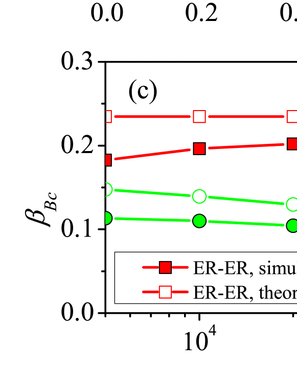
FIG. S 12: (Color online) On double-layer networks, (a) $\beta_{Ac}$ versus $\beta_{B}$, (b) $\beta_{Bc}$ versus $\beta_{A}$, and (c) $\beta_{Bc}$ versus $N$ at $\beta_{A}=0.3$. In (a) and (b), red solid squares and green solid circles respectively denote the simulation results for $q=0.0$ and $q=0.8$ on SF-SF networks, and the lines are the corresponding theoretical thresholds. In (c), the value of parameter $q$ is $0.0$, solid red squares and solid green circles respectively represent the results for ER-ER and SF-SF networks, and the same shapes are the corresponding theoretical predictions. The other parameter are $p=0.5$ and $\gamma_{A}=\gamma_{B}=3.0$.

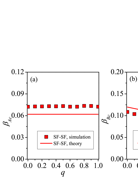
FIG. S 13: (Color online) On SF-SF networks, the effect of varying the rematching probability on outbreak thresholds of the two types of spreading dynamics. (a) $\beta_{Ac}$ versus $q$ for $\beta_{B}=0.05$ and $p=0.5$. Red Solid line is the analytical prediction from Eq. (S37). (b) $\beta_{Bc}$ versus $q$ for $\beta_{A}=0.2$ and $p=0.5$. Red solid line is the analytical prediction from Eqs. (S38)-(S41). The value of degree exponent is $\gamma_{A}=\gamma_{B}=3.0$.

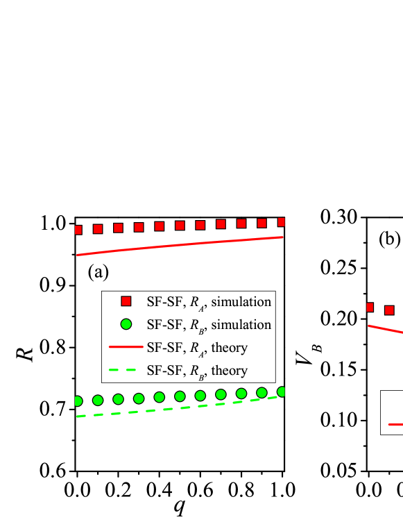
FIG. S 14: (Color online) On SF-SF networks, the effect of rematching probability on the final state. (a) $R_{A}$ versus $q$ (red squares) and $R_{B}$ versus $q$ (green circles), (b) $V_{B}$ versus $q$ (red squares). Different lines represent the analytic solutions for SF-SF networks, calculated by summing the final densities of all degrees from Eqs. (S28)-(S34). The parameter setting is $\gamma_{A}=\gamma_{B}=3.0,\beta_{A}=0.2$, $\beta_{B}=0.4$ and $p=0.5$.

References

- (1) Pastor-Satorras, R. & Vespignani, A. Epidemic Spreading in Scale-Free Networks. Phys. Rev. Lett. 86, 3200 (2001).
- (2) Tang, M, Liu, Z., & Li, B. Epidemic spreading by objective traveling. Europhys. Lett. 87, 18005 (2009).
- (3) Shu, P., Tang, M., Gong, K., & Liu, Y. Effects of weak ties on epidemic predictability on community networks. Chaos 22, 043124 (2012).
- (4) Wang, L., Wang, Z., Zhang, Y., & Li, X. How human location-specific contact patterns impact spatial transmission between populations? Sci. Rep. 3, 1468 (2013).
- (5) Gross, T, Dommar D’Lima, C. & Blasius, B. Epidemic dynamics on an adaptive network. Phys. Rev. Lett. 96, 208701 (2006).
- (6) Holme, P. & Sarama̋ki, J. Temporal networks, Phys. Rep. 519, 97-125 (2012).
- (7) Zanette, D. H. Dynamics of rumor propagation on small-world networks. Phys. Rev. E 65, 041908 (2002).
- (8) Liu, Z., Lai, Y. C., & Ye, N. Propagation and immunization of infection on general networks with both homogeneous and heterogeneous components. Phys. Rev. E 67, 031911 (2003).
- (9) Noh, J. D., & Rieger, H. Random Walks on Complex Networks. Phys. Rev. Lett. 92, 118701 (2004).
- (10) Zhou, J., Liu, Z. & Li, B. Influence of network structure on rumor propagation. Phys. Lett. A 368, 458 (2007).
- (11) Funk, S. Salathé, M. & Jansen, V. A. A. Modelling the influence of human behaviour on the spread of infectious diseases: a review. J. R. Soc. Interface 7, 1257-1274 (2010).
- (12) Meloni, S., Perra, N., Arenas, A., Gómez, S., Moreno, Y. & Vespignani, A. Modeling human mobility responses to the large-scale spreading of infectious diseases. Sci. Rep. 1, 62 (2011).
- (13) Wang, B., Cao, L., Suzuki, H. & Aihara, K. Safety-information-driven human mobility patterns with metapopulation epidemic dynamics, Sci. Rep. 2, 887 (2012).
- (14) Tai, Z. & Sun, T. Media dependencies in a changing media environment: The case of the 2003 SARS epidemic in China. New. Media. Soc. 9, 987-1010 (2007).
- (15) Manfredi, P. & D’Onofrio, A. Modeling the Interplay Between Human Behavior and the Spread of Infectious Diseases (Springer-Verlag, Berlin, 2013).
- (16) Funk, S., Gilada, E., Watkinsb, C., & Jansen, V. A. A. The spread of awareness and its impact on epidemic outbreaks. Proc. Natl. Acad. Sci. 106, 6872 (2009).
- (17) Funk, S., Gilad, E. & Jansen, V. A. A. Endemic disease, awareness, and local behavioural response. J. Theor. Biol 264, 501-509(2010).
- (18) Funk, S. & Jansen, V. A. A. Interacting epidemics on overlay networks. Phys. Rev. E 81, 036118 (2010).
- (19) Marceau, V., Noël, P. A., Hébert-Dufresne, L., Allard, A. & Dubé, L. J. Modeling the dynamical interaction between epidemics on overlay networks. Phys. Rev. E 84, 026105 (2011).
- (20) Karrer, B. & Newman, M. E. J. Competing epidemics on complex networks. Phys. Rev. E 84, 036106 (2011).
- (21) Ahn, Y. -Y., Jeong, H., Masuda, N. & Noh, J. D. Epidemic dynamics of two species of interacting particles on scale-free networks. Phys. Rev. E 74, 066113 (2006).
- (22) Kiss, I. Z., Cassell, J., Recker, M., & Simon, P. L. The impact of information transmission on epidemic outbreaks. Math. Biosci. 225, 1-10 (2010).
- (23) Perra, N., Balcan, D., Gonçalves, B. & Vespignani, A. Towards a Characterization of Behavior-Disease Models. PLoS ONE 6, e23084 (2011).
- (24) Sahneh, F. D., Chowdhury, F. N., & Scoglio, C. M. On the existence of a threshold for preventive behavioral responses to suppress epidemic spreading. Sci. Rep. 2, 632 (2012).
- (25) Wu, Q., Fu, X., Small, M., & Xu, X. J. The impact of awareness on epidemic spreading in networks. Chaos 22, 013101 (2012).
- (26) Ruan, Z., Tang, M. & Liu, Z. Epidemic spreading with information-driven vaccination. Phys. Rev. E 86, 036117 (2012).
- (27) Jo, H.-H., Baek, S.K. & Moon, H.-T. Immunization dynamics on a two-layer network model. Physica A 361, 534-542 (2006).
- (28) Wang, B., Cao, L, Suzuki, H. & Aihara, K. Impacts of clustering on interacting epidemics. J. Theor. Biol., 304, 121-130 (2012).
- (29) Jiang, Z. Q., Xie, W. J., Li, M. X., Podobnik, B., Zhou, W. X. & Stanley, H. E. Calling patterns in human communication dynamics. Proc. Natl. Acad. Sci. 110, 1600 (2013).
- (30) Faloutsos, M., Faloutsos, P., & Faloutsos, C. On power-law relationships of the Internet topology. Comput. Commun. Rev. 29, 251 (1999).
- (31) Starnini, M., Baronchelli, A. & Pastor-Satorras, R. Modeling Human Dynamics of Face-to-Face Interaction Networks. Phys. Rev. Lett. 110, 168701 (2013).
- (32) Buldyrev, S. V., Parshani, R., Paul, G., Stanley, H. E. & Havlin, S. Catastrophic cascade of failures in interdependent Networks. Nature (London) 464, 1025 (2010).
- (33) Gao, J., Buldyrev, S. V., Stanley, H. E. & Havlin, S. Networks formed from interdependent networks. Nat. Phys. 8, 40-48 (2012).
- (34) Cozzo, E., Baños, R. A., Meloni, S. & Moreno, Y. Contact-based social contagion in multiplex networks. Phys. Rev. E 88, 050801(R) (2013).
- (35) Kivelä, M., Arenas, A., Barthelemy, M., Gleeson, J. P., Moreno, Y. & Porter, M. A. Multilayer Networks. arXiv:1309.7233v1 (2013).
- (36) Kim,J. Y & Goh, K.-I. Coevolution and Correlated Multiplexity in Multiplex Networks. Phys. Rev. Lett. 111, 058702 (2013).
- (37) Parshani, R., Rozenblat, C., Ietri, D., Ducruet, C., & Havlin, S. Inter-similarity between coupled networks. Europhys. Lett. 92, 68002 (2010).
- (38) Shao, J., Buldyrev, S. V., Havlin, S. & Stanley, H. E. Cascade of failures in coupled network systems with multiple support-dependence relations. Phys. Rev. E 83, 036116 (2011).
- (39) Lee, K.-M., Kim, J. Y., Cho, W. -K., Goh, K. -I. & Kim, I. -M. Correlated multiplexity and connectivity of multiplex random networks. New J. Phys. 14, 033027 (2012).
- (40) Mills, H. L., Ganesh, A. & Colijn, C. Pathogen spread on coupled networks: effect of host and network properties on transmission thresholds. J. Theor. Biol. 320, 47 (2013).
- (41) Gómez, S., Díaz-Guilera, A., Gómez-Gardeñes, J., Pérez-Vicente, C. J., Moreno, Y. & Arenas, A. Diffusion Dynamics on Multiplex Networks. Phys. Rev. Lett. 110, 028701 (2013).
- (42) Cho, W.-K., Goh, K.-I. & Kim, I.-M. Correlated couplings and robustness of coupled networks. arXiv:1010.4971 (2010).
- (43) Moreno, Y., Pastor-Satorras, R. & Vespignani, A. Epidemic outbreaks in complex heterogeneous networks. Eur. Phys. J. B 26, 521-529 (2002).
- (44) Barthélemy, M., Barrat, A., Pastor-Satorras, R. & Vespignani, A. Velocity and Hierarchical Spread of Epidemic Outbreaks in Scale-Free Networks. Phys. Rev. Lett. 92, 178701 (2004).
- (45) Newman, M. E. J. Threshold Effects for Two Pathogens Spreading on a Network. Phys. Rev. Lett. 95, 108701 (2005).
- (46) Newman, M. E. J. Power laws, Pareto distributions and Zipf’s law. Contemp. Phys. 46, 323-351 (2005).
- (47) Catanzaro, M., Boguñá, M. & Pastor-Satorras, R. Generation of uncorrelated random scale-free networks. Phys. Rev. E 71, 027103 (2005).
- (48) Newman, M. E. J., Strogatz, S. H. & Watts, D. J. Random graphs with arbitrary degree distributions and their applications. Phys. Rev. E 64, 026118 (2001).
- (49) Erdős, P. & Rényi, On random graphs. Publ. Math. 6, 290-297 (1959).
- (50) Marro, J. & Dickman, R. Nonequilibrium Phase Transitions in Lattice Models (Cambridge University Press, Cambridge, 1999).
- (51) Hong, H., Ha, M. & Park, H. Finite-Size Scaling in Complex Networks. Phys. Rev. Lett. 98, 258701 (2007).
- (52) Ferreira, S. C., Castellano, C. & Pastor-Satorras, R. Epidemic thresholds of the susceptible-infected-susceptible model on networks: A comparison of numerical and theoretical results. Phys. Rev. E 86, 041125 (2012).
- (53) Bogũá, M., Castellano, C. & Pastor-Satorras, R. Nature of the epidemic threshold for the susceptible-infected-susceptible dynamics in networks. Phys. Rev. Lett. 111, 068701 (2013).
- (54) Szell, M., Lambiotte, R. & Thurner, S. Multirelational Organization of Large-scale Social Networks in an Online World. Proc. Natl. Acad. Sci. 107, 13636 (2010).
- (55) Nicosia, V., Bianconi, G., Latora, V. & Barthelemy, M. Growing Multiplex Networks. Phys. Rev. Lett. 111, 058701 (2013).
- (56) Holme, P., Kim, B. J., Yoon, C. N. & Han, S. K. Attack vulnerability of complex networks. Phys. Rev. E 65, 056109 (2002).
- (57) Bauch, C. T., & Galvani, A. P. Social Factors in Epidemiology. Science 342, 4 (2013).
- (58) C. Granell, S. Gómez, and A. Arenas. Dynamical interplay between awareness and epidemic spreading in multiplex networks. Phys. Rev. Lett. 111, 128701 (2013).
- (59) Newman, M. E. J. Networks An Introduction (Oxford University Press, Oxford, 2010).

References

- (1) Barthélemy, M., Barrat, A., Pastor-Satorras, R. & Vespignani, A. Velocity and Hierarchical Spread of Epidemic Outbreaks in Scale-Free Networks. Phys. Rev. Lett. 92, 178701 (2004).
- (2) Newman, M. E. J. Networks An Introduction (Oxford University Press, Oxford, 2010).
- (3) Saumell-Mendiola, A., Ángeles Serrano, M. & Boguñá, M. Epidemic spreading on interconnected networks. Phys. Rev. E 86, 026106 (2012).
- (4) Mieghem, P. V. Graph Spectra for Complex Networks (Cambrige university press, England, 2011).
- (5) Newman, M. E. J. Spread of epidemic disease on networks. Phys. Rev. E 66, 016128 (2002).
- (6) Newman, M. E. J. Threshold Effects for Two Pathogens Spreading on a Network. Phys. Rev. Lett. 95, 108701 (2005).
- (7) Karrer, B. & Newman, M. E. J. Competing epidemics on complex networks.Phys. Rev. E 84, 036106 (2011).
- (8) Gao, J., Buldyrev, S. V., Stanley, H. E. & Havlin,S. Networks formed from interdependent networks. Nat. Phys. 8, 40-48 (2012).
- (9) Cohen, R., Erez, K., ben-Avraham, D., & Havlin, S. Breakdown of the Internet under Intentional Attack. Phys. Rev. Lett. 86, 3682 (2001).
- (10) Pastor-Satorras, R. & Vespignani, A. Immunization of complex networks. Phys. Rev. E 65, 036104 (2002).
- (11) Marro, J. & Dickman, R. Nonequilibrium Phase Transitions in Lattice Models (Cambridge University Press, Cambridge, 1999).
- (12) Boguñá, M., Castellano, C. & Pastor-Satorras, R. Nature of the Epidemic Threshold for the Susceptible-Infected-Susceptible Dynamics in Networks. Phys. Rev. Lett. 111, 068701 (2013).
- (13) Pastor-Satorras, R., & Vespignani, A. Epidemic dynamics and endemic states in complex networks. Phys. Rev. E 63, 066117 (2001).