Abstract

We present an analytic expression of the nonperturbative free energy of a double-well supersymmetric matrix model in its double scaling limit, which corresponds to two-dimensional type IIA superstring theory on a nontrivial Ramond-Ramond background. To this end we draw upon the wisdom of random matrix theory developed by Tracy and Widom, which expresses the largest eigenvalue distribution of unitary ensembles in terms of a Painlevé II transcendent. Regularity of the result at any value of the string coupling constant shows that the third-order phase transition between a supersymmetry-preserving phase and a supersymmetry-broken phase, previously found at the planar level, becomes a smooth crossover in the double scaling limit. Accordingly, the supersymmetry is always broken spontaneously as its order parameter stays nonzero for the whole region of the coupling constant. Coincidence of the result with the unitary one-matrix model suggests that one-dimensional type 0 string theories partially correspond to the type IIA superstring theory. Our formulation naturally allows for introduction of an instanton chemical potential, and reveals the presence of a novel phase transition, possibly interpreted as condensation of instantons.

1 Introduction

Spontaneous supersymmetry (SUSY) breaking in superstring theory is one of crucial phenomena for superstrings to describe our real world. Although various matrix models have been investigated as nonperturbative formulations of superstring/M theory [1, 2, 3, 4, 5, 6], it is still difficult to elucidate whether these models do break SUSY and derive our four-dimensional world. In this situation, a simple double-well SUSY matrix model had been recently considered in [7, 8], and its connection to two-dimensional type IIA superstring theory [9] on a nontrivial Ramond-Ramond background had been explored from the viewpoint of symmetries [10] and from direct comparison of scattering amplitudes at the tree and one-loop orders [11]. Interestingly, in a double scaling limit that realizes the type IIA superstring theory, instanton effects of the matrix model survive and break the SUSY spontaneously [12]. This suggests that the corresponding type IIA superstring theory nonperturbatively breaks its target-space SUSY. Further investigation along this direction is expected to give insights to nonperturbative SUSY breaking in realistic superstring theory.

In this paper, the nonperturbative computation of the free energy of the SUSY matrix model is completed by drawing upon the result of Tracy and Widom [13, 14] on the distribution of the largest eigenvalue in random matrix theory . Consequently we shall find that the full nonperturbative free energy is expressed in terms of a Painlevé II transcendent, in coincidence with the unitary one-matrix model [24]. It suggests correspondence between two-dimensional $U(N)$ gauge theory and some sector of the two-dimensional IIA superstring theory, as well as partial equivalence of the IIA superstrings to one-dimensional type 0 strings. The expression is regular for the whole region of the coupling constant, and allows expansions in both regions of weak and strong string coupling constants. In particular, the third-order phase transition between the SUSY phase and the SUSY-broken phase previously found in a simple large-$N$ limit (planar limit) disappears in the double scaling limit. As a bonus of our method, the free energy or the partition function is naturally generalized by introducing instanton fugacity $\xi$. The original free energy or partition function is reproduced as $\xi\to 1$.

This paper is organized as follows. Our SUSY matrix model is briefly reviewed in the next section, and relevant random matrix techniques are summarized in section 3. By combining contents in the above two sections, we present the nonperturbative free energy in section 4. In section 5, the generalized free energy is shown to exhibit a phase transition due to condensation of instantons at an arbitrarily small string coupling constant. Section 6 is devoted to summarize the results obtained so far and present some of future directions. In appendix A, we present some technical steps to the result of Tracy and Widom relevant to the text.

2 SUSY double-well matrix model

The SUSY double-well matrix model is defined by the zero-dimensional reduction of a Wess-Zumino type action with superpotential $W(\phi)=\frac{1}{3}\phi^{3}-\mu^{2}\phi$:

$$S=N{\rm tr}\left[\frac{1}{2}B^{2}+iB(\phi^{2}-\mu^{2})+\bar{\psi}(\phi\psi+\psi\phi)\right],$$ (1)

where $B$ and $\phi$ are $N\times N$ hermitian matrices, and $\psi$ and $\bar{\psi}$ are $N\times N$ Grassmann-odd matrices. $S$ is invariant under SUSY transformations generated by $Q$ and $\bar{Q}$:

$$Q\phi=\psi,\quad Q\psi=0,\quad Q\bar{\psi}=-iB,\quad QB=0,$$ (2)

$$\bar{Q}\phi=-\bar{\psi},\quad\bar{Q}\bar{\psi}=0,\quad\bar{Q}\psi=-iB,\quad\bar{Q}B=0,$$ (3)

which leads to the nilpotency: $Q^{2}=\bar{Q}^{2}=\{Q,\bar{Q}\}=0$. In the planar limit (large-$N$ limit with $\mu^{2}$ fixed), the theory has two phases – (I) SUSY phase for $\mu^{2}>2$ and (II) SUSY-broken phase for $\mu^{2}<2$. The phase (I) has infinitely degenerate minima parametrized by filling fraction $(\nu_{+},\nu_{-})$ , and transition between the phases (I) and (II) is of the third order [7, 8]. As discussed in [10, 11, 12], various correlation functions of the two-dimensional type IIA superstring theory compactified on $\mathbb{R}\times S^{1}$ at the selfdual radius, with the string coupling $g_{s}$ and the Liouville coupling $\omega$ (multiplied by the tachyon operator), coincide with their counterparts in this matrix model through the identification $g_{s}=N^{-1}$ and $4\omega=\mu^{2}-2$, in the double scaling limit

$$N\to\infty\quad\mbox{and}\quad\mu^{2}\to 2+0\quad\mbox{with}\quad s=N^{2/3}(\mu^{2}-2)\,=g_{s}^{-2/3}\cdot 4\omega\quad\mbox{fixed}$$ (4)

from the phase (I). Thus, the weakly and strongly coupled regions of the IIA superstrings correspond to $s\gg 1$ and $0<s\ll 1$, respectively. The strength of the Ramond-Ramond background is expressed in terms of $\nu_{+}-\nu_{-}$. After integrating out the auxiliary field $B$ and the fermionic fields $\psi$ and $\bar{\psi}$, the partition function of the matrix model can be recast as integrals with respect to $N$ eigenvalues $\{\lambda\}=\{\lambda_{1},\ldots,\lambda_{N}\}$ of $\phi$:

$$Z(\mu^{2})=\tilde{C}_{N}\int_{-\infty}^{\infty}\prod_{i=1}^{N}\left(d\lambda_{i}\,e^{-NV(\lambda_{i})}\right)\triangle_{N}(\{\lambda\})^{2}\prod_{j,k=1}^{N}(\lambda_{j}+\lambda_{k}),$$ (5)

where $\triangle_{N}(\{\lambda\}):=\prod_{i>j}^{N}(\lambda_{i}-\lambda_{j})$, $V(\lambda)=\frac{1}{2}(\lambda^{2}-\mu^{2})^{2}$, and $1/\tilde{C}_{N}=(2\pi)^{\frac{N}{2}}N^{-\frac{N^{2}}{2}}\prod_{k=0}^{N}k!$. The integration region of each eigenvalue is divided into the positive and negative real axes, and the partition function associated with the filling fraction $(\nu_{+},\nu_{-})$, denoted by $Z_{(\nu_{+},\nu_{-})}(\mu^{2})$, is defined by integrations over the positive real axis for the first $\nu_{+}N$ eigenvalues and over the negative real axis for the remaining $\nu_{-}N$. Then, it is easy to see the relation $Z_{(\nu_{+},\nu_{-})}(\mu^{2})=(-1)^{\nu_{-}N}\,Z_{(1,0)}(\mu^{2})$, where

$$Z_{(1,0)}(\mu^{2})=\tilde{C}_{N}\int_{0}^{\infty}\prod_{i=1}^{N}\left(d\lambda_{i}\,e^{-NV(\lambda_{i})}\right)\triangle_{N}(\{\lambda\})^{2}\prod_{j,k=1}^{N}(\lambda_{j}+\lambda_{k}).$$ (6)

The total partition function with a regularization parameter $\alpha$ is defined by

$$Z_{\alpha}(\mu^{2})=\sum_{\nu_{-}N=0}^{N}\frac{N!}{(\nu_{+}N)!(\nu_{-}N)!}\,e^{-i\alpha\nu_{-}N}Z_{(\nu_{+},\nu_{-})}(\mu^{2})=(1-e^{-i\alpha})^{N}\,Z_{(1,0)}(\mu^{2}).$$ (7)

The one-point function $\langle\frac{1}{N}{\rm tr}(iB)\rangle_{\alpha}$ normalized by $Z_{\alpha}(\mu^{2})$ coincides with $\langle\frac{1}{N}{\rm tr}(\phi^{2}-\mu^{2})\rangle^{(1,0)}$ normalized by $Z_{(1,0)}(\mu^{2})$. This is well-defined in the limit $\alpha\to 0$ and serves as an order parameter of spontaneous SUSY breaking.

The partition function in the $(1,0)$ sector (6) can be cast in an alternative form by a change of variables $\lambda_{i}\mapsto x_{i}=\mu^{2}-\lambda_{i}^{2}$:

$$Z_{(1,0)}(\mu^{2})=\tilde{C}_{N}\int^{\mu^{2}}_{-\infty}\prod_{i=1}^{N}\left(dx_{i}\,e^{-\frac{N}{2}x_{i}^{2}}\right)\triangle_{N}(\{x\})^{2}$$ (8)

Using this expression, one- and two-instanton effects to the one-point function and $Z_{(1,0)}(\mu^{2})$ are analytically obtained in [12], from which spontaneous breaking of SUSY by instantons is concluded. Full nonperturbative contributions are also numerically computed up to $N=10^{6}$, and these results are extrapolated to $N=\infty$. One of the aims of this article is to present an analytic form of full nonperturbative contributions to $Z_{(1,0)}(\mu^{2})$ by recalling results in random matrix theory.

3 Gap probability of GUE

Here we collect some basic facts related to the celebrated result of Tracy and Widom [13, 14] for completeness. For an ensemble of sets of $N$ real numbers $\{x\}=\{x_{1},\ldots,x_{N}\}$, we consider a joint probability distribution (j.p.d.) $P(\{x\})$ which is totally symmetric under the exchange of any two entries and normalized by $\int_{\mathbb{R}}\prod_{i=1}^{N}dx_{i}\,P(\{x\})=1$. Let us also introduce a function associated with an interval $I\subset\mathbb{R}$ by

$$\tau(\xi;I):=\int_{\mathbb{R}}\prod_{i=1}^{N}dx_{i}(1-\xi\chi_{I}(x_{i}))\,P(\{x\}).$$ (9)

Here the characteristic function of $I$ is denoted by $\chi_{I}(\cdot)$, i.e. $\chi_{I}(x)=1$ for $x\in I$, and $\chi_{I}(x)=0$ otherwise. In power series expansion of (9) with respect to $(-\xi)$, the coefficient of $(-\xi)^{k}$ represents a probability in which any $k$ elements of $\{x\}$ are in $I$ and the remaining $(N-k)$ unrestricted (namely, at least $k$ elements are in $I$). On the other hand, in expansion with respect to $(1-\xi)$, the coefficient of $(1-\xi)^{k}$ gives a probability of exactly $k$ elements belonging in $I$, due to $1-\xi\chi_{I}(x)=\chi_{\mathbb{R}\backslash I}(x)+(1-\xi)\chi_{I}(x)$. These are expressed by the formula:

$$\tau(\xi;I)=1+\sum_{k=1}^{N}\frac{(-\xi)^{k}}{k!}\int_{I}dx_{1}\cdots dx_{k}R_{k}(x_{1},\ldots,x_{k})=\sum_{k=0}^{N}(1-\xi)^{k}E_{k}(I),$$ (10)

where

$$R_{k}(x_{1},\ldots,x_{k})=\frac{N!}{(N-k)!}\int_{\mathbb{R}}dx_{k+1}\cdots dx_{N}\,P(\{x\})$$ (11)

is the $k$-point correlation function, and

$$E_{k}(I)=\left({N\atop k}\right)\int_{I}dx_{1}\cdots dx_{k}\int_{\mathbb{R}\backslash I}dx_{k+1}\cdots dx_{N}\,P(\{x\})$$ (12)

is the probability distribution of $k$ elements exclusively in $I$. In particular, at $\xi=1$ it is equal to the ‘gap probability’ that the all $x_{i}$’s lie outside the interval $I$,

$$\tau(1;I)=E_{0}(I)=\int_{\mathbb{R}\backslash I}\prod_{i=1}^{N}dx_{i}\,P(\{x\}).$$ (13)

3.1 Hermitian random matrices

For an ensemble of $N\times N$ Hermitian random matrices $M$ defined by the partition function of the one-matrix model

$$Z_{\rm 1MM}=\int d^{N^{2}}M\,e^{-{\rm tr}\,U(M)}=\tilde{C}_{N}\int_{\mathbb{R}}\prod_{i=1}^{N}\left(dx_{i}\,e^{-U(x_{i})}\right)\triangle_{N}(\{x\})^{2},$$ (14)

the corresponding j.p.d. is

$$P(\{x\})=\frac{\tilde{C}_{N}}{Z_{\rm 1MM}}\,\prod_{i=1}^{N}e^{-U(x_{i})}\triangle_{N}(\{x\})^{2}.$$ (15)

This j.p.d. and the $k$-point correlation function $R_{k}(x_{1},\ldots,x_{k})$ are known to be expressed as a determinant

$$P(\{x\})=\det[K(x_{i},x_{j})]_{i,j=1}^{N},\ \ \ R_{k}(x_{1},\ldots,x_{k})=\det[K(x_{i},x_{j})]_{i,j=1}^{k}$$ (16)

consisting of a kernel

$$K(x,{y}) = e^{-\frac{1}{2}(U(x)+U({y}))}\sum_{n=0}^{N-1}\frac{1}{h_{n}}\,p_{n}(x)p_{n}({y})$$ (17)

$$= e^{-\frac{1}{2}(U(x)+U({y}))}\,\frac{1}{h_{N-1}}\,\frac{p_{N}(x)p_{N-1}({y})-p_{N-1}(x)p_{N}({y})}{x-{y}}.$$

Here $\{p_{n}(x)\}_{n=0,1,2,\cdots}$ are monic polynomials of the degree $n$, orthogonalized with respect to the measure $e^{-U(x)}dx$:

$$\int_{\mathbb{R}}dx\,e^{-U(x)}\,p_{n}(x)\,p_{m}(x)=h_{n}\delta_{nm}.$$ (18)

Furthermore, in terms of the orthonormal functions

$$\psi_{n}(x):=\frac{1}{h_{n}^{1/2}}\,e^{-\frac{1}{2}U(x)}\,p_{n}(x),$$ (19)

the kernel can be cast into a concise form:

$$K(x,{y})=\sum_{n=0}^{N-1}\psi_{n}(x)\,\psi_{n}({y}).$$ (20)

Let $\hat{K}|_{I}$ be an integration operator associated with the kernel $K(x,{y})\,\chi_{I}({y})$ acting on the space of $L^{2}$ functions on $\mathbb{R}$. Although we would like to consider the kernel on the functional space on $I$, it is convenient to treat it as an operator on $\mathbb{R}$ by putting the characteristic function [13]. Det and Tr represent the functional determinant and trace over this space, respectively. By noting

$$\mbox{Tr}\,(\hat{K}|_{I})^{k}=\int_{I}dx_{1}\cdots dx_{k}\,K(x_{1},x_{2})\,K(x_{2},x_{3})\cdots K(x_{k},x_{1}),$$ (21)

we can see that the Fredholm determinant $\mbox{Det}(1-\xi\hat{K}|_{I})$ has an expansion

$$\mbox{Det}(1-\xi\hat{K}|_{I}) = \exp\left[\mbox{Tr}\log(1-\xi\hat{K}|_{I})\right]=\exp\left[-\sum_{k=1}^{\infty}\frac{\xi^{k}}{k}\,\mbox{Tr}\,(\hat{K}|_{I})^{k}\right]$$ (22)

$$= 1+\sum_{k=1}^{\infty}\frac{(-\xi)^{k}}{k!}\int_{I}dx_{1}\cdots dx_{k}\,\det[K(x_{i},x_{j})]_{i,j=1}^{k}.$$

Here the $k\times k$ matrix $(K(x_{i},x_{j}))_{i,j=1,\cdots,k}$ is a Gram matrix composed by the $N$-dimensional real vectors $\vec{\Psi}(x_{1}),\dots,\vec{\Psi}(x_{k})$ with $\vec{\Psi}(x)=(\psi_{0}(x),\cdots,\psi_{N-1}(x))^{T}\in\mathbb{R}^{N}$. For $k>N$, since the vectors cannot be linearly independent, the Gram determinant vanishes. Thus, the infinite series in the r.h.s. of (22) terminates at $k=N$ and coincides with (10). This proves the identity

$$\tau(\xi;I)={\rm Det}(1-\xi\hat{K}|_{I}).$$ (23)

3.2 GUE and soft edge scaling limit

Now we concentrate on the Gaussian Unitary Ensemble (GUE) defined by the j.p.d. (15) with the harmonic oscillator potential $U(x)=\frac{N}{2}x^{2}$, for which the orthogonal polynomials coincide with the Hermite polynomials:

$$p_{n}(x)=\frac{1}{(2N)^{n/2}}H_{n}\left(\sqrt{\frac{N}{2}}\,x\right)\qquad\mbox{with}\qquad H_{n}(x)=(-1)^{n}\,e^{x^{2}}\frac{d^{n}}{dx^{n}}e^{-x^{2}},$$ (24)

and the orthonormal functions (19) become the wave functions of a particle under a one-dimensional harmonic oscillator potential. In a simple large-$N$ limit (planar limit), the eigenvalue density becomes

$$\bar{\rho}(x):=\lim_{N\to\infty}\frac{1}{N}K(x,x)=\frac{1}{2\pi}\,\sqrt{4-x^{2}}.$$ (25)

Let us consider another large-$N$ limit with $s=N^{2/3}(x-2)$ fixed (the soft-edge scaling limit) which unfolds the spectrum near the edge ($x=2$) of the eigenvalue density (25). Note that because the edge is nothing but one of the classical turning points of the harmonic oscillator, the corresponding kernel (the Hermite kernel) $K$ in (17) reduces to the Airy kernel:

$$\lim_{N\to\infty}N^{-2/3}{K}(2+N^{-2/3}s,2+N^{-2/3}t)=\frac{{\rm Ai}(s){\rm Ai}^{\prime}(t)-{\rm Ai}^{\prime}(s){\rm Ai}(t)}{s-t}=:K_{\rm Ai}(s,t),$$ (26)

which can be explicitly checked by using the formula [25] 

$$e^{-x^{2}/2}H_{n}(x)=\pi^{\frac{1}{4}}2^{\frac{n}{2}+\frac{1}{4}}n^{-\frac{1}{12}}\sqrt{n!}\left[{\rm Ai}(s)+{\cal O}(n^{-2/3})\right]$$ (27)

for large $n$ with

$$x=\sqrt{2n+1}+\frac{s}{\sqrt{2}\,n^{1/6}}.$$ (28)

Setting $I=[2+N^{-2/3}s,\infty)$, the scaling limit of $\tau(\xi;I)$ is thus given by the Fredholm determinant of the Airy kernel, ${\rm Det}(1-\xi\hat{K}_{\rm Ai}|_{[s,\infty)})$. Tracy and Widom have shown that this quantity is expressed as [13]:

$$F(\xi,s):=-\log{\rm Det}(1-\xi\hat{K}_{\rm Ai}|_{[s,\infty)})=\int_{s}^{\infty}(t-s)q(t)^{2}dt.$$ (29)

Here, $q(s)$ is a solution to a Painlevé II differential equation:

$$q^{\prime\prime}(s)=s\,q(s)+2q(s)^{3},$$ (30)

and is uniquely specified by the boundary condition

$$q(s)\sim\sqrt{\xi}{\rm Ai}(s)\ \ (s\to+\infty).$$ (31)

In appendix A, we summarize technical points in the derivation of (29)-(31). From the above follows the ‘specific heat’

$$\partial_{s}^{2}F(\xi,s)=q(s)^{2}\sim\xi{\rm Ai}(s)^{2}.$$ (32)

Due to (13), the distribution of the (scaled) largest eigenvalue is given by ${\partial_{s}e^{-F(1,s)}}$.

It is known that $\tau(\xi;I)=\mbox{Det}(1-\xi\hat{K}|_{I})$ in general is a $\tau$ function for the Toda lattice hierarchy associated with a Painlevé system. In our case, $\tau(\xi;I)$ for the Airy kernel is the one associated with Painlevé II [26]. For a derivation of (29)-(31) based on the $\tau$-function theory, see the above reference.

Before closing this section, we comment on a spectrum of the kernel (20) or its scaling limit (26). The kernel (20) is a projection operator acting on $L^{2}$ functions on $\mathbb{R}$, so that every eigenvalue of $\hat{K}|_{\mathbb{R}}$ is either 0 or 1. However, considered as an operator acting on $L^{2}$ functions on an interval $I\subset\mathbb{R}$, eigenvalues $\{\Lambda_{n}\}={\rm Spec}(\hat{K}|_{I})$ are distributed between 0 and 1 in general. For the eigenvalue $\Lambda_{n}$ and the corresponding normalized eigenfunction $f_{n}(x)$, the aforementioned upper and lower bounds can be seen from

$$\Lambda_{n}=\int_{I}dx\,d{y}\,f_{n}(x)\,K(x,{y})\,f_{n}({y})=\sum_{m=0}^{N-1}\left(\int_{I}dx\,f_{n}(x)\psi_{m}(x)\right)^{2}\geq 0$$ (33)

and

$$1-\Lambda_{n}=\int_{I}dx\,d{y}\,f_{n}(x)\left(\delta(x-{y})-K(x,{y})\right)f_{n}({y})=\sum_{m=N}^{\infty}\left(\int_{I}dx\,f_{n}(x)\psi_{m}(x)\right)^{2}\geq 0.$$ (34)

These bounds remain valid for the Airy kernel after taking the soft edge scaling limit.

4 Free energy and instanton sum

Our prime ‘observation’ is that the partition function of the SUSY double-well matrix model (8) is identical to the gap probability of GUE (13) for $I=[\mu^{2},\infty)$, already at finite $N$. Accordingly, the double-scaling limit in the former (4) is just the soft-edge scaling limit in the latter, given by (29), (30) and (31) at $\xi=1$:

$$F(1,s)=-\lim_{N\to\infty}\log Z_{(1,0)}(2+N^{-2/3}s).$$ (35)

Notice that the result here is valid for $s<0$ as well as for $s\geq 0$. Properties of this solution to the Painlevé II equation (30), called the Hastings-McLeod solution $q_{\rm HM}(s)$ [27], are extensively studied in the literature (see e.g. [28]). Thus we readily have the full nonperturbative free energy of the SUSY double-well matrix model in the form of (29) with $\xi=1$. The free energy is a smooth and positive function of $s$ for the whole range $(-\infty,\infty)$ .

4.1 Strong coupling expansion

With the help of (30), $s$-derivatives of $F(1,s)$ at the origin are expressed in terms of $q(0)$ and $q^{\prime}(0)$ of the Hastings-McLeod solution as:

$$F^{\prime}(1,0)=-\int^{\infty}_{0}dx\,q(x)^{2},\qquad F^{\prime\prime}(1,0)=q(0)^{2},\qquad F^{\prime\prime\prime}(1,0)=2q(0)q^{\prime}(0),$$

$$F^{(4)}(1,0)=2q^{\prime}(0)^{2}+4q(0)^{4},\qquad F^{(5)}(1,0)=2q(0)^{2}+24q(0)^{3}q^{\prime}(0),$$

$$F^{(6)}(1,0)=12q(0)q^{\prime}(0)+72q(0)^{2}q^{\prime}(0)^{2}+48q(0)^{6},$$

$$F^{(7)}(1,0)=20q^{\prime}(0)^{2}+64q(0)^{4}+144q(0)q^{\prime}(0)^{3}+576q(0)^{5}q^{\prime}(0),\qquad\cdots~{},$$ (36)

which give a small-$s$ expansion of the free energy. Numerically, we have 

$$F(1,s) = 0.0311059853-0.0690913807s+0.0673670913s^{2}-0.0361399144s^{3}$$ (37)

$$+0.0102959400s^{4}-0.000675999388s^{5}-0.000468453645s^{6}$$

$$+0.0000815342772s^{7}-\cdots.$$

Interestingly, the series (37) provides strong coupling expansion of the IIA superstring theory. Smoothness of the free energy shows that

• While the third-order phase transition is found in the planar limit for this model [8], it turns into a crossover in the double scaling limit and the phases (I) and (II) are smoothly connected without any phase transition.

  As its interpretation in the type IIA superstring theory, the planar limit corresponds to extracting the string theory at the tree level, where the SUSY breaking at the classical level occurring in the phase (II) is distinct from the breaking due to the nonperturbative effects in the phase (I). However, in the double scaling limit giving a nonperturbative construction of the string theory, the difference of the two phases cannot be seen in the free energy $F(1,s)$, and expressions of the free energy for both regions are analytically connected .

• The above situation is identical with what was seen in the unitary one-matrix model of two-dimensional $U(N)$ lattice gauge theory [24] or of one-dimensional type 0 string theories [29]. The unitary matrix model has two phases in the planar limit, which correspond to weakly and strongly coupled regions of the gauge theory, respectively. Transition between these phases is also of the third order [30, 31]. A double scaling limit of the model (and its generalized versions) was investigated by using orthogonal polynomial methods in [24], where the second derivative of the free energy is given in terms of the Hastings-McLeod solution. The functional form of the free energy is essentially the same as our result except the leading planar contribution, which is smooth across the two phases, i.e. there is no phase transition any longer in the double scaling limit . That issue is discussed in the context of trans-series and resurgence in [34, 35] .

• In the double scaling limit of our model, aspects of nonperturbative SUSY breaking for the region $s>0$ carry over to the region $s<0$ where SUSY is broken at the classical level. In fact, the order parameter of spontaneous SUSY breaking $\left\langle\frac{1}{N}{\rm tr}(iB)\right\rangle_{\alpha}$, which is proportional to the first $s$-derivative of the free energy, also crosses smoothly over from $s>0$ to $s<0$. It is worth noting that this realizes analyticity in the spontaneous SUSY breaking in spite of the infinite degrees of freedom at the large $N$. The issue of the analyticity is discussed in section 4 of [42]. Although the fact of the SUSY breaking has been observed analytically from the one- or two-instanton contributions and numerically as well in [12], the region $s>0$ is focused there. Thus, our finding of the full nonperturbative free energy valid for $s\in(-\infty,\infty)$ provides a new insight into the analytic structure of the IIA superstring theory.

4.2 Weak coupling expansion

Asymptotic expansion of the free energy $F(1,s)$ for $s\to\infty$, which corresponds to weak coupling expansion of the IIA superstring theory, can be derived in the following two ways. The Fredholm expansion in the first line of (22) applied for the Airy kernel (26) decomposes the free energy into a sum of finite-dimensional integrals,

$$F(1,s) = \sum_{k\geq 1}F_{k{\rm-inst}}(s),$$

$$F_{k-{\rm inst}}(s) := \frac{1}{k}\int_{s}^{\infty}dt_{1}\cdots dt_{k}\,K_{\rm Ai}(t_{1},t_{2})\,K_{\rm Ai}(t_{2},t_{3})\cdots K_{\rm Ai}(t_{k},t_{1}).$$ (38)

In particular, the one-instanton part

$$F_{1{\rm-inst}}(s)=\int_{s}^{\infty}dt\,K_{\rm Ai}(t,t)=\int_{s}^{\infty}dt\left({\rm Ai}^{\prime}(t)^{2}-t\,{\rm Ai}(t)^{2}\right)$$ (39)

agrees with eqs. (5.26), (5.31) of ref. [12] derived directly from the properties of the Hermite polynomials . Note that asymptotic expansion of the Airy function consists of a single exponential [43]

$${\rm Ai}(s)\sim\frac{e^{-\frac{2}{3}s^{3/2}}}{2\sqrt{\pi}s^{1/4}}\sum_{n=0}^{\infty}\frac{(-1)^{n}(6n)!}{576^{n}(2n)!(3n)!s^{3n/2}}\ \ \mbox{for}\ \ s\to\infty$$ (40)

and does not contain subleading exponentials (trans-series). $F_{k-{\rm inst}}(s)$ contains $2k$-fold products of the Airy function, and thus consists of a single exponential $e^{-\frac{4k}{3}s^{3/2}}$ times an asymptotic series in $s^{-3/2}$ for $s\to\infty$. This observation leads to identifying $F_{k{\rm-inst}}(s)$ as a $k$-instanton contribution to the free energy, thereby justifying the notation .

Alternatively, one might as well employ asymptotic expansion of the Painlevé II transcendent $q(s)$ for $s\to\infty$ in (29) as presented in [45, 46]. Concretely, one substitutes a trans-series

$$q(s)=\sqrt{\xi}\sum_{k\geq 0}\xi^{k}Q_{k}(s)\quad(s\to\infty)$$ (41)

with

$$Q_{0}(s)={\rm Ai}(s)\qquad\mbox{and}\qquad Q_{k}(s)\sim\frac{e^{-\frac{4k+2}{3}s^{3/2}}}{s^{(6k+1)/4}}\sum_{n=0}^{\infty}\frac{a^{(k)}_{n}}{s^{3n/2}}$$ (42)

into (30) and equates like terms. Then, recurrence equations determining the coefficients $a^{(k)}_{n}$ are obtained [46]. Here we list first few terms in each $Q_{k}(s)$:

$$Q_{1}(s) \sim \frac{e^{-2s^{3/2}}}{2^{5}\pi^{3/2}s^{7/4}}\left(1-\frac{23}{16s^{3/2}}+\frac{1493}{512s^{3}}-\frac{191635}{24576s^{9/2}}+\cdots\right),$$ (43)

$$Q_{2}(s) \sim \frac{e^{-\frac{10}{3}s^{3/2}}}{2^{9}\pi^{5/2}s^{13/4}}\left(1-\frac{139}{48s^{3/2}}+\frac{38005}{4608s^{3}}-\frac{17423767}{663552s^{9/2}}+\cdots\right),$$ (44)

$$Q_{3}(s) \sim \frac{e^{-\frac{14}{3}s^{3/2}}}{2^{13}\pi^{7/2}s^{19/4}}\left(1-\frac{209}{48s^{3/2}}+\frac{72373}{4608s^{3}}-\frac{37964645}{663552s^{9/2}}+\cdots\right),$$ (45)

$$\cdots$$ .

After the integration $\int_{s}^{\infty}dt\,(t-s)q(t)^{2}$ of these asymptotics including (40), weak coupling expansion of the free energy is also expressed as a trans-series:

$$F(\xi,s) = \sum_{k\geq 1}\xi^{k}F_{k-{\rm inst}}(s),$$ (46)

$$F_{1-{\rm inst}}(s) \sim \frac{e^{-\frac{4}{3}s^{3/2}}}{16\pi s^{3/2}}\left(1-\frac{35}{24s^{3/2}}+\frac{3745}{1152s^{3}}-\frac{805805}{82944s^{9/2}}+\cdots\right),$$ (47)

$$F_{2-{\rm inst}}(s) \sim \frac{1}{2}\left(\frac{e^{-\frac{4}{3}s^{3/2}}}{16\pi s^{3/2}}\right)^{2}\left(1-\frac{35}{12s^{3/2}}+\frac{619}{72s^{3}}-\frac{592117}{20736s^{9/2}}+\cdots\right),$$ (48)

$$F_{3-{\rm inst}}(s) \sim \frac{1}{3}\left(\frac{e^{-\frac{4}{3}s^{3/2}}}{16\pi s^{3/2}}\right)^{3}\left(1-\frac{35}{8s^{3/2}}+\frac{2059}{128s^{3}}-\frac{184591}{3072s^{9/2}}+\cdots\right),$$ (49)

$$F_{4-{\rm inst}}(s) \sim \frac{1}{4}\left(\frac{e^{-\frac{4}{3}s^{3/2}}}{16\pi s^{3/2}}\right)^{4}\left(1-\frac{35}{6s^{3/2}}+\frac{3701}{144s^{3}}-\frac{1112077}{10368s^{9/2}}+\cdots\right),$$ (50)

$$\cdots$$ .

Without contribution from perturbative parts, the above asymptotics valid for $s\to\infty$ consists solely of nonperturbative parts, carrying the instanton action $\frac{4}{3}s^{3/2}\propto N$ and expanded in $1/s^{3/2}\propto N^{-1}$. It seems plausible that the target-space SUSY in the two-dimensional IIA theory is always broken by D-brane like objects. In view of (46)-(50), we observe that the leading and next-to-leading terms in each $F_{k-{\rm inst}}(s)$ could be resummed in a form

$$F(\xi,s)=-\log\left(1-\xi F_{1-{\rm inst}}(s)\right)+{\cal O}\left(\xi^{k}e^{-\frac{4k}{3}s^{3/2}}s^{-\frac{3k}{2}-3}\right)$$ (51)

with $k\geq 2$. The second term ${\cal O}(\cdots)$ contains contributions from the third or higher terms in $F_{k-{\rm inst}}$ for all $k\geq 2$. Assuming that this also holds for higher-instanton effects, the generalized partition function (which we call the ‘grand’ partition function) becomes

$$\Xi(\xi,s):=e^{-F(\xi,s)}=1-\xi F_{1-{\rm inst}}(s)+{\cal O}\left(\xi^{k}e^{-\frac{4k}{3}s^{3/2}}s^{-\frac{3k}{2}-3}\right)\qquad(k\geq 2).$$ (52)

The leading and next-to-leading terms in $F_{k-{\rm inst}}(s)$ represent contributions of $k$ instantons and their fluctuations up to the two-loop order. Hence, concerning the (grand) partition function (52), multi-instanton contributions vanish up to this order and start from the three-loop order. It is distinct from the dilute gas picture of instantons and suggests significance of interactions among instantons.

In a technical aspect, the above method is considerably easier than asymptotic expansion of a closed expression (38) involving $k$-fold integrations. The first term of the two-instanton part (48) was previously derived in [12], eq.(6.33). In Fig. 1 we exhibit numerical plots of the free energy and its $k$-instanton parts. This extends Fig. 4 of the aforementioned reference by including contributions of higher instantons and the range of $s<0$.

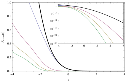
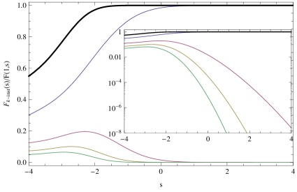
Figure 1: Left: the free energy $F(1,s)$ (black) and its 1- (blue), 2- (red), 3- (yellow), 4-instanton (green) parts.  Right: relative portions $F_{k-{\rm inst}}(s)/F(1,s)$ of $1$- (blue), 2- (red), 3- (yellow), 4-instanton (green) contributions to the free energy, and the sum of these four (black).

4.3 Beyond the strong coupling region

Our identification of the matrix model with the two-dimensional IIA superstrings (4) is limited to the region $s>0$ by construction, as $s<0$ would formally correspond to a negative Liouville coupling $\omega$ or imaginary string coupling $g_{s}$. Nevertheless, the aforementioned smoothness of the free energy as plotted in Fig. 1 leads us to speculate that the $s<0$ region of the matrix model describes some physical system whose weak coupling limit is realized as the IIA superstring theory. As a possible clue in identifying such a system, below we exhibit the asymptotic form of the free energy (at $\xi=1$) in the limit $s\equiv-z\to-\infty$. To this end, we substitute into the Painlevé II equation a formal trans-series ansatz containing a single parameter $C$ [34]:

$$q(z;C)=\sum_{\ell\geq 0}C^{\ell}q_{\ell}(z),\ \ q_{\ell}(z)\sim\frac{e^{-\ell\frac{2\sqrt{2}}{3}z^{3/2}}}{z^{(3\ell-2)/4}}\sum_{n=0}^{\infty}\frac{b_{n}^{(\ell)}}{z^{3n/2}}\ \ (z\to\infty)$$ (53)

with $q_{0}(z)\sim\sqrt{z/2}+\cdots$, and $b_{0}^{(1)}=2^{-1/4}$ by definition. By equating like terms as in section 4.2, the ‘perturbative part’ $q_{0}(z)$ is given by [13]

$$q_{0}(z)\sim\sqrt{\frac{z}{2}}\left(1-\frac{1}{2^{3}z^{3}}-\frac{73}{2^{7}z^{6}}-\frac{10657}{2^{10}z^{9}}+\cdots\right),$$ (54)

and the ‘nonperturbative parts’ $q_{\ell}(z)\ (\ell\geq 1)$ are [34]

$$q_{1}(z) \sim \frac{e^{-\frac{2\sqrt{2}}{3}z^{3/2}}}{2^{1/4}z^{1/4}}\left(1-\frac{17}{2^{9/2}3z^{3/2}}+\frac{1513}{2^{10}3^{2}z^{3}}-\frac{850193}{2^{29/2}3^{4}z^{9/2}}+\cdots\right),$$

$$q_{2}(z) \sim \frac{e^{-\frac{4\sqrt{2}}{3}z^{3/2}}}{2z}\left(1-\frac{41}{2^{7/2}3z^{3/2}}+\frac{5461}{2^{8}3^{2}z^{3}}-\frac{1734407}{2^{23/2}3^{4}z^{9/2}}+\cdots\right),$$

$$q_{3}(z) \sim \frac{e^{-2\sqrt{2}z^{3/2}}}{2^{7/4}z^{7/4}}\left(1-\frac{47}{2^{9/2}z^{3/2}}+\frac{5285}{2^{10}z^{3}}-\frac{1193755}{2^{29/2}3z^{9/2}}+\cdots\right),$$

$$q_{4}(z) \sim \frac{e^{-\frac{8\sqrt{2}}{3}z^{3/2}}}{2^{5/2}z^{5/2}}\left(1-\frac{25}{2^{3/2}3z^{3/2}}+\frac{5011}{2^{6}3^{2}z^{3}}-\frac{1808341}{2^{19/2}3^{4}z^{9/2}}+\cdots\right),$$

$$\cdots$$ . (55)

Since the positive $z$-axis (i.e. negative $s$-axis) is a Stokes line of the Painlevé II equation, one must perform lateral Borel resummations of the formal series (53) by avoiding singularities from above or below, which is denoted by $q_{\pm}(z;C)$. Then the Hastings-McLeod solution is known to be expressed as a median resummation at $C=0$ [34],

$$q_{\rm HM}(-z)=q_{\pm}(z;\mp S/2)=\Re{\rm e}\left[q_{0,\pm}(z)-\frac{1}{4}S^{2}q_{2,\pm}(z)+\frac{5}{16}S^{4}q_{4,\pm}(z)+\cdots\right].$$ (56)

Here $S=-{i}/{\sqrt{2\pi}}$ is the Stokes constant computed in [28, 47], and both of the branches give the same result. Substituting (54), (55) and integrating $q_{\rm HM}(-z)^{2}$ twice in $z$, one finally obtains the asymptotics of the free energy $F(1,-z)$ for $z\to\infty$:

$$F(1,-z) \sim \frac{z^{3}}{12}+\frac{1}{8}\log z-\frac{1}{24}\log 2-\zeta^{\prime}(-1)-\frac{3}{2^{6}z^{3}}-\frac{63}{2^{8}z^{6}}+\cdots$$ (57)

$$+\frac{e^{-\frac{4\sqrt{2}}{3}z^{3/2}}}{2\pi z^{3/2}}\left(\frac{1}{2^{11/2}}-\frac{71}{2^{9}3z^{3/2}}+\frac{13465}{2^{27/2}3^{2}z^{3}}-\frac{5083145}{2^{17}3^{4}z^{9/2}}+\cdots\right)$$

$$+\left(\frac{e^{-\frac{4\sqrt{2}}{3}z^{3/2}}}{2\pi z^{3/2}}\right)^{2}\left(\frac{3}{2^{10}}-\frac{65}{2^{25/2}z^{3/2}}+\frac{3905}{2^{15}3z^{3}}-\frac{3132385}{2^{39/2}3^{3}z^{9/2}}+\cdots\right)$$

$$+\cdots.$$

The integration constant in the above was first conjectured by Tracy and Widom [13] and later proved true in [48]. Note that the leading (perturbative) part of the asymptotics is an expansion in $1/z^{3}$, i.e. each term being proportional to $N^{2-2h}$ with $h\geq 0$, reminiscent of non-supersymmetric closed strings, whereas the nonperturbative parts carrying the instanton action $\frac{4\sqrt{2}}{3}z^{3/2}\propto N$ are expansions in $1/z^{3/2}\propto N^{-1}$, indicating their open string origin.

We have presented asymptotic behavior of the free energy as $s\to\infty$ in section 4.2 and as $s\to-\infty$ here, separately by using trans-series with a single parameter. The instanton effects are different for these regions. For instance, the instanton action in the former (46) is $\frac{4}{3}s^{3/2}$, while that in the latter (57) is $\frac{4\sqrt{2}}{3}(-s)^{3/2}$. It would be interesting to understand the difference from the point of view of resurgence. As discussed in [35], two-parameter trans-series would play a central role in order to perform such a resurgent analysis, which could give an insight into the global structure of the free energy for a complex variable $s$.

5 Condensation of instantons

We have identified ${\rm Det}(1-\hat{K}_{\rm Ai}|_{[s,\infty)})$ with the double-scaled partition function of the SUSY double-well matrix model $Z_{(1,0)}(\mu^{2})$ at $\mu^{2}=2+N^{-2/3}s$. In the grand partition function

$$\Xi(\xi,s)={\rm Det}(1-\xi\hat{K}_{\rm Ai}|_{[s,\infty)}),$$ (58)

$\xi$ can be regarded as fugacity for the matrix model instantons, which should correspond to solitonic objects like D-branes in the two-dimensional IIA superstring theory. Although the instanton fugacity is not explicitly incorporated in the original matrix model with the action (1), it is pleasant surprise that $\xi$ can be naturally introduced into our formulation.

Now that the parameter space of the model is extended to include an instanton chemical potential $\eta=\log\xi$ in addition to the original coupling constant $s$, let us look for a critical line in the $(s,\eta)$-plane. Note that the partition function is a characteristic ‘polynomial’ of the Fredholm eigenvalues $\{\Lambda_{n}(s)\}={\rm Spec}(\hat{K}_{\rm Ai}|_{[s,\infty)})$ as

$$\Xi(e^{\eta},s)=\prod_{n}\left(1-e^{\eta}\Lambda_{n}(s)\right),$$ (59)

where $1\geq\Lambda_{1}(s)>\Lambda_{2}(s)>\cdots\geq 0$ from the argument at the end of section 3, eqs. (33) and (34). If one gradually enhances multi-instanton contributions by turning on a positive chemical potential $\eta>0$ at fixed $s$, the grand partition function vanishes and the corresponding free energy $F(e^{\eta},s)$ diverges logarithmically whenever $e^{-\eta}$ approaches one of the $\Lambda$’s. This property could as well be deduced from the expression of the specific heat (32) in terms of a Painlevé II transcendent $q(s)$. Namely, all of its singularities $\{s_{n}(\eta)\}$ are simple poles that are movable subject to a change of the boundary condition, i.e. the value of $\xi=e^{\eta}$ in (31). This leads to $\partial_{s}^{2}F(e^{\eta},s)=q^{2}\propto(s_{n}(\eta)-s)^{-2}$ and $F(e^{\eta},s)\propto\log(s_{n}(\eta)-s)$ near any one of the singularities in $s$. The critical line accessible from the ‘ordinary’ phase $\eta=0$ is dictated by the largest Fredholm eigenvalue,

$$\eta_{\rm cr}(s)=-\log\Lambda_{1}(s).$$ (60)

We consider that this criticality allows an interpretation as a phase transition due to condensation of instantons, at least for a sufficiently large positive $s$ where the picture of instantons is valid. Subleading eigenvalues $\Lambda_{n\geq 2}(s)$ give a sequence of singularities, but their physical or statistical-mechanical significance is unclear as the grand partition function alternates its sign and becomes negative in the regions $-\log\Lambda_{2n-1}(s)<\eta<-\log\Lambda_{2n}(s)$ ($n=1,2,\cdots$).

As a remark for precise numerical calculation of the spectrum of a trace-class integral operator $\hat{K}|_{I}$, the so-called Nyström-type method (i.e. quadrature approximation) is practically most suited [49]. Namely, after normalizing the interval $I$ to $[-1,1]$ by a linear transformation, one uses the Gauss quadrature method to discretize it into the nodes of the $M$-th order Legendre polynomial $\{x_{i}\}_{i=1}^{M}$ such that $\int_{I}f(x)dx\simeq\sum_{i=1}^{M}f(x_{i})w_{i}$. Here $\{w_{i}\}_{i=1}^{M}$ denotes appropriate positive weights reflecting the density of the nodes. Then the integral operator is discretized into an $M\times M$ real symmetric matrix

$$\hat{K}|_{I}\simeq[K(x_{i},x_{j})\sqrt{w_{i}w_{j}}]_{i,j=1}^{M},$$ (61)

whose eigenvalues can be easily obtained. When applied to the computation of the Fredholm determinant ${\rm Det}(1-\xi\hat{K}|_{I})\simeq\det[\delta_{ij}-\xi K(x_{i},x_{j})\sqrt{w_{i}w_{j}}]_{i,j=1}^{M}$, the discretization error is shown to be suppressed as ${\cal O}(e^{-({\rm const.})\,M})$ [49]. For our purpose of computing the Fredholm eigenvalues and determinant for the Airy kernel (which decreases rapidly for large positive argument(s)) in the range $I=[s,\infty)$ with $|s|\lessapprox 1$, it is sufficient (actually an overkill) to truncate the upper range at $s_{\rm max}=8\sim 10$ and choose $M=100\sim 200$ to achieve double-precision accuracy. In Fig. 2 we exhibit plots of $F(e^{\eta},s)$ and $\eta_{\rm cr}(s)$ computed by this method. It is evident from the plots that for a large positive $s$, the critical value of $\eta$ approaches infinity as

$$\eta_{\rm cr}(s)\sim\frac{4}{3}s^{3/2}+\log(16\pi s^{3/2}),$$ (62)

in consistency with the first two terms of (52). This means that even in the weakly coupled region in $s$, sufficient enhancement of multi-instantons always drives the system to the phase transition of instanton condensation.

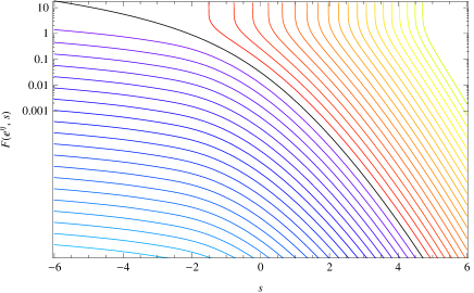
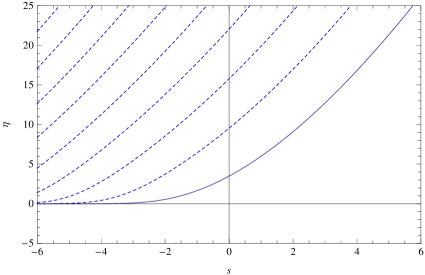
Figure 2: Left: the free energy $F(e^{\eta},s)$ for $\eta=-20,-19,\ldots,-1$ (cyan to purple), $\eta=0$ (black), and $\eta=1,2,\ldots,20$ (red to green). Right: the critical line $\eta=-\log\Lambda_{1}(s)$ (solid curve) in the ($s,\eta$) plane. Subleading Fredholm eigenvalues $-\log\Lambda_{2,3,\cdots}(s)$ are also plotted in broken curves.

6 Discussions

We have identified Tracy and Widom’s cumulative distribution of the largest eigenvalue of GUE as the partition function $Z_{(1,0)}(\mu^{2})$ of the SUSY double-well matrix model describing two-dimensional IIA superstring theory on a nontrivial Ramond-Ramond background. Using this equivalence, strong and weak coupling expansions of the free energy are provided in closed forms by a Painlevé II transcendent. Conceptually, the equivalence leads to a novel observation that the spontaneous breaking of the target-space SUSY in the IIA superstring theory is realized, in terms of the quantum mechanics of the eigenvalues of random matrices, as an exponential tail of the wave function in the classically forbidden domain. By interpreting the spectral parameter $\xi$ in the Fredholm determinant of the Airy kernel as instanton fugacity, we have identified a phase boundary of a transition due to instanton condensation.

Some of future subjects worth examining are listed below:

1. It is interesting to find an S-dual theory which reproduces the strong coupling expansion (37) as a perturbation series. Since this should be called as a noncritical M-theory, it would be helpful to consider a connection with the issue discussed in [50].

2. In this paper, we have focused on the partition function or the free energy of the matrix model. In order to make firmer the correspondence between the matrix model and the two-dimensional IIA superstrings, it is important to proceed computing correlation functions among various matrix-model operators at higher genera and compare the results with the corresponding IIA string amplitudes. For nonperturbative computation beyond the planar level in the matrix model, techniques discussed in [29, 51, 52, 53, 54] would be useful.

3. We have found the equivalence of the free energy of the SUSY matrix model to that of the unitary one-matrix model describing the one-dimensional type 0 string theories in the double scaling limit. It is interesting to investigate whether the equivalence persists for quantities other than the free energy. To this aim, calculation techniques in random matrix theory would be useful to obtain correlation functions of various operators in both sides, similarly to the previous subject.

4. From the viewpoint of random matrix theory, we list three possible extensions of our results:

   • We have dealt with the unitary ($\beta=2$) ensemble whose matrix variables are complex hermitian. For the cases of orthogonal and symplectic ($\beta=1,4$) ensembles in which matrix variables are real symmetric and quaternion selfdual respectively, counterparts of the results presented in section 3 have been obtained [55, 56, 57]. It could be of potential interest to make their interpretations in the string theory side, possibly in a relation to non-orientable worldsheets.

   • The result in section 3 can be generalized such that the Painlevé II equation (30) contains a parameter $\alpha$ [58]:

     $$q^{\prime\prime}(s)=s\,q(s)+2q(s)^{3}+\alpha.$$ (63)

     It reduces to our case in the limit $\alpha\to 0$. According to [53, 59], turning on the parameter $\alpha$ corresponds to introducing ‘quarks’ in the matrix models. While such quarks generate boundaries in a random surface, our interpretation of the matrix model as the IIA superstring theory is not based on the random surface picture. It is intriguing to pursue what kind of deformations of our matrix model amounts to giving (63) and to find its meaning in the string theory side.

   • Multi-critical analogues of the Tracy-Widom distribution for $\beta=2$ was studied in [60, 61, 62] and its interpretation as instanton effects in minimal string theory was presented in [63]. It would be interesting to introduce instanton fugacity for such cases and discuss instanton condensation as in section 5.

5. Alday, Gaiotto and Tachikawa (AGT) [64] found correspondence between instanton sums of four-dimensional ${\cal N}=2$ SUSY gauge theories (the so-called Nekrasov partition functions) [65, 66] and conformal blocks in two-dimensional Liouville field theory. Furthermore, ref. [67] points out that the $\tau$-functions for Painlevé III, V and VI (corresponding to the Fredholm determinants of e.g. Bessel, sine and Hermite kernels, respectively) are all related to $c=1$ conformal blocks, and thus further correspondence is made between the instanton sums of ${\cal N}=2$ SUSY gauge theories with $N_{f}=0,\cdots,4$ and the $\tau$-functions of the Painlevé systems. Since we have found the correspondence of the instanton sum of the two-dimensional IIA superstring theory to the $\tau$-function for Painlevé II (corresponding to the Fredholm determinant of Airy kernel), they are expected to have an analogous relation to some conformal blocks. In addition, existence of the six-dimensional (2,0) theory has been argued to lie behind the AGT correspondence. Likewise, the similarity in our case will lead to existence of the three-dimensional noncritical M-theory mentioned in the first subject.

Appendix A Derivation of (29)-(31)

In this appendix, we present some technical steps relevant to the derivation of (29)-(31). First, the action of a generic integration operator $\hat{O}$ to a function $f(x)$ on $\mathbb{R}$ is expressed by its kernel $O(x,{y})$ as

$$\left(\hat{O}f\right)(x)=\int_{\mathbb{R}}d{y}\,O(x,{y})f({y})\qquad\mbox{and}\qquad\left(f\hat{O}\right)({y})=\int_{\mathbb{R}}dx\,f(x)\,O(x,{y}).$$ (64)

Note that for the kernel $K(x,{y})\chi_{I}({y})$ of the operator $\hat{K}|_{I}$,

$$\left(\hat{K}|_{I}f\right)(x) = \int_{\mathbb{R}}d{y}\,K(x,{y})\chi_{I}({y})f({y})=\int_{I}d{y}\,K(x,{y})f({y}),$$

$$\left(f\hat{K}|_{I}\right)({y}) = \int_{\mathbb{R}}dx\,f(x)\,K(x,{y})\chi_{I}({y}).$$ (65)

Suppose $K(x,{y})$ takes the form:

$$K(x,{y})=\frac{A(x)B({y})-B(x)A({y})}{x-{y}}.$$ (66)

For the position operator $\hat{x}$ specified by its kernel $x\,\delta(x-{y})$, the kernel of $[\hat{x},(1-\hat{K}|_{I})^{-1}]$ is given by 

$$(x-{y})\rho(x,{y})=(Q(x)\,P({y})-P(x)\,Q({y}))\,\chi_{I}({y})$$ (67)

with $\rho(x,{y})$ being the kernel of $(1-\hat{K}|_{I})^{-1}$ and

$$Q(x) := \left((1-\hat{K}|_{I})^{-1}A\right)(x)=\int_{\mathbb{R}}d{y}\,\rho(x,{y})\,A({y}),$$

$$P(x) := \left((1-\hat{K}|_{I})^{-1}B\right)(x)=\int_{\mathbb{R}}d{y}\,\rho(x,{y})\,B({y}).$$ (68)

From the expansion $(1-\hat{K}|_{I})^{-1}=1+\sum_{n=1}^{\infty}(\hat{K}|_{I})^{n}$, we can see that $\rho(x,y)=0$ for $x\in I$ and $y\notin I$. For the resolvent operator

$$\hat{R}:=(1-\hat{K}|_{I})^{-1}\hat{K}|_{I}=(1-\hat{K}|_{I})^{-1}-1,$$ (69)

its kernel $K(x,{y})$ takes the form

$$R(x,y)=\,\frac{Q(x)\,P(y)-P(x)\,Q({y})}{x-y}\,\chi_{I}(y)$$ (70)

since the kernel of $[\hat{x},\hat{R}]$ is nothing but (67). The definition indicates that the diagonal part of the kernel is given by the logarithmic derivative of the Fredholm determinant:

$$R(a,a)=\frac{d}{da}\,\log\mbox{Det}(1-\hat{K}|_{I}).$$ (71)

Hereafter we consider the interval $I=[a,\infty)$ ($a$ will be eventually set to $2+N^{-2/3}s$).

A.1 JMMS equations

In the case of the Hermite kernel of GUE, $A(x)$ and $B(x)$ can be identified with the wave functions: $A(x)=\sqrt{\xi}\,\psi_{N}(x)$ and $B(x)=\sqrt{\xi}\,\psi_{N-1}(x)$. Hence they satisfy

$$\frac{d}{dx}\begin{pmatrix}A(x)\\ B(x)\end{pmatrix}=N\begin{pmatrix}-\frac{1}{2}x&1\\ -1&\frac{1}{2}x\end{pmatrix}\begin{pmatrix}A(x)\\ B(x)\end{pmatrix}.$$ (72)

For the derivative operator $\hat{d}$ associated with the kernel $\delta^{\prime}(x-y)$, the kernel of $[\hat{d},(1-\hat{K}|_{I})^{-1}]$ is obtained as

$$-\frac{N}{2}\,(Q(x)\,P(y)+P(x)\,Q(y))\,\chi_{I}(y)+R(x,a)\,\rho(a,y).$$ (73)

Use of (68), (72) and (73) leads to

$$\frac{d}{dx}Q(x) = -\frac{N}{2}x\,Q(x)+N(1-u)\,P(x)+R(x,a)\,q,$$

$$\frac{d}{dx}P(x) = \frac{N}{2}x\,P(x)-N(1+w)\,Q(x)+R(x,a)\,p,$$ (74)

where $u=\int_{I}dx\,Q(x)\,A(x)$, $w=\int_{I}dx\,P(x)\,B(x)$, $q=Q(a)$ and $p=P(a)$. Here and in what follows, quantities at the boundary $x=a$ are defined by taking the limit $x\to a+0$, i.e. the limit from the inside of $I$. Also,

$$\frac{\partial}{\partial a}Q(x)=-R(x,a)\,q,\qquad\frac{\partial}{\partial a}P(x)=-R(x,a)\,p$$ (75)

are derived from the fact that the kernel of $\frac{\partial}{\partial a}(1-\hat{K}|_{I})^{-1}$ is $-R(x,a)\,\rho(a,y)$. Together with this, (74) gives

$$\frac{dq}{da} = \left.\left(\frac{d}{dx}+\frac{\partial}{\partial a}\right)Q(x)\right|_{x=a}=-\frac{N}{2}a\,q+N(1-u)\,p,$$

$$\frac{dp}{da} = \left.\left(\frac{d}{dx}+\frac{\partial}{\partial a}\right)P(x)\right|_{x=a}=\frac{N}{2}a\,p-N(1+w)\,q$$ (76)

and

$$\frac{\partial u}{\partial a}=-q^{2},\qquad\frac{\partial w}{\partial a}=-p^{2}.$$ (77)

Finally, (70) at $x=y=a$ is expressed as

$$R(a,a) = \left.\left[\Bigl{(}\frac{d}{dx}Q(x)\Bigr{)}\,P(x)-\Bigl{(}\frac{d}{dx}P(x)\Bigr{)}\,Q(x)\right]\right|_{x=a}$$ (78)

$$= N\left[-a\,p\,q+(1-u)\,p^{2}+(1+w)\,q^{2}\right].$$

(76), (77) and (78) are the Jimbo-Miwa-Môri-Sato (JMMS) equations [68] for the half-infinite interval $I$, from which we shall obtain a closed differential equation for the diagonal resolvent.

A.2 Painlevé VI equation for the diagonal resolvent

From the JMMS equations, we find

$$\frac{d}{da}R(a,a) = -N\,p\,q,$$ (79)

$$\frac{d}{da}(p\,q) = N(1-u)\,p^{2}-N(1+w)\,q^{2},$$ (80)

$$\frac{d}{da}(u-w+uw) = (1-u)\,p^{2}-(1+w)\,q^{2}.$$ (81)

The last two equations mean that $p\,q$ is equal to $N(u-w+uw)$ up to an additive $a$-independent constant. However, the fact that all of $p$, $q$, $u$ and $w$ vanish as $a\to\infty$ determines the constant to be nil. Namely,

$$p\,q=N(u-w+uw).$$ (82)

With the help of (79), (80) and the JMMS equations, we have

$$\frac{d^{3}}{da^{3}}R(a,a)=-N\,\frac{d}{da}\left[2Np^{2}q^{2}+N\,a\{R(a,a)+Na\,p\,q\}-4N^{2}(1-u)(1+w)\,p\,q\right].$$ (83)

After the use of (79) following (82), we finally obtain a differential equation for $R(a,a)$:

$$\frac{d^{3}}{da^{3}}R(a,a)=-N^{2}a\,R(a,a)+N^{2}(a^{2}-4)\,\frac{d}{da}R(a,a)-6\Bigl{(}\frac{d}{da}R(a,a)\Bigr{)}^{2},$$ (84)

which can be transformed to Okamoto’s $\sigma$-form [69] of a Painlevé VI equation.

A.3 Soft edge scaling limit and Painlevé II equation

In the soft edge scaling limit $a=2+N^{-2/3}s$, (26) indicates that the diagonal resolvent scales as $R(a,a)=N^{2/3}R(s)$. Then, (84) becomes

$$R^{\prime\prime\prime}(s)=-2R(s)+4s\,R^{\prime}(s)-6R^{\prime}(s)^{2}.$$ (85)

Integration of (85) after multiplied by $R^{\prime\prime}(s)$ leads to

$$\frac{1}{4}\,R^{\prime\prime}(s)^{2}=-R(s)\,R^{\prime}(s)+s\,R^{\prime}(s)^{2}-R^{\prime}(s)^{3}.$$ (86)

Exponential decay of $R(s)$ as $s\to\infty$ is clear from the behavior of the Airy kernel (26). We used it as an initial condition of the integration. Setting $R(s)=\int_{s}^{\infty}dt\,q(t)^{2}$, we see that the Painlevé II equation (30) is obtained from (86). Accordingly, the scaling limit of (71) with $\xi$ restored takes the form

$$\frac{d}{ds}\log\mbox{Det}(1-\xi\hat{K}_{\rm Ai}|_{[s,\infty)})=R(s)=\int_{s}^{\infty}dt\,q(t)^{2}.$$ (87)

For $\xi$ small, differentiating (87) with respect to $s$ gives

$$q(s)^{2}=\xi\frac{d}{ds}K_{\rm Ai}(s,s)+{\cal O}(\xi^{2})=\xi{\rm Ai}(s)^{2}+{\cal O}(\xi^{2})$$ (88)

with use of (26). This yields the boundary condition (31), since the ${\cal O}(\xi^{2})$ terms consist of higher powers of the Airy function and become negligible as $s\to\infty$. Finally, (29) follows from (87), where the integration constant is fixed by the small-$\xi$ behavior.

References

- [1] T. Banks, W. Fischler, S. H. Shenker and L. Susskind, Phys. Rev. D 55 (1997) 5112 [arXiv:hep-th/9610043].
- [2] N. Ishibashi, H. Kawai, Y. Kitazawa and A. Tsuchiya, Nucl. Phys. B 498 (1997) 467 [arXiv:hep-th/9612115].
- [3] L. Motl, arXiv:hep-th/9701025.
- [4] R. Dijkgraaf, E. P. Verlinde and H. L. Verlinde, Nucl. Phys. B 500 (1997) 43 [arXiv:hep-th/9703030].
- [5] J. M. Maldacena, Adv. Theor. Math. Phys. 2 (1998) 231; [Int. J. Theor. Phys. 38 (1999) 1113] [arXiv:hep-th/9711200].
- [6] N. Itzhaki, J. M. Maldacena, J. Sonnenschein and S. Yankielowicz, Phys. Rev. D 58 (1998) 046004 [arXiv:hep-th/9802042].
- [7] T. Kuroki and F. Sugino, Nucl. Phys. B 830 (2010) 434 [arXiv:0909.3952 [hep-th]].
- [8] T. Kuroki and F. Sugino, Nucl. Phys. B 844 (2011) 409 [arXiv:1009.6097 [hep-th]].
- [9] H. Ita, H. Nieder and Y. Oz, JHEP 0506 (2005) 055 [hep-th/0502187].
- [10] T. Kuroki and F. Sugino, Nucl. Phys. B 867 (2013) 448 [arXiv:1208.3263 [hep-th]].
- [11] T. Kuroki and F. Sugino, JHEP 1403 (2014) 006 [arXiv:1306.3561 [hep-th]].
- [12] M. G. Endres, T. Kuroki, F. Sugino and H. Suzuki, Nucl. Phys. B 876 (2013) 758 [arXiv:1308.3306 [hep-th]].
- [13] C. A. Tracy and H. Widom, Commun. Math. Phys. 159 (1994) 151 [hep-th/9211141].
- [14] C. A. Tracy and H. Widom, Commun. Math. Phys. 163 (1994) 33 [hep-th/9306042].
- [15] C. A. Tracy and H. Widom, in: Proceedings of the ICM. Vol. 1, pp. 587–596 (Beijing, 2002) [math-ph/0210034].
- [16] P. J. Forrester and N. S. Witte, arXiv:1210.3381 [math-ph].
- [17] S. N. Majumdar and G. Schehr, J. Stat. Mech. (2014) P01012 [arXiv:1311.0580 [cond-mat]].
- [18] J. Baik, P. Deift and K. Johansson, J. Amer. Math. Soc. 12 (1999) 1119 [math.CO/9810105].
- [19] K. Johansson, Commun. Math. Phys. 209 (2000) 437 [math/9903134 [math.CO]].
- [20] C. A. Tracy, and H. Widom, Commun. Math. Phys. 290 (2009) 129 [arXiv:0807.1713 [math.PR]].
- [21] M. Prähofer and H. Spohn, Phys. Rev. Lett. 84 (2000) 4882 [cond-mat/9912264].
- [22] K. A. Takeuchi, M. Sano, T. Sasamoto and H. Spohn, Sci. Rep. 1 (2011) 34 [arXiv:1108.2118 [cond-mat]].
- [23] I. Corwin, Random Matrices: Theory Appl. 1 (2012) 1130001 [arXiv:1106.1596 [math.PR]].
- [24] V. Periwal and D. Shevitz, Phys. Rev. Lett. 64 (1990) 1326; Nucl. Phys. B 344 (1990) 731.
- [25] G. Szegő, “Orthogonal Polynomials,” 4th ed., American Mathematical Society (Providence, 1975).
- [26] P. J. Forrester and N. S. Witte, Commun. Math. Phys. 219 (2001) 357 [math-ph/0103025].
- [27] S. P. Hastings and J. B. McLeod, Arch. Rat. Mech. Anal. 73 (1980) 31.
- [28] A. S. Fokas, A. R. Its, A. A. Kapaev and V. Y. Novokshenov, “Painlevé Transcendents: The Riemann-Hilbert Approach”, American Mathematical Society (Providence, 2006).
- [29] I. R. Klebanov, J. M. Maldacena and N. Seiberg, Commun. Math. Phys. 252 (2004) 275 [hep-th/0309168].
- [30] D. J. Gross and E. Witten, Phys. Rev. D 21 (1980) 446.
- [31] S. R. Wadia, Phys. Lett. B 93 (1980) 403.
- [32] D. J. Gross and A. Matytsin, Nucl. Phys. B 429 (1994) 50 [hep-th/9404004].
- [33] P. J. Forrester, S. N. Majumdar, G. Schehr, Nucl. Phys. B 844 (2011) 500 [Erratum ibid. B857 (2012) 424] [arXiv:1009.2362 [math-ph]].
- [34] M. Mariño, JHEP 0812 (2008) 114 [arXiv:0805.3033 [hep-th]].
- [35] R. Schiappa and R. Vaz, Commun. Math. Phys. 330 (2014) 655 [arXiv:1302.5138 [hep-th]].
- [36] M. Mariño, R. Schiappa and M. Weiss, Commun. Num. Theor. Phys. 2 (2008) 349 [arXiv:0711.1954 [hep-th]]; J. Math. Phys. 50 (2009) 052301 [arXiv:0809.2619 [hep-th]].
- [37] S. Pasquetti and R. Schiappa, Annales Henri Poincaré 11 (2010) 351 [arXiv:0907.4082 [hep-th]].
- [38] I. Aniceto, R. Schiappa and M. Vonk, Commun. Num. Theor. Phys. 6 (2012) 339 [arXiv:1106.5922 [hep-th]].
- [39] G. V. Dunne and M. Ünsal, JHEP 1211 (2012) 170 [arXiv:1210.2423 [hep-th]]; Phys. Rev. D 89 (2014) 041701 [arXiv:1306.4405 [hep-th]].
- [40] G. Basar, G. V. Dunne and M. Ünsal, JHEP 10 (2013) 041 [arXiv:1308.1108 [hep-th]].
- [41] A. Cherman, D. Dorigoni and M. Ünsal, arXiv:1403.1277 [hep-th].
- [42] E. Witten, Nucl. Phys. B 202 (1982) 253.
- [43] F. Olver, “Asymptotics and Special Functions”, Academic Press (London, 1974).
- [44] N. S. Witte, F. Bornemann and P. J. Forrester, Nonlinearity 26 (2013) 1799 [arXiv:1209.2190 [math.CA]].
- [45] M. Prähofer and H. Spohn, J. Stat. Phys. 115 (2004) 255 [cond-mat/0212519].
- [46] P. J. Forrester, “Log-Gases and Random Matrices”, Princeton Univ. Press (Princeton, 2010).
- [47] H. Kawai, T. Kuroki and Y. Matsuo, Nucl. Phys. B 711 (2005) 253 [hep-th/0412004].
- [48] P. Deift, A. Its and I. Krasovsky, Commun. Math. Phys. 278 (2008) 643 [math/0609451].
- [49] F. Bornemann, Math. Comp. 79 (2010) 871 [arXiv:0804.2543 [math.NA]]; Markov Processes Relat. Fields 16 (2010) 803 [arXiv:0904.1581 [math.PR]].
- [50] P. Hořava and C. A. Keeler, JHEP 0707 (2007) 059 [hep-th/0508024].
- [51] Č. Crnković and G. W. Moore, Phys. Lett. B 257 (1991) 322.
- [52] S. Dalley, C. V. Johnson and T. Morris, Nucl. Phys. B 368 (1992) 625.
- [53] G. Akemann, P. H. Damgaard, U. Magnea and S. M. Nishigaki, Nucl. Phys. B 519 (1998) 682 [hep-th/9712006].
- [54] T. Claeys and A. B. J. Kuijlaars, Comm. Pure Appl. Math. 59 (2006) 1573 [math-ph/0501074].
- [55] C. A. Tracy and H. Widom, Commun. Math. Phys. 177 (1996) 727 [solv-int/9509007].
- [56] P. J. Forrester and E. M. Rains, in: (Ed.) P. M. Bleher and A. R. Its, “Random matrix models and their applications,” vol. 40 of Mathematical Sciences Research Institute Publications, pp. 171–208, Cambridge Univ. Press (Cambridge, 2001) [solv-int/9907008].
- [57] P. Desrosiers and P. J. Forrester, Nonlinearity 19 (2006) 1643 [math-ph/0604027].
- [58] T. Claeys, A. B. J. Kuijlaars and M. Vanlessen, Ann. Math. 168 (2008) 601 [math-ph/0508062].
- [59] J. A. Minahan, Phys. Lett. B 268 (1991) 29.
- [60] T. Claeys, A. Its and I. Krasovsky, Comm. Pure Appl. Math. 63 (2010) 362 [arXiv:0901.2473 [math-ph]].
- [61] T. Claeys and S. Olver, in: (Ed.) J. Arvesú and G. López Lagomasino, “Contemporary Mathematics: Recent Advances in Orthogonal Polynomials, Special Functions, and Their Applications”, pp. 83–98, American Mathematical Society (Providence, 2012) [arXiv:1111.3527 [math-ph]].
- [62] G. Akemann and M. R. Atkin, J. Phys. A 46 (2013) 015202 [arXiv:1208.3645 [math-ph]].
- [63] M. R. Atkin and S. Zohren, JHEP 1404 (2014) 118 [arXiv:1307.3118 [math-ph]].
- [64] L. F. Alday, D. Gaiotto and Y. Tachikawa, Lett. Math. Phys. 91 (2010) 167 [arXiv:0906.3219 [hep-th]].
- [65] N. A. Nekrasov, Adv. Theor. Math. Phys. 7 (2004) 831 [hep-th/0206161].
- [66] N. A. Nekrasov and A. Okounkov, hep-th/0306238.
- [67] O. Gamayun, N. Iorgov and O. Lisovyy, J. Phys. A 46 (2013) 335203 [arXiv:1302.1832 [hep-th]].
- [68] M. Jimbo, T. Miwa, Y. Môri and M. Sato, Physica D 1 (1980) 80.
- [69] K. Okamoto, Ann. Mat. Pura Appl. 146 (1987) 337.
- [70]