Topological surface states and Andreev bound states in superconducting iron pnictides

Abstract

The nontrivial topology of the electronic structure of iron pnictides can lead to the appearance of surface states. We study such states in various strip geometries with a focus on the superconducting phase. In the presence of unconventional superconducting pairing with $s_{\pm}$-wave gap structure, the topological states are quite robust and partly remain in the superconducting gap. Furthermore, Andreev bound states appear, which coexist with the topological states for small superconducting gaps and merge with them for larger gap values. The bulk and surface dispersions are obtained from exact diagonalization for two-orbital and five-orbital models in strip geometries.

I Introduction

In the past few years, the iron pnictidesJoh10 ; DHD12 on the one hand and topological properties of matterHaK10 ; QiZ11 on the other have been two of the most active fields in condensed-matter physics. Iron pnictides feature unconventional multiband superconductivity with high transition temperatures competing with itinerant antiferromagnetism. Topology is of particular interest for condensed matter since nontrivial topological properties of the band structure in the bulk are related to the existence of surface or edge states. Previously, we have predicted that iron pnictides in the paramagnetic and antiferromagnetic states can have surface states of topological origin at (100) surfaces.LaT13 Here, we investigate the surface states in the superconducting phase. We focus on the interplay of surface states of topological origin with Andreev bound states enabled by unconventional superconductivity.

The surface states in the paramagnetic phase and in the antiferromagnetic spin-density-wave (SDW) phase result from winding of the momentum-dependent Hamiltonian in orbital space, in particular with respect to the iron $d_{xz}$ and $d_{yz}$ orbitals, noted already by Ran et al.RWZ09 The surface states are of topological origin in the sense that the model Hamiltonian can be deformed, without closing the gap existing in certain ranges of surface momenta, into one that is topologically nontrivial and has flat bands of surface states at the Fermi energy. Reversing the deformation, the topological protection of these surface states is lost, but they evolve continuously as a function of the deformation. Thus the surface bands become dispersive and generally move away from the Fermi energy but are not destroyed until they merge with the continuum of bulk bands.LaT13 The same type of argument can explain the edge states at graphene zigzag edges, which form nearly but not quite flat bands.CGP09 ; KOQ11 Since we are using two-dimensional models, the surface states of slabs emerge as edge states of strips. Using two-dimensional models corresponds to neglecting the dispersion in the $k_{z}$ direction. If we took the $k_{z}$ dispersion of the bulk bands into account, the surface states would survive but also become dispersive.

Many iron pnictides show superconductivity in the vicinity of, or even coexisting with, antiferromagnetism.TBN08 ; LKK09 ; PTK09 ; GAB09 ; LuC10 ; WLP11 ; ACG11 It is therefore of interest how the surface states are modified when a superconducting gap opens. The superconducting order parameter of the 1111 family of iron pnictides is thought to be of $s_{\pm}$-wave form, i.e., it has opposite sign on the electron-like and the hole-like Fermi pockets.HKM11 ; Chu12 The gap does not have nodes on the Fermi surface. Andreev bound states have been studied for a simple two-band model by Onari and TanakaOnT09 and, within a quasiclassical approximation, by Nagai et al.NaH09 The latter group has extended their study to a five-orbital model.NHM10 Huang and LinHuL10 consider Anreev bound states for a two-orbital model. We here find Andreev bound states inside the superconducting gap that coexist with the topological surface states for small gap magnitudes and merge with them at larger gap values. We also present additional results for the paramagnetic and SDW phases, for strip orientations not considered in Ref. LaT13, . We will employ a simple two-orbital model and a more realistic five-orbital model.LaT13 ; RWZ09 ; KOA08

The remainder of this paper is organized as follows. In Sec. II, we introduce the two-orbital and five-orbital models used in our study. We then discuss the mean-field approximations for the SDW and superconducting phases and the exact diagonalization for strip geometries. In Sec. III, we present numerical results for the dispersion of strips in the superconducting state, compare them to the paramagnetic and antiferromagnetic states, and discuss the origin of the different types of surface states. In Sec. IV we summarize the results and draw conclusions.

II Models and method

The two-orbital model of Ran et al.RWZ09 is formulated for a two-dimensional iron square lattice and involves only the $3d_{XZ}$ and $3d_{YZ}$ orbitals in a single-iron unit cell. The $X$ and $Y$ axes are rotated by $45^{\circ}$ relative to the $x$ and $y$ axes of the lattice. The noninteracting Hamiltonian used to model the paramagnetic phase reads $H_{0}=\sum_{\mathbf{k}\sigma}\sum_{a,b=1}^{2}\mathcal{H}_{ab}^{0}(\mathbf{k})\,d_{\mathbf{k}a\sigma}^{\dagger}d_{\mathbf{k}b\sigma}$ with the $2\times 2$ matrixRWZ09

$$\mathcal{H}^{0}(\mathbf{k})=2t_{1}(\cos k_{x}-\cos k_{y})\,\tau^{1}$$ (1)

$${}-2(t_{2}-t_{2}^{\prime})\sin k_{x}\sin k_{y}\,\tau^{3}$$

$${}+[2(t_{2}+t_{2}^{\prime})\cos k_{x}\cos k_{y}+2t_{1}^{\prime}(\cos k_{x}+\cos k_{y})]\,\tau^{0}\quad$$

in orbital space. Here, $\tau^{1}$, $\tau^{2}$, $\tau^{3}$ are Pauli matrices, $\tau^{0}$ is the unit matrix, the index $1$ corresponds to $3d_{XZ}$, and the index $2$ to $3d_{YZ}$. The hopping parameters are chosen to be $t_{1}=0.30\,\mathrm{eV}$, $t_{1}^{\prime}=0.06\,\mathrm{eV}$, $t_{2}=0.51\,\mathrm{eV}$, and $t_{2}^{\prime}=0.09\,\mathrm{eV}$.RWZ09 Note that the band structure of this model features quadratic band touching points in the center and at the corners of the Brillouin zone (BZ).

In order to model the antiferromagnetic phase, we use the interacting Hamiltonian $H=H_{0}+H_{I}$ withRWZ09

$$H_{I} = \frac{U}{2}\sum_{\mathbf{j}}(\hat{n}_{\mathbf{j}1}^{2}+\hat{n}_{\mathbf{j}2}^{2})+(U-2J)\sum_{\mathbf{j}}\hat{n}_{\mathbf{j}1}\,\hat{n}_{\mathbf{j}2}$$ (2)

$${}+J\sum_{\mathbf{j}}\sum_{\sigma\sigma^{\prime}}d_{\mathbf{j}1\sigma}^{\dagger}d_{\mathbf{j}2\sigma^{\prime}}^{\dagger}d_{\mathbf{j}1\sigma^{\prime}}d_{\mathbf{j}2\sigma}$$

$${}+J\sum_{\mathbf{j}}(d_{\mathbf{j}1\uparrow}^{\dagger}d_{\mathbf{j}1\downarrow}^{\dagger}d_{\mathbf{j}2\downarrow}d_{\mathbf{j}2\uparrow}+\textrm{H.c.}),$$

where $\hat{n}_{\mathbf{j}a}\equiv\sum_{\sigma}d_{\mathbf{j}a\sigma}^{\dagger}d_{\mathbf{j}a\sigma}$. For the interaction parameters, we take $U=1.20\,\textrm{eV}$ and $J=0.12\,\textrm{eV}$. RWZ09 A mean-field decoupling of the form LaT13 $\langle d_{\mathbf{j}a\sigma}^{\dagger}d_{\mathbf{j}b\sigma}\rangle=n_{ab}+\frac{\sigma}{2}\,(-1)^{j_{x}}\,m_{ab}$, where we have assumed an SDW ordering vector $\mathbf{Q}=(\pi,0)$ and spins pointing along the $S_{z}$ axis, then leads to the mean-field Hamiltonian

$$H_{\mathrm{MF}}=H_{0}+\sum_{\mathbf{j}}\sum_{a,b}(-1)^{j_{x}}M_{ab}\,(d_{\mathbf{j}a\uparrow}^{\dagger}d_{\mathbf{j}b\uparrow}-d_{\mathbf{j}a\downarrow}^{\dagger}d_{\mathbf{j}b\downarrow}),$$ (3)

with $M_{11}=-(Um_{11}+Jm_{22})/2$, $M_{22}=-(Um_{22}+Jm_{11})/2$, and $M_{12}=M_{21}=-Jm_{12}=-Jm_{21}$.LaT13 The mean-field coefficients $m_{ab}$ are calculated self-consistently assuming half filling.

For the superconducting phase, we employ the BCS mean-field Hamiltonian

$$H_{\mathrm{BCS}}=\sum_{\mathbf{k}\sigma}\sum_{ab}[\mathcal{H}^{0}_{ab}(\mathbf{k})-\delta_{ab}\mu]\,d_{\mathbf{k}a\sigma}^{\dagger}d_{\mathbf{k}b\sigma}$$ (4)

$${}-\sum_{\mathbf{k}}\sum_{ab}\big{[}\Delta_{ab}(\mathbf{k})\,d_{\mathbf{k}a\uparrow}^{\dagger}d_{-\mathbf{k},b,\downarrow}^{\dagger}+\Delta_{ab}^{*}(\mathbf{k})\,d_{-\mathbf{k},b,\downarrow}d_{\mathbf{k}a\uparrow}\big{]},\quad$$

where $\mu$ denotes the chemical potential at half filling. For the superconducting gap function we use $\Delta_{ab}(\mathbf{k})=\Delta\,\delta_{ab}$ for conventional $s_{++}$-wave pairing and $\Delta_{ab}(\mathbf{k})=\Delta\,\delta_{ab}\,\cos k_{x}\cos k_{y}$ for the unconventional $s_{\pm}$-wave pairing likely realized in 1111 iron pnictides.HKM11 ; Chu12 The sign structure of the gap function with $s_{\pm}$-wave gap structure is illustrated in Fig. 1 along with typical Fermi surfaces for the two-orbital and five-orbital models. Note that there is a sign change of the superconducting gap between electron and hole Fermi pockets. The corresponding Bogoliubov-de Gennes (BdG) Hamiltonian for our model is a $4\times 4$ matrix, which readsHuL10

$$\mathcal{H}_{\mathrm{BdG}}=\begin{pmatrix}\mathcal{H}^{0}(\mathbf{k})-\mu\tau^{0}&-\Delta(\mathbf{k})\\ -\Delta^{\dagger}(\mathbf{k})&-\mathcal{H}^{0}(\mathbf{-k})+\mu\tau^{0}\end{pmatrix}$$ (5)

with respect to the basis $\{d_{\mathbf{k}1\uparrow}^{\dagger},\,d_{\mathbf{k}2\uparrow}^{\dagger},\,d_{-\mathbf{k},1,\downarrow},\,d_{-\mathbf{k},2,\downarrow}\}$. The two-orbital modelRWZ09 used here and in Ref. HuL10, is different from the model employed for the study of Andreev bound states in Refs. OnT09, ; NaH09, . The latter has only one electron and one hole Fermi pocket each and is effectively rotated by $45^{\circ}$ compared to our model.

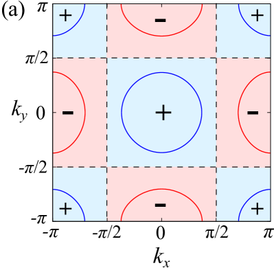
(a)

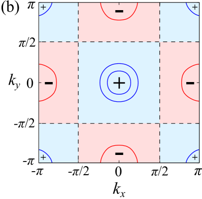
(b)

Figure 1: (Color online) Sign structure of the superconducting gap function with $s_{\pm}$-wave structure. The red (blue) areas denote regions in the BZ where the sign of $\cos k_{x}\cos k_{y}$ is negative (positive). The dashed lines show the nodes of this function. In addition, the Fermi surfaces of (a) the two-orbital model and (b) the five-orbital model are plotted.

The more realistic five-orbital model of Kuroki et al.KOA08 includes all hopping amplitudes larger than $10\,\mathrm{meV}$ up to fifth neighbors. Along with the onsite energies, they are obtained from density-functional calculations for LaFeAsO and are tabulated in Ref. KOA08, . Moreover, the orbital indices now assume values $a,b=1,\ldots,5$ corresponding to $3d_{3Z^{2}-R^{2}}$, $3d_{XZ}$, $3d_{YZ}$, $3d_{X^{2}-Y^{2}}$, $3d_{XY}$, respectively. Note that the band structure of the five-orbital model exhibits, besides quadratic band touching points, also Dirac points.

The interaction Hamiltonian for the antiferromagnetic phase is basically the same as for the two-orbital model, except that the interorbital terms in Eq. (2) now become sums over all pairs of five orbitals. For the interaction parameters we take $U=1.0\,\mathrm{eV}$ and $J=0.2\,\mathrm{eV}$.RWZ09 A decoupling as above then yields a mean-field Hamiltonian analogous to Eq. (3). The corresponding coefficients $M_{ab}$ are given in Ref. LaT13, . The mean-field parameters $m_{ab}$ are calculated self-consistently, assuming $6$ electrons per iron, corresponding to zero doping. The BCS Hamiltonian for the superconducting phase is analogous to the two-orbital case, taking the larger number of orbitals into account.

We are interested in edge states of strips described by the two models. Specifically, we investigate strips of width $W$ with (10), (01), and (11) edges. We assume that the SDW and superconducting strips are described by the same uniform order parameters $m_{ab}$ and $\Delta$ as the bulk systems. We briefly return to this point in Sec. IV.

For a strip with (10) edges, $k_{y}$ is still a good quantum number since the strip is extended along the $y$ axis. Therefore, we carry out a Fourier transformation in the $y$ direction, $d_{\mathbf{j}a}^{\dagger}=N_{y}^{-1/2}\sum_{k_{y}}e^{-ik_{y}j_{y}}\,d_{j_{x}k_{y}a}^{\dagger}$, giving a block-diagonal Hamiltonian with blocks enumerated by $k_{y}$. The dimension of the blocks is a multiple of $W$. The energy bands of the (10) strip are then obtained by exact diagonalization of these blocks. For strips with (01) edges, we simply interchange the roles of $x$ and $y$.

Figure 2: New unit cell and (11) edges: (a) Comparison of the old unit cell (dashed square) and the new unit cell (solid square). The new unit cell is rotated by $45^{\circ}$ and its sides are stretched by a factor of $\sqrt{2}$. $a$ is the lattice constant. (b) Strip with two (11) edges in the rotated coordinate system. Black (grey) dots belong to sublattice $A$ ($B$). The strip width is $W=N_{X}$. The new unit cell is depicted by a solid square.

Strips with (11) edges require a different treatment since the edges cut diagonally through the lattice. It is convenient to use a unit cell with two sides parallel to the (11) edges, see Fig. 2. The new unit cell contains two iron sites. For this reason, we can describe the lattice in terms of two quadratic sublattices $A$ and $B$. We further introduce a new coordinate system, whose axes, denoted by $X$ and $Y$, are rotated by $45^{\circ}$ with respect to the old coordinate system and are thus aligned with the sides of the new unit cell. After representing $H_{0}$, $H_{\mathrm{MF}}$, and $H_{\mathrm{BCS}}$ in the new coordinates, we perform a Fourier transformation in the $Y$ direction,

$$d_{j_{X}j_{Y}aA}^{\dagger} = \frac{1}{\sqrt{N_{Y}}}\sum_{k_{Y}}e^{-i\sqrt{2}\,k_{Y}j_{Y}}\,d_{j_{X}k_{Y}aA}^{\dagger},$$ (6)

$$d_{j_{X}j_{Y}aB}^{\dagger} = \frac{1}{\sqrt{N_{Y}}}\sum_{k_{Y}}e^{-i\frac{k_{Y}}{\sqrt{2}}}\,e^{-i\sqrt{2}\,k_{Y}j_{Y}}\,d_{j_{X}k_{Y}aB}^{\dagger},$$ (7)

where $k_{Y}\in(-\pi/\sqrt{2},\pi/\sqrt{2}]$ and $N_{Y}$ is the number of unit cells along the $Y$ axis. This leads to a block Hamiltonian, which we diagonalize to obtain the energy bands.

III Results and discussion

III.1 Strips with (10) or (01) edges

Paramagnetic and antiferromagnetic phase

Our results for strips with (10) edges in the paramagnetic and in the antiferromagnetic phase, obtained in Ref. LaT13, , are briefly summarized in the following. In the two-orbital model, four bands of edge states are present in the paramagnetic phase. They are exactly degenerate in pairs due to SU(2) spin-rotation symmetry. The two pairs are bonding and anti-bonding combinations of states localized at the two edges and become degenerate in the limit of a broad strip. In the five-orbital model, two such groups of four nearly degenerate bands appear. As noted in the introduction, the existence of surface states can be understood from an argument based on a continuous deformation, which does not close the gap, of the Hamiltonian into a topologically nontrivial one. Upon turning on SDW order with ordering vector $\mathbf{Q}=(\pi,0)$, the asymptotically degenerate bundles of bands split due to the coupling of the spin of the electrons localized at the surface to the SDW order parameter, which is uniform along the (10) edges. However, they remain exactly degenerate in pairs since the corresponding mean-field Hamiltonian is still invariant under combined spin rotation by $\pi$ about the $x$ axis and spatial reflection $x\rightarrow-x$.

For the antiferromagnetic phase with ordering vector $(\pi,0)$, the (01) edge is not equivalent to the (10) edge. For the (01) edge, the magnetic unit cell is doubled in the $x$ direction and thus the one-dimensional (1D) edge BZ is halved. As a consequence, the number of surface bands doubles, due to the folding of the spectrum, and the resulting degeneracy at the boundaries of the magnetic BZ is lifted by the SDW. Unlike for the (10) edge, the original four-fold degeneracy of the surface bands for $W\to\infty$ remains intact (not shown). This is because the magnetization at the (01) edges is staggered so that states of opposite spin localized at the same edge are not split. These observations hold for both models.

Superconducting phase

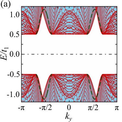
(a)

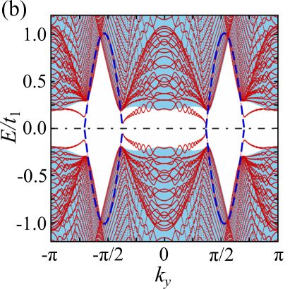
(b)

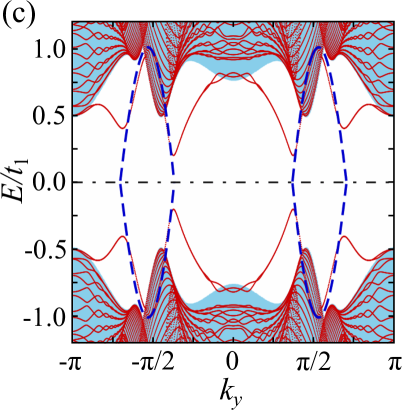
(c)

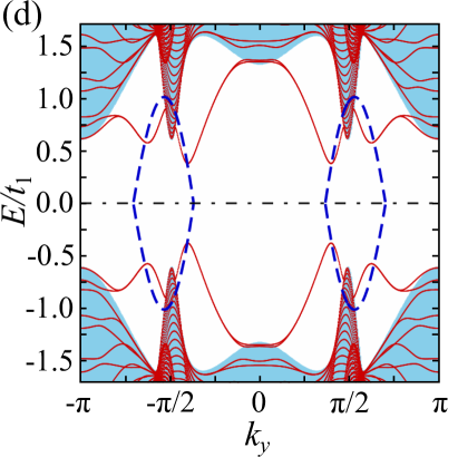
(d)

Figure 3: (Color online) Quasi-particle spectra in the superconducting phase for the two-orbital model. Bands of a (10) strip of width $W=40$ (red) are compared to the bulk bands projected onto the 1D BZ for the strip (blue). Only the low-energy part of the spectra is shown. (a) $\Delta=0.5$ for $s_{++}$-wave pairing. For comparison, the topological surface bands, modified according to $\xi\to\pm\sqrt{\xi^{2}+|\Delta|^{2}}$, are also plotted (dashed green lines). (b) $\Delta=0.5$ for $s_{\pm}$-wave pairing, (c) $\Delta=2.0$ for $s_{\pm}$-wave pairing, (d) $\Delta=6.0$ for $s_{\pm}$-wave pairing. In panels (b)–(d), the dashed dark blue lines denote topological surface bands of the normal state.

We now consider the superconducting phase, starting with the two-orbital model. Quasi-particle spectra of the superconducting (10) strip are shown for $s_{++}$-wave pairing in Fig. 3(a) and for $s_{\pm}$-wave pairing in Figs. 3(b)–(d). In all cases, the bands for the strip are compared to the bulk bands projected onto the 1D BZ for the strip. Large values of the gap $\Delta$ have been considered to more clearly exhibit the effects of interest. The spectra show the typical doubling and particle-hole symmetry induced by the BdG description.

In the case of $s_{++}$-wave pairing, a full gap opens without any edge states inside the gap. The bulk states are pushed out of the gap according to $\xi\to\pm\sqrt{\xi^{2}+|\Delta|^{2}}$. Interestingly, the surface bands are modified in the same way, as emphasized by the dashed green lines in Fig. 3(a). We can understand this by noting that the $s_{++}$-wave pairing interaction is purely local and is therefore not affected by the introduction of edges. Hence, one would indeed expect $s_{++}$-wave pairing to induce similar gaps for bulk and surface states. In this process, the edge bands from the normal state (dashed green lines) become resonant with bulk states, which destroys their localization at the edges. Moreover, there are no Andreev bound states. This is expected since for Andreev bound states to appear Andreev reflection involving gaps of opposite sign has to be possible.KaT00

Let us now discuss the realistic case of $s_{\pm}$-wave superconductivity. First, Figs. 3(b)–(d) show that the bulk gap is no longer constant in the BZ. Moreover, there are states inside the bulk gap. In contrast to the $s_{++}$-wave case, the topological surface bands from the normal state are not pushed away. In fact, they coincide closely with the normal-state bands and their charge conjugates, as indicated by the dashed dark blue lines. Although they are still mostly hidden in the bulk continuum in Fig. 3(b), parts of them become visible within the gap. Near zero energy, we observe a gap for the surface bands, which is much smaller than the bulk gap. Furthermore, we find additional edge bands in ranges of $k_{y}$ without edge states in the normal phase, but connected to them. They merge with the bulk continuum at $k_{y}=0$ and $k_{y}=\pi$. On the whole, there is a pair of surface bands for $E>0$, doubled at $E<0$. Within the pairs, we find bonding and anti-bonding states whose energy difference is exponentially small for large width.

It is reasonable that $s_{\pm}$-wave and $s_{++}$-wave pairing differently affect the surface states resulting from the normal phase. The $s_{\pm}$-wave pairing interaction is not local but connects next-nearest-neighbor sites. Thus, the interaction is cut off at the edges so that it affects edge states less strongly than bulk states.

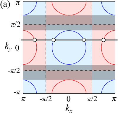
(a)

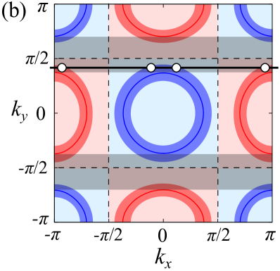
(b)

Figure 4: (Color online) Scattering processes in the two-orbital model for the (10) strip. The shaded regions indicate $k_{y}$ values for which surface states of topological origin exist in the normal, paramagnetic phase. The bold lines are exemplary lines with constant $k_{y}$ for which sign-changing scattering processes are possible. Relevant states are indicated by white circles. (a) Small $\Delta$: sign-changing processes can only occur outside of the shaded regions. Topological states and Andreev bound states are separated. (b) Larger $\Delta$: states in a broader region around the Fermi surfaces become relevant. Topological states merge with Andreev bound states.

The additional surface bands can be explained as Andreev bound states:KaT00 ; OnT09 ; NaH09 The Fermi surface of the normal state along with the sign structure of the gap function are illustrated in Fig. 4. The edge is parallel to the $y$ axis and, hence, $k_{y}$ is a constant of motion during the scattering processes. Therefore, we have to consider lines through the BZ with constant $k_{y}$ in order to find the available states. Furthermore, for small gap amplitudes $\Delta$, only states at the Fermi surfaces are relevant. From Fig. 4(a), we see that sign-changing scattering processes are possible for all $k_{y}$ except where the line $k_{y}=\mathrm{const}$ does not cross a Fermi surface. But the latter is exactly the region where we have found topological surface states. In other words, topological states are only possible if the $k_{y}=\mathrm{const}$ line corresponds to a gapped system with no states available at the Fermi energy, whereas Andreev states require a gapless system where states at the Fermi level do exist. Hence, topological surface states inherited from the normal phase and Andreev bound states coexist, but their $k_{y}$ ranges do not overlap in the limit of small $\Delta$.

Note that the bands of topological states and of Andreev bound states are connected. This is easy to understand: As discussed above, the bands of topological surface states are less strongly affected by the nonlocal $s_{\pm}$-wave pairing. On the other hand, the bands must be continuous in $k_{y}$ and thus cannot suddenly terminate. Consequently, in the superconducting state additional states must appear in the gap that complete the bands of topological states.

For larger $\Delta$, states from a broader range of $\mathbf{k}$ values in the vicinity of the normal-state Fermi surface are relevant for Andreev scattering, as illustrated by Fig. 4(b). Consequently, the $k_{y}$ range for Andreev bound states grows, as does the transition region between them and the topological surfaces states. In Figs. 3(b)–(d), the effect of a growing gap amplitude is depicted. We observe that the gap in the surface bands gets larger. Moreover, in the $k_{y}$ range for topological surface states, the edge bands lose their resemblance to the normal state (dashed dark blue lines). This is due to both the large gap amplitude, which now strongly affects also the topological surface states, and the growing contribution of Andreev scattering.

The bands of Andreev bound states in Fig. 3 are similar to the ones found in Ref. HuL10, . They are also qualitatively similar to the bands in Ref. OnT09, for the (11) edge, which corresponds to our (10) edge due to the $45^{\circ}$ rotation of the BZ. Surface states resulting from the normal phase are not addressed in either work.

(a)

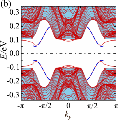
(b)

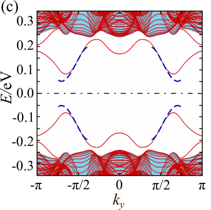
(c)

Figure 5: (Color online) Quasi-particle spectra in the superconducting phase for the five-orbital model. Bands of a (10) strip of width $W=40$ (red) are compared to the bulk bands projected onto the 1D BZ for the strip (blue). Only the low-energy part of the spectra is shown. (a) $\Delta=0.15$ ($s_{++}$ pairing). For comparison, some of the topological surface bands modified according to $\xi\to\pm\sqrt{\xi^{2}+|\Delta|^{2}}$ are also plotted (dashed green lines). (b) $\Delta=0.15$ ($s_{\pm}$ pairing), (c) $\Delta=0.4$ ($s_{\pm}$ pairing). In panels (b) and (c), the dashed dark blue lines denote topological surface bands of the normal state.

We now turn to the five-orbital model. Quasi-particle spectra of the superconducting (10) strip are shown for $s_{++}$-wave pairing in Fig. 5(a) and for $s_{\pm}$-wave pairing in Figs. 5(b), (c). For $s_{++}$-wave pairing, we observe that bulk and surface states are affected similarly by superconductivity, as for the two-orbital model. In the five-orbital model, there are two bundles of surface bands in the normal, paramagnetic phase.LaT13 In the $s_{++}$-wave superconducting state, one of these bundles vanishes in the bulk continuum. However, in contrast to the two-orbital model, the lower bundle remains visible in the bulk gap. Its dispersion is well represented by modifying the normal-state band according to $\xi\to\pm\sqrt{\xi^{2}+|\Delta|^{2}}$ (dashed green lines). Andreev bound states are not present due to the absence of sign-changing scattering processes.

The case of $s_{\pm}$-wave superconductivity is illustrated in Figs. 5(b), (c). Like for the two-orbital model, we see that the topological surface bands are hardly affected by superconductivity, except close to the Fermi energy, where the bands are pushed to higher energies. The effect is weaker than for the two-orbital model because the normal-state surface bands do not lie close to the Fermi energy. The higher-energy topological surface band is not visible since it is resonant with the bulk continuum. Like for the two-orbital model, we observe Andreev bound states outside of the $k_{y}$ range for which we have found topological edge states in the normal phase. The explanation is analogous to the two-orbital model. For increasing gap amplitude, the Andreev bound states merge with the lower-energy topological surface band, which loses its resemblance to the normal state, as for the two-orbital model. Eventually, the entire band separates from the bulk continuum, as seen in Fig. 5(c). Along with this, a second band of Andreev bound states appears.

III.2 Strips with (11) edges

Paramagnetic and antiferromagnetic phase

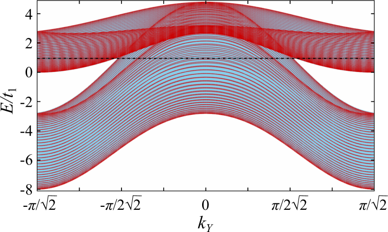
Figure 6: (Color online) Energy bands in the paramagnetic phase for the two-orbital model. Bands of a (11) strip of width $W=40$ (red) are compared to the bulk bands projected onto the 1D BZ for the strip (blue). The black dash-dotted line denotes the Fermi energy at half filling.

For the (11) strip, we begin with the discussion of the two-orbital model. In Fig. 6, the energy dispersion of the paramagnetic strip is plotted along with the energies of the extended system projected onto this BZ. We find energy gaps close to the borders of the BZ. However, there are no edge bands for the paramagnetic (11) strip. The same holds for the SDW phase (not shown).

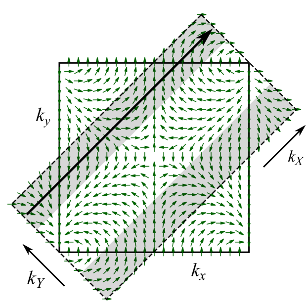
Figure 7: (Color online) Vector field $(\cos\phi(\mathbf{k}),\sin\phi(\mathbf{k}))$ (green arrows) and exemplary path at constant $k_{Y}$ (black arrow) in the extended BZ. The shaded regions are the areas for which an effective 1D system with fixed $k_{Y}$ has a bulk gap. The gap is not necessarily at the Fermi energy.

We can understand the absence of surface states from a topological perspective. The argument is similar to the one for the (10) strip.LaT13 Following Ran et al.,RWZ09 we rewrite Eq. (1) as $\mathcal{H}^{0}(\mathbf{k})=a(\mathbf{k})\,\tau^{0}+b(\mathbf{k})\,[\sin\phi(\mathbf{k})\,\tau^{1}+\cos\phi(\mathbf{k})\,\tau^{3}]$. In Ref. LaT13, , we have considered the winding of $\phi(\mathbf{k})$ at constant $k_{y}$. For the (11) strip, we have to analyze paths through the BZ at constant $k_{Y}$, i.e., diagonal lines through the BZ associated with the unrotated unit cell, as illustrated in Fig. 7. We see immediately that the winding number for $\phi(\mathbf{k})$ vanishes for all relevant paths. Hence, a continuous deformation of the Hamiltonian similar to the (10) case, establishing particle-hole and time-reversal symmetry without closing the gap, leads to a Hamiltonian in Altland-Zirnbauer class BDI,Zir96 ; SRF08 but with a trivial topological invariant of $n=0$. Thus, there are no zero-energy end states in the corresponding finite chain and we do not obtain edge states after reversing the deformation.

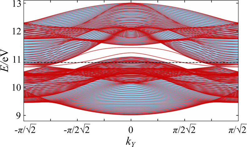
Figure 8: (Color online) Energy bands in the paramagnetic phase for the five-orbital model. Bands of a (11) strip of width $W=20$ (red) are compared to the bulk bands projected onto the 1D BZ for the strip (blue). The black dash-dotted line denotes the Fermi energy at filling factor $0.6$.

For the five-orbital model, Fig. 8 shows the band structure of the system along with the projected bulk spectrum. Contrary to the results in the two-orbital model, there are two bundles of surface bands. They are connected to the bulk bands at the projected Dirac points of the paramagnetic system, which do not exist in the two-orbital model. Like for the (10) edge, each bundle consists of two pairs of degenerate states with exponentially small splitting between them for large $W$.

The existence of edge states for the (11) strip can again be understood based on a topological argument:LaT13 We obtain effective 1D Hamiltonians by considering paths through the BZ at constant $k_{Y}$. Edge states could in principle exist whenever there is a gap in the bulk spectrum for this value of $k_{Y}$. This is the case for all $k_{Y}$ except where the path contains Dirac points, at $k_{Y}\approx\pm 1.8$, see Fig. 8. There are two classes of gapped 1D Hamiltonians: the ones for $k_{Y}$ in the interval spanned by the projected Dirac points and the ones outside of this interval. We consider one representative for each class, corresponding to the paths $\mathcal{C}_{1}$ at $k_{Y}=0$ and $\mathcal{C}_{2}$ at $k_{Y}=\pi/\sqrt{2}$, respectively. All of the following deformations are continuous and do not close the energy gap. We first decouple the $3d_{3Z^{2}-R^{2}}$ orbital from the others in order to get effective four-orbital Hamiltonians. We then tune all on-site energies and all hopping amplitudes beyond next-nearest neighbors to zero. The components of the $4\times 4$ matrices now consist of linear combinations of $\cos k$, $\cos 2k$, $\sin k$, $\sin 2k$, and constant terms.

For the Hamiltonian for the path $\mathcal{C}_{1}$, we continue by tuning the $\cos 2k$, $\sin 2k$ and the constant terms to zero. After tuning all remaining coefficients to $1/4$, the resulting matrix is unitarily equivalent to

$$\hat{\mathcal{H}}_{1}(k)=\begin{pmatrix}0&e^{-ik}&0&0\\ e^{ik}&0&0&0\\ 0&0&0&e^{-ik}\\ 0&0&e^{ik}&0\end{pmatrix},$$ (8)

which consists of two topologically nontrivial two-orbital systems in class BDIZir96 ; SRF08 with winding numbers $n=1$. This deformed model has four zero-energy edge bands, two at each edge. These numbers are doubled if we include the spin. Upon reversing the deformation, the symmetries defining the class BDI are lost so that the edge states are no longer required to have zero energy. The edge bands thus become dispersive. The degeneracy between the two sectors in Eq. (8) is also broken and we therefore end up with two bundles of edge states.

For the path $\mathcal{C}_{2}$, we tune all nonzero hopping parameters to the same value denoted by $t$. This is followed by smoothly tuning the vanishing matrix elements between $3d_{X^{2}-Y^{2}}$ and $3d_{XY}$ to $-2t\cos k$. Next, the $\cos 2k$, $\sin 2k$, and constant terms are tuned to zero. After fixing $t$ to $1/2$ and a unitary transformation we obtain the block Hamiltonian

$$\hat{\mathcal{H}}_{2}(k)=\begin{pmatrix}0&e^{-ik}&0&0\\ e^{ik}&0&0&0\\ 0&0&0&-e^{-ik}\\ 0&0&-e^{ik}&0\end{pmatrix},$$ (9)

which comprises two topologically nontrivial two-orbital systems with winding numbers $n=1$. This deformed system has the same number of zero-energy edge bands as $\hat{\mathcal{H}}_{1}(k)$ and the original system thus has two bundles of edge states also in this $k_{Y}$ range.

In the antiferromagnetic phase, the 1D surface BZ is halfed due to the ordering vector $\mathbf{Q}^{\prime}=(\pi/\sqrt{2},-\pi/\sqrt{2})$ in the rotated $(k_{X},k_{Y})$ coordinate system. Hence, the number of bands is doubled and one would in principle find four bundles of surface bands. However, two of them become resonant with the bulk states. The degeneracy of the remaining two bundles at the boundaries of the new BZ is lifted by the SDW. Moreover, we find that the original four-fold degeneracy for $W\to\infty$ is still intact, since the magnetization at the (11) edge is staggered. All of this is similar to the (01) case discussed above.

Superconducting phase

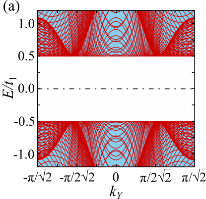
(a)

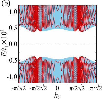
(b)

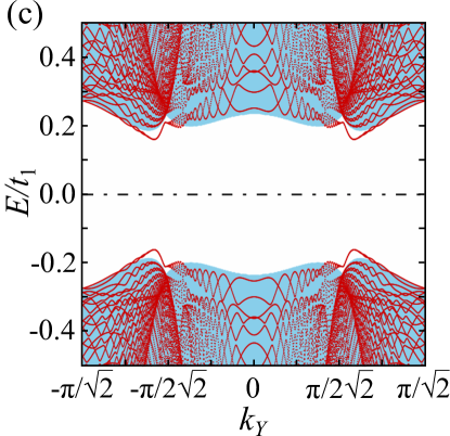
(c)

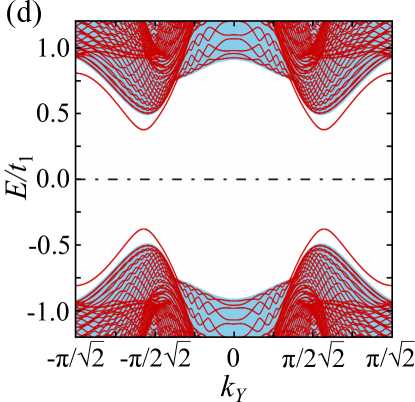
(d)

Figure 9: (Color online) Quasi-particle spectra in the superconducting phase for the two-orbital model. Bands of a (11) strip of width $W=40$ (red) are compared to the bulk bands projected onto the 1D BZ for the strip (blue). (a) $\Delta=0.5$ ($s_{++}$ pairing), (b) $\Delta=0.1$ ($s_{\pm}$ pairing), (c) $\Delta=0.5$ ($s_{\pm}$ pairing), (d) $\Delta=2.0$ ($s_{\pm}$ pairing). Only the low-energy part of the spectra is shown. Note that there were no surface states in the normal phase, see Fig. 6.

For the superconducting phase, we start with the two-orbital model. In the superconducting phase with $s_{++}$-wave gap, no surface states appear, see Fig. 9(a). This is expected since, on the one hand, this model does not have edge states at the (11) edge in the normal phase and, on the other, the condition for the existence of Andreev bound states is not satisfied.

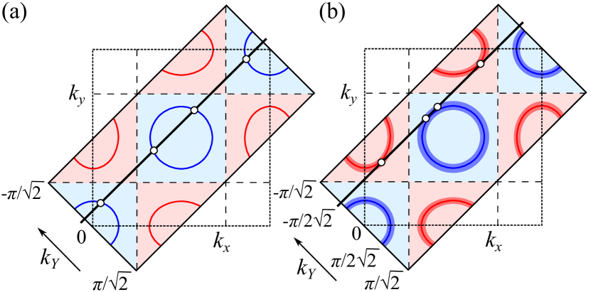
Figure 10: (Color online) Scattering processes in the two-orbital model for the (11) strip. The extended BZ is illustrated along with the Fermi surfaces. The bold lines are exemplary lines with constant $k_{Y}$. Relevant states are drawn as white circles. (a) Small $\Delta$: Sign-changing processes can never occur. (b) Larger $\Delta$: Relevant states are also found in the vicinity of the Fermi surfaces and sign-changing scattering processes become possible. Andreev bound states can emerge.

In the case of $s_{\pm}$-wave pairing, there are no surface states for a small gap $\Delta$ as shown in Fig. 9(b). This can again be understood from evaluating the sign-changing condition for Andreev bound states. We consider paths through the extended BZ at constant $k_{Y}$, see Fig. 10(a). All such lines either cross Fermi pockets with the same sign or do not cross a Fermi surface at all. Hence, sign-changing scattering processes are not possible if the gap is small and one does not find Andreev bound states. For larger $\Delta$, also states away from the Fermi surface become relevant, as indicated in Fig. 10(b). Thus, scattering processes with a sign change of the gap function can occur, leading to the emergence of Andreev bound states. In this case, the Andreev states are of course not connected to topological states.

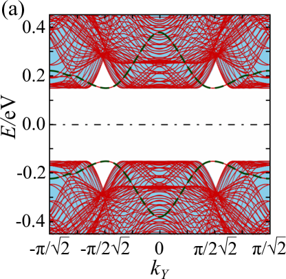
(a)

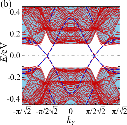
(b)

Figure 11: (Color online) Quasi-particle spectra in the superconducting phase for the five-orbital model. Bands of a (11) strip of width $W=20$ (red) are compared to the bulk bands projected onto the 1D BZ for the strip (blue). Only the low-energy part of the spectra is shown. (a) $\Delta=0.15$ ($s_{++}$ pairing). For comparison, some of the topological surface bands modified according to $\xi\to\pm\sqrt{\xi^{2}+|\Delta|^{2}}$ are also plotted (dashed green lines). (b) $\Delta=0.15$ ($s_{\pm}$ pairing). The dashed dark blue lines denote topological surface bands of the normal state.

Finally, we turn to the superconducting (11) strip in the five-orbital model. In Fig. 8, we found two bundles of surface states in the normal phase. In the superconducting state, the upper bundle vanishes completely into the bulk continuum, whereas the lower bundle remains partly in a bulk gap. This is similar to the (10) system in the five-orbital model. However, the present case is particularly interesting since the normal-state edge bands cross the Fermi energy.

For $s_{++}$-wave superconductivity, bulk and edge states are again gapped in the same way, see Fig. 11(a). For $s_{\pm}$-wave pairing, we observe that a larger part of the lower bundle of topological surface bands remains inside the gap, hardly affected by the superconducting pairing, see Fig. 11(b). However, a very small gap opens, which is much smaller than the bulk gap. This can again be attributed to the weakening of the nonlocal $s_{\pm}$-wave pairing interaction at the edge, discussed in Sec. III.1.

Furthermore, we find additional surface bands near $k_{Y}=\pm\pi/2\sqrt{2}$ very close to the bulk continuum. These can be understood as Andreev bound states as discussed for the two-orbital model. We note that the behavior of the surface bands for larger $\Delta$, is similar to the (10) strip. The surface band gap grows and the resemblance of the topological bands to the normal phase gets weaker (not shown). In addition, the Andreev bands separate more strongly from the bulk continuum.

IV Conclusions

We have studied various strip geometries of iron pnictides with small-index edges in the paramagnetic, antiferromagnetic, and superconducting phases with regard to the possible existence of surface states. For this, we have used both a simple two-orbital modelRWZ09 and a more realistic five-orbital model.KOA08

For the paramagnetic phase, we have found that the number of surface bands depends both on the strip geometry and the specific model considered. The (10) strip shows edge states in both models.LaT13 The two-orbital model predicts one spin-degenerate band of edge states at each edge (in the limit of large width), resulting from nontrivial winding in the $3d_{XZ}$, $3d_{YZ}$ orbital space. The five-orbital model has additional nontrivial winding with regard to the $3d_{X^{2}-Y^{2}}$ and $3d_{XY}$ orbitals, which doubles the number of edge bands.LaT13 The results for the (11) strip show that also the winding in the sector of $3d_{XZ}$ and $3d_{YZ}$ is different between the two models: the two-orbital model is topologically trivial and thus has no edge states, whereas the five-orbital model has two spin-degenerate edge bands at each (11) edge. This indicates that the two-orbital model is too simple to account for the full topological structure of the pnictide bands.

The presence or absence of surface states can be explained by considering a continuous deformation of effective 1D Hamiltonians into Hamiltonians in symmetry class BDI.Zir96 ; SRF08 ; LaT13 However, these states are no longer topologically protected and thus move away from the Fermi energy when the deformation is reversed. It is worth pointing out that this type of argument is rather robust since it only relies on the existence of a continuous deformation that does not close a gap. Therefore, the qualitative results, in particular the existence of surface states, would not change if we included (i) changes in the model parameters close to the surface, describing possible reconstruction and relaxation, (ii) order parameters $m_{ab}$ and $\Delta$ calculated self-consistently for the strip geometry, or (iii) weak coupling in the third dimension.

In the antiferromagnetic phase, the degeneracy of the surface bands in the limit of large width is strongly lifted if the presence of the SDW leads to a net spin polarization of the edges, which for $(\pi,0)$ order is the case for $(10)$ edges but not for $(01)$ or $(11)$ edges. Nevertheless, the remaining two-fold degeneracy is protected by a combination of spin rotation and spatial reflection.

In the superconducting phase with $s_{\pm}$-wave gap structure, the topological surface states are less strongly affected by the superconducting pairing than the bulk states. Only a small gap opens in the surface bands so that they are almost identical to the normal state and partially remain inside the gap. In addition, Andreev bound states appear for certain edges, which can be understood from the changing gap sign for Andreev reflection.KaT00 ; OnT09 ; NaH09 ; NHM10 ; HuL10 For small gaps, the Andreev bound states coexist with the topological states in different ranges of the momentum component parallel to the edge. For larger—and for pnictides unphysical—gap values, the Andreev bound states and topological surface bands merge and lose their individual character.

The edges studied here correspond to (100), (110), and (010) surfaces in the real three-dimensional system. However, these surfaces are challenging to prepare since the natural cleavage plane is (001). More promising is the examination of single-unit-cell steps on pnictide (001) surfaces, which are indeed occasionally seen in scanning-tunneling-microscopy experiments.Hess Since the coupling between layers in 1111 pnictides is weak, it would only weakly perturb the bound states at the edge of the incomplete layer. Hence, it should be possible to detect bound states at step edges with scanning tunneling spectroscopy. For the detection of bound states in the superconducting phase, it might be possible to perform tunneling experiments on normal-superconducting interfaces at the edges of a (001) pnictide sample.

On a more general level, our results emphasize that topological signatures, such as surface states, can occur in materials that are not topological in the sense of the topological classification of gapped systems.SRF08 Iron pnictides and graphene are examples of gapless materials that have topological properties. In the pnictides, the topologically nontrivial properties come from the multi-orbital character of the band structure close to the Fermi energy. It is promising to search for other materials with topological features related to their multi-orbital structure.

References

- (1) D. Johnston, Adv. Phys. 59, 803 (2010).
- (2) P. Dai, J. Hu, and E. Dagotto, Nature Phys. 8, 709 (2012).
- (3) M. Z. Hasan and C. L. Kane, Rev. Mod. Phys. 82, 3045 (2010).
- (4) X.-L. Qi and S.-C. Zhang, Rev. Mod. Phys. 83, 1057 (2011).
- (5) A. Lau and C. Timm, Phys. Rev. B 88, 165402 (2013).
- (6) Y. Ran, F. Wang, H. Zhai, A. Vishwanath, and D.-H. Lee, Phys. Rev. B 79, 014505 (2009).
- (7) A. H. Castro Neto, F. Guinea, N. M. R. Peres, K. S. Novoselov, and A. K. Geim, Rev. Mod. Phys. 81, 109 (2009).
- (8) J. Kunstmann, C. Özdoğan, A. Quandt, and H. Fehske, Phys. Rev. B 83, 045414 (2011).
- (9) M. S. Tokikachvili, S. L. Bud’ko, N. Ni, and P. C. Canfield, Phys. Rev. Lett. 101, 057006 (2008).
- (10) H. Luetkens, H.-H. Klauss, M. Kraken, F. J. Litterst, T. Dellmann, R. Klingeler, C. Hess, R. Khasanov, A. Amato, C. Baines, M. Kosmala, O. J. Schumann, M. Braden, J. Hamann-Borrero, N. Leps, A. Kondrat, G. Behr, J. Werner, and B. Büchner, Nature Mat. 8, 305 (2009).
- (11) D. K. Pratt, W. Tian, A. Kreyssig, J. L. Zarestky, S. Nandi, N. Ni, S. L. Bud’ko, P. C. Canfield, A. I. Godman, and R. J. McQueeney, Phys. Rev. Lett. 103, 087001 (2009).
- (12) T. Goko, A. A. Aczel, E. Baggio-Saitovitch, S. L. Bud’ko, P. C. Canfield, J. P. Carlo, G. F. Chen, P. Dai, A. C. Hamann, W. Z. Hu, H. Kageyama, G. M. Luke, J. L. Luo, B. Nachumi, N. Ni, D. Reznik, D. R. Sanchez-Candela, A. T. Savici, K. J. Sikes, N. L. Wang, C. R. Wibe, T. J. Williams, T. Yamamoto, W. Yu, and Y. J. Uemura, Phys. Rev. B 80, 024508 (2009).
- (13) M. D. Lumsden and A. D. Christianson, J. Phys.: Condens. Matter 22, 203203 (2010).
- (14) E. Wiesenmayer, H. Luetkens, G. Pascua, R. Khasanov, A. Amato, H. Potts, B. Banusch, H.-H. Klauss, and D. Johrendt, Phys. Rev. Lett. 107, 237001 (2011).
- (15) S. Avci, O. Chmaissem, E. A. Gremychkin, S. Rosenkranz, J.-P. Castellan, D. Y. Chng, I. S. Todorov, J. A. Schluedter, H. Claus, M. G. Kanatzidis, A. Daoud-Aladine, D. Khalyavin, and R. Osborn, Phys. Rev. B 83, 172503 (2011).
- (16) P. J. Hirschfeld, M. M. Korshunov, and I. I. Mazin, Rep. Prog. Phys. 74, 124508 (2011).
- (17) A. V. Chubukov, Ann. Rev. Condens. Matter Phys. 3, 57 (2012).
- (18) S. Onari and Y. Tanaka, Phys. Rev. B 79, 174526 (2009).
- (19) Y. Nagai and N. Hayashi, Phys. Rev. B 79, 224508 (2009).
- (20) Y. Nagai, N. Hayashi, and M. Machida, Physica C 470, S504 (2010).
- (21) W.-M. Huang and H.-H. Lin, Phys. Rev. B 81, 052504 (2010).
- (22) K. Kuroki, S. Onari, R. Arita, H. Usui, Y. Tanaka, H. Kontani, and H. Aoki, Phys. Rev. Lett. 101, 087004 (2008).
- (23) S. Kashiwaya and Y. Tanaka, Rep. Prog. Phys. 63, 1641 (2000).
- (24) M. R. Zirnbauer, J. Math. Phys. 37, 4986 (1996); A. Altland and M. R. Zirnbauer, Phys. Rev. B 55, 1142 (1997).
- (25) A. P. Schnyder, S. Ryu, A. Furusaki, and A. W. W. Ludwig, Phys. Rev. B 78, 195125 (2008); A. Y. Kitaev, AIP Conf. Proc. 1134, 22 (2009).
- (26) C. Hess (private communication).