A first-principles-based correlation functional for harmonious connection of short-range correlation and long-range dispersion

Abstract

We present a physically motivated correlation functional belonging to the meta-generalized gradient approximation (meta-GGA) rung, which can be supplemented with long-range dispersion corrections without introducing double-counting of correlation contributions. The functional is derived by the method of constraint satisfaction, starting from an analytical expression for a real-space spin-resolved correlation hole. The model contains a position-dependent function that controls the range of the interelectronic correlations described by the semilocal functional. With minimal empiricism, this function may be adjusted so that the correlation model blends with a specific dispersion correction describing long-range contributions. For a preliminary assessment, our functional has been combined with the DFT-D3 dispersion correction and full Hartree-Fock (HF)-like exchange. Despite the HF-exchange approximation, its predictions compare favorably with reference interaction energies in an extensive set of non-covalently bound dimers.

I Introduction

Inclusion of the dispersion interactions into the set of phenomena accounted for by DFT models is recognized as one of the challenges in the development of new density functional approximations (DFAs).Dobson (2012); Dobson et al. (2005); Cohen, Mori-Sánchez, and Yang (2012); Dobson and Gould (2012) Several ways have been proposed to correct the currently available semilocal (SL) DFAs for the lacking nonlocal (NL) correlation contribution responsible for the dispersion interactions.Cohen, Mori-Sánchez, and Yang (2012); Dobson (2012) Hereafter, global hybrid and range-separated hybrid functionals will be called SL DFAs. Although the exchange parts of such functionals are nonlocal, our focus will be on the correlation contributions, which in this case depend on variables calculated at a single point of space. The examples of such dispersion-corrected methods are: (i) the exchange-hole dipole method (XDM),Becke and Johnson (2005a, b, 2007); Heßelmann (2009); Ángyán (2007) (ii) the atom pairwise additive schemes of Goerigk and Grimme, DFT-D3,Grimme et al. (2010) and Tkatchenko-Scheffler approach,Tkatchenko and Scheffler (2009) (iii) seamless van der Waals density functionals.Dion et al. (2004); Lee et al. (2010); Vydrov and Van Voorhis (2009a, b, 2010a); Vydrov and Voorhis (2012); Dobson and Gould (2012) It is clear that the accuracy of these methods depends not only on a faithful representation of long-range electronic correlations, but also on a consistent matching of a dispersion correction and the chosen SL complement.

Several groups have studied the conditions under which an SL functional can be incorporated into a dispersion-corrected method.Pernal et al. (2009); Rajchel et al. (2010); Kamiya, Tsuneda, and Hirao (2002); Murray, Lee, and Langreth (2009) It has been concluded that the improper behavior of a GGA exchange functional in the density tail (large reduced gradient regime) is responsible for artificial exchange binding (as for the PBEPerdew, Burke, and Ernzerhof (1996) exchange) or overly repulsive interaction (as for the B88Becke (1988a) exchange).Kamiya, Tsuneda, and Hirao (2002); Murray, Lee, and Langreth (2009) Such systematic errors may cause the NL correction to worsen the results compared to the bare SL functional. The following exchange functionals: PW86,Perdew and Yue (1986) refitted PW86,Murray, Lee, and Langreth (2009) and range-separated hybridsKamiya, Tsuneda, and Hirao (2002); Vydrov and Van Voorhis (2010a) were found to be free from artificial binding, thus being consistent with NL dispersion correction. Similarly, combining exact exchange with NL correlation performs satisfactorily.Vydrov and Van Voorhis (2010b)

It has been observed that a failure to satisfy the condition of vanishing correlation for a rapidly varying density by SL correlation functionalsPerdew, Burke, and Ernzerhof (1996) leads to a systematic overbinding of non-covalent complexes.Kamiya, Tsuneda, and Hirao (2002) The ad hoc cure is to cancel the error of the correlation by the opposite-sign error of an exchange component.Kamiya, Tsuneda, and Hirao (2002) However, this does not resolve the problem of the double counting of SL and NL correlation. Several remedies have been proposed. For atom pairwise schemes, multiple damping functions have been devised.Grimme and Ehrlich (2011) For VV09Vydrov and Van Voorhis (2009b) and VV10Vydrov and Van Voorhis (2010a) density functionals the problem is avoided by demanding the NL constituent to vanish in the homogeneous electron gas (HEG) limit, because the SL constituent is able to describe the whole range of the electronic interactions in this limit. Finally, Pernal et al. (2009) devised a procedure to reoptimize an existing SL exchange-correlation functional so as to recover the dispersionless interaction energy.Pernal et al. (2009) The rationale of such an approach is to let the SL functional contribute only the terms that it can describe reliably.

At this point we would like to shed light on the dispersion problemDobson et al. (2002) in DFT. It has been well established that SL functionals fail to recover the long-range multipole-expanded dispersion energy. In fact, nearly all dispersion-corrected DFT approaches aim at recovering only long-range dispersion, roughly determined by the leading terms of the multipole expansion: $C_{6}$, and possibly $C_{8}$. The exceptions are the approaches of Pernal et al. (2009) and and Rajchel et al. (2010) which supplement an SL functional with total non-expanded dispersion from SAPT. It is often overlooked that the long-range contribution, however, does not constitute the whole dispersion energy at near-equilibrium distances. Setting aside the exchange-dispersion part, the dispersion energy, as defined in the symmetry-adapted perturbation theory (SAPT),Hesselmann and Jansen (2003); Misquitta et al. (2005) has a complex nature, and includes both long- and short-range contributions. This has first been observed by Koide (1976) who quantified the short-distance behavior of the dispersion energy as $A+BR^{2}$, with $R$ being the intermonomer separation. The importance of the short-range correlation is also unambiguously, though indirectly, supported by the significance of bond functions and explicitly correlated Gaussian geminals in the dispersion energy calculations.Burcl et al. (1995) A more direct argument points to the existence of short-range terms in the exact angular expansion of the dispersion energy. In the case of atomic interactions, the latter involves the interaction between $S$ states of monomers,Koide (1976) which give no contribution to the multipole expansion. Numerical results show that near the equilibrium bond length these terms, decaying exponentially with the overlap density, can be comparable in magnitude to the multipole expansion terms.Koide, Meath, and Allnatt (1981) As demonstrated by Dobson et al. (2002) with the aid of simple models, SL functionals cannot recover the multipole expansion of the dispersion energy. However, there is a good reason to believe that SL functionals are capable of describing the terms that depend on overlap density.Dobson et al. (2002) Our model is intended to capture this contribution.

Recent thorough assessments of DFT-D, XDM, and VV10 approaches have clearly shown that a combination of an SL functional specifically designed for a dispersion-corrected treatment with a dispersion correction improves both the description of noncovalent interactionsBurns et al. (2011); Goerigk and Grimme (2011); Hujo and Grimme (2011); Vazquez-Mayagoitia et al. (2010); Thanthiriwatte et al. (2011) and general molecular properties.Goerigk and Grimme (2011); Hujo and Grimme (2011) Among the functionals that use atom-pairwise DFT-D correction, B97-D,Grimme (2006) B97-D3,Goerigk and Grimme (2011) and $\omega$-B97X-DChai and Head-Gordon (2008a, b) are characterized by one of the smallest magnitude and spread of errors in interaction energiesBurns et al. (2011) while performing well in thermochemistry and reaction kinetics. The methods utilizing unaltered conventional SL functional suffer from systematic errors. For example, PBE0-D2, PBE-D3, and B3LYP-D3 tend to underbind dispersion-bound complexes and overbind hydrogen-bonded systems.Burns et al. (2011) The systematic overbinding of charge-transfer complexes within DFT is more pronounced for the dispersion-corrected approaches than for the pure DFAs.Ruiz, Salahub, and Vela (1996); Sini, Sears, and Bredas (2011) See Ref.42 and Table 2 in Ref. 43, where numerical examples of huge overbinding by $\omega$-B97X-D and B97-D functionals applied to charge-transfer complexes are given.

Although much attention has been devoted to the development of the proper exchange contribution,Kamiya, Tsuneda, and Hirao (2002); Murray, Lee, and Langreth (2009); Swart, Solà, and Bickelhaupt (2009) the theoretical effort to derive a dispersion-consistent SL correlation functional thus far has been reduced to reoptimizing known expressions. It has also been observedGrimme (2006); Chai and Head-Gordon (2008b) that fitting to empirical data coupled with addition of higher-order terms in the B97 expansionBecke (1997) does not systematically improve the performance as the saturation is approached. Clearly, there is a demand for the theoretical effort to overcome the problem.

The aim of this work is to develop an SL correlation functional that can be matched with an arbitrary long-range dispersion correction by optimizing a single parameter that has a simple physical meaning. As a demonstration of this approach, we will combine our approximation with DFT-D3 dispersion correction,Grimme et al. (2010) which contributes damped $C_{6}/R^{6}+C_{8}/R^{8}$ terms, with no short-range contributions. To avoid the systematic error of spurious exchange attraction, full HF exchange will be used. To match SL and NL constituents, a function which controls the spatial extent of our SL correlation hole will be adjusted by minimization of errors in a relevant set of molecules.

II Theory

We consider an electronic ground state of a finite molecular system described by an electronic Hamiltonian of the form

$$\hat{H}=\hat{T}+\sum_{i}\hat{v}_{\mathrm{ext}}(\mathbf{r}_{i})+\hat{V}_{\mathrm{ee}},$$ (1)

where $\hat{T}$ is the kinetic energy operator, the multiplicative external potential $\hat{v}_{\mathrm{ext}}$ is taken to be the Coulomb potential of nuclear attraction, and $\hat{V}_{\mathrm{ee}}$ is the interelectronic repulsion. Atomic units are assumed throughout this work. In constrained-search formulationLevy (1979) of DFTHohenberg and Kohn (1964) the ground state energy of electronic system can be expressed as

$$E_{0}=\min_{\rho}\left[\int\hat{v}_{\mathrm{ext}}(\mathbf{r}_{1})\rho(\mathbf{r}_{1})\mathrm{d}^{3}\mathbf{r}_{1}+\left\langle\Psi^{\mathrm{min}}_{\rho}\middle|\hat{T}+\hat{V}_{\mathrm{ee}}\middle|\Psi^{\mathrm{min}}_{\rho}\right\rangle\right],$$ (2)

where $\Psi^{\mathrm{min}}_{\rho}$ denotes an $N$-body wavefunction that yields electronic density $\rho$ and simultaneously minimizes expectation value of $\hat{T}+\hat{V}_{\mathrm{ee}}$. In Kohn-Sham schemeKohn and Sham (1965) the second term on the right-hand side of Eq. (2) is decomposed into noninteracting kinetic, Hartree, and exchange-correlation energies, respectively:

$$\left\langle\Psi^{\mathrm{min}}_{\rho}\middle|\hat{T}+\hat{V}_{\mathrm{ee}}\middle|\Psi^{\mathrm{min}}_{\rho}\right\rangle=T_{\mathrm{s}}\left[\rho\right]+U\left[\rho\right]+E_{\mathrm{XC}}\left[\rho\right].$$ (3)

Noninteracting kinetic energy $T_{\mathrm{s}}$ is known explicitly in terms of the wavefunction of the KS system, denoted here as $\Phi^{\mathrm{min}}_{\rho}$, which merely minimizes the expectation value of $\hat{T}$:

$$T_{\mathrm{s}}\left[\rho\right]=\left\langle\Phi^{\mathrm{min}}_{\rho}\middle|\hat{T}\middle|\Phi^{\mathrm{min}}_{\rho}\right\rangle.$$ (4)

Hartree energy is given by a classical formula

$$U\left[\rho\right]=\frac{1}{2}\iint\frac{\rho(\mathbf{r}_{1})\rho(\mathbf{r}_{2})}{r_{12}}\mathrm{d}^{3}\mathbf{r}_{1}\mathrm{d}^{3}\mathbf{r}_{2}.$$ (5)

Exchange-correlation energy can be formally expressed through adiabatic connection formulaLevy (1996)

$$E_{\mathrm{XC}}\left[\rho\right]=\int_{0}^{1}\left\langle\Psi^{\mathrm{min,\lambda}}_{\rho}\middle|\hat{V}_{\mathrm{ee}}\middle|\Psi^{\mathrm{min,\lambda}}_{\rho}\right\rangle\mathrm{d}\lambda-U\left[\rho\right],$$ (6)

where $\Psi^{\mathrm{min,\lambda}}_{\rho}$ minimizes the expectation value of $\hat{T}+\lambda\hat{V}_{\mathrm{ee}}$ and yields the same electronic density as wavefunction at $\lambda=1$. Eq. (6) can be further decomposed so that the correlation energy is separately expressed through coupling-constant integral

$$E_{\mathrm{C}}\left[\rho\right]=\int_{0}^{1}V_{\mathrm{C}}^{\lambda}\left[\rho\right]\mathrm{d}\lambda$$ (7)

where

$$V_{\mathrm{C}}^{\lambda}\left[\rho\right]=\left\langle\Psi^{\mathrm{min,\lambda}}_{\rho}\middle|\hat{V}_{\mathrm{ee}}\middle|\Psi^{\mathrm{min,\lambda}}_{\rho}\right\rangle-\left\langle\Phi^{\mathrm{min}}_{\rho}\middle|\hat{V}_{\mathrm{ee}}\middle|\Phi^{\mathrm{min}}_{\rho}\right\rangle.$$ (8)

Approximating $V_{\mathrm{C}}^{\lambda}$ is the primary objective of this work. Let us begin by expressing $V_{\mathrm{C}}^{\lambda}$ in terms of a $\lambda$-dependent correlation hole

$$V_{\mathrm{C}}^{\lambda}=\frac{1}{2}\sum_{\sigma\sigma^{\prime}}\iint\frac{\rho_{\sigma}(\mathbf{r}_{1})h_{\mathrm{C}\lambda}^{\sigma\sigma^{\prime}}(\mathbf{r}_{1},\mathbf{r}_{2})}{r_{12}}\mathrm{d}^{3}\mathbf{r}_{1}\mathrm{d}^{3}\mathbf{r}_{2},$$ (9)

where $\sigma$ denotes a spin variable,

$$h_{\mathrm{C}\lambda}^{\sigma\sigma^{\prime}}(\mathbf{r}_{1},\mathbf{r}_{2})=h_{\mathrm{XC}\lambda}^{\sigma\sigma^{\prime}}(\mathbf{r}_{1},\mathbf{r}_{2})-h_{\mathrm{X}}^{\sigma\sigma^{\prime}}(\mathbf{r}_{1},\mathbf{r}_{2})$$ (10)

and

$$h_{\mathrm{XC}\lambda}^{\sigma\sigma^{\prime}}(\mathbf{r}_{1},\mathbf{r}_{2}) =\frac{P_{2\lambda}^{\sigma\sigma^{\prime}}(\mathbf{r}_{1},\mathbf{r}_{2})}{\rho_{\sigma}(\mathbf{r}_{1})}-\rho_{\sigma^{\prime}}(\mathbf{r}_{2}),$$ (11)

$$h_{\mathrm{X}}^{\sigma\sigma^{\prime}}(\mathbf{r}_{1},\mathbf{r}_{2}) =-\delta_{\sigma\sigma^{\prime}}\frac{\left|\sum_{i}^{N_{\sigma}}\psi_{i\sigma}^{*}(\mathbf{r}_{1})\psi_{i\sigma}(\mathbf{r}_{2})\right|^{2}}{\rho_{\sigma}(\mathbf{r}_{1})}.$$ (12)

$N_{\sigma}$ is a number of $\sigma$-spin electrons and pair probability density, $P_{2\lambda}^{\sigma\sigma^{\prime}}(\mathbf{r}_{1},\mathbf{r}_{2})$, is defined as

$$P_{2\lambda}^{\sigma\sigma^{\prime}}(\mathbf{r}_{1},\mathbf{r}_{2}) =N(N-1)$$

$$\times\sum_{\sigma_{3}\cdots\sigma_{N}}\int\Psi_{\rho}^{\min,\lambda*}(\mathbf{r}_{1}\sigma,\mathbf{r}_{2}\sigma^{\prime},\ldots,\mathbf{r}_{N}\sigma_{N})$$

$$\times\Psi_{\rho}^{\min,\lambda}(\mathbf{r}_{1}\sigma,\mathbf{r}_{2}\sigma^{\prime},\ldots,\mathbf{r}_{N}\sigma_{N})$$

$$\times\mathrm{d}^{3}\mathbf{r}_{3}\cdots\mathrm{d}^{3}\mathbf{r}_{N}.$$ (13)

Note that, due to the symmetry of $r_{\mathrm{ij}}^{-1}$ operator, it is the spherical average of exchange-correlation hole around the reference electron that enters the energy expression:

$$\begin{split}V_{\mathrm{C}}^{\sigma\sigma^{\prime},\lambda}&=\frac{1}{2}\iint\frac{\rho_{\sigma}(\mathbf{r}_{1})h_{\mathrm{C}\lambda}^{\sigma\sigma^{\prime}}(\mathbf{r}_{1},\mathbf{r}_{2})}{r_{12}}\mathrm{d}^{3}\mathbf{r}_{1}\mathrm{d}^{3}\mathbf{r}_{2}\\ &=\frac{1}{2}\int\mathrm{d}^{3}\mathbf{r}_{1}\int_{0}^{\infty}\frac{\rho_{\sigma}(\mathbf{r}_{1})h_{\mathrm{C}\lambda}^{\sigma\sigma^{\prime}}(\mathbf{r}_{1},s)}{s}4\pi s^{2}\mathrm{d}s\end{split}$$ (14)

where the spherical average is implied by scalar argument $s$,

$$h_{\mathrm{C}\lambda}^{\sigma\sigma^{\prime}}(\mathbf{r}_{1},s)=\frac{1}{4\pi}\int_{0}^{2\pi}\mathrm{d}\phi_{\mathbf{s}}\int_{0}^{\pi}h_{\mathrm{C}\lambda}^{\sigma\sigma^{\prime}}(\mathbf{r}_{1},\mathbf{r}_{1}+\mathbf{s})\sin\theta_{\mathbf{s}}\mathrm{d}\theta_{\mathbf{s}}.$$ (15)

Eq. (14) means that without loss of generality we can focus our attention on approximating isotropic quantity defined in Eq. (15).

We postulate the following form of opposite-spin and same-spin correlation holes:

$$h_{\mathrm{C}\lambda}^{\alpha\beta}(\mathbf{r}_{1},s) =(a_{\alpha\beta}+b_{\alpha\beta}s+c_{\alpha\beta}s^{2})\exp(-d_{\alpha\beta}s),$$ (16)

$$h_{\mathrm{C}\lambda}^{\alpha\alpha}(\mathbf{r}_{1},s) =s^{2}(a_{\alpha\alpha}+b_{\alpha\alpha}s+c_{\alpha\alpha}s^{2})\exp(-d_{\alpha\alpha}s).$$ (17)

Unknown parameters appearing above are actually functions of $\rho(\mathbf{r}_{1})$, but we will not write that explicitly for the sake of brevity. Quadratic behavior of $h_{\mathrm{C}\lambda}^{\alpha\alpha}$ near the reference point results from the Pauli exclusion principle and the cusp condition discussed further below. The model of Eq. (16) and Eq. (17) cannot recover radial dependence of the true hole at each point, however, its simple form leads to reasonable shape of the system-averaged correlation hole. We thus assume that the wealth of features of the exact holeBaerends and Gritsenko (1997) is averaged out, and use system-averaged function of shape similar to Eq. (16) and Eq. (17) in the energy expression. The argument involving system average was originally put forward by Burke et al.Burke, Perdew, and Ernzerhof (1998) in their discussion of the success of the local-density approximation (LDA).

The shape of the correlation holes corresponding to Eqs. 16 and 17 is illustrated in Fig. 1 (the details of parametrization are discussed below.) For any spin density the qualitative picture is similar: both same-spin and opposite-spin holes are removing electrons in the vicinity of the origin, then cross the abscissa exactly once, and decay exponentially. The fact that both model correlation holes (16)–(17) change sign exactly once can be readily proven.

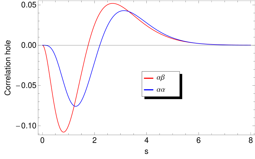
Figure 1: Shape of the approximate correlation holes defined in Eqs 16 and 17. The functions illustrated on the graph are $h_{\mathrm{C}}^{\alpha\beta,1}$ and $h_{\mathrm{C}}^{\alpha\alpha,1}$ multiplied by $4\pi s^{2}$. The functions are evaluated at $r_{\mathrm{s}}=1$ in the spin-compensated HEG limit. Atomic units are used.

The form of correlation holes given in Eq. (16) and Eq. (17) has been derived from observation of system-averaged correlation holes (correlation intracules) in simple systems dominated by dynamical correlation. Qualitatively, the shape of our model correlation hole is similar to correlation intracules in He,Sarsa, Gálvez, and Buendia (1998) Ne,Sarsa, Gálvez, and Buendia (1998) and H2Hollett, McKemmish, and Gill (2011) near the equilibrium bond length. We note that there is a qualitative discrepancy between our approximate correlation hole and the accurate one for systems like LiSarsa, Gálvez, and Buendia (1998) or Be.Sarsa, Gálvez, and Buendia (1998) These systems are characterized by a significant contribution of static correlation. However, there is a substantial cancellation between exchange and correlation holes in systems of this type.

The cusp conditions for same-spin and opposite-spin exchange-correlation holesRajagopal, Kimball, and Banerjee (1978) considerably restrict the short-range expansionBecke (1988b) of $h_{\mathrm{XC}\lambda}^{\alpha\beta}$ and $h_{\mathrm{XC}\lambda}^{\alpha\alpha}$:

$$h_{\mathrm{XC}\lambda}^{\alpha\beta}(\mathbf{r}_{1},s) =(B_{\alpha\beta}-\rho_{\beta})+\lambda B_{\alpha\beta}s+\ldots,$$ (18)

$$h_{\mathrm{XC}\lambda}^{\alpha\alpha}(\mathbf{r}_{1},s) =-\rho_{\alpha}+(B_{\alpha\alpha}-\frac{1}{6}\nabla^{2}\rho_{\alpha})s^{2}+\frac{\lambda}{2}B_{\alpha\alpha}s^{3}+\ldots$$ (19)

Eq. (10) together with Eq. (18), Eq. (19), and the expansion of spherically-averaged exact exchange hole valid at zero current density,Becke (1988b); Lee and Parr (1987); Becke (1996)

$$h_{\mathrm{X}}^{\alpha\alpha}(\mathbf{r}_{1},s)=-\rho_{\alpha}-\frac{1}{6}\left[\nabla^{2}\rho_{\alpha}-2\tau_{\alpha}+\frac{1}{2}\frac{(\nabla\rho_{\alpha})^{2}}{\rho_{\alpha}}\right]s^{2}+\ldots,$$ (20)

yields short-range expansions of correlation holes:Becke (1988b)

$$h_{\mathrm{C}\lambda}^{\alpha\beta}(\mathbf{r}_{1},s) =(B_{\alpha\beta}-\rho_{\beta})+\lambda B_{\alpha\beta}s+\ldots,$$ (21)

$$h_{\mathrm{C}\lambda}^{\alpha\alpha}(\mathbf{r}_{1},s) =\left(B_{\alpha\alpha}-\frac{1}{3}D_{\alpha}\right)s^{2}+\frac{\lambda}{2}B_{\alpha\alpha}s^{3}+\ldots$$ (22)

$D_{\alpha}$ is always non-negative and vanishes for single orbital densities:

$$D_{\alpha}=\tau_{\alpha}-\frac{|\nabla\rho_{\alpha}|^{2}}{4\rho_{\alpha}},$$ (23)

where $\tau_{\alpha}$ is essentially the density of noninteracting kinetic energy

$$\tau_{\alpha}=\sum_{i}^{N_{\alpha}}|\nabla\psi_{i\alpha}|^{2}.$$ (24)

We will adjust the unknown functions $B_{\alpha\beta}$ and $B_{\alpha\alpha}$ in Eq. (18) and Eq. (19) to recover short range expansion of spin-resolved pair distribution function of the HEG developed by Gori-Giorgi and Perdew.Gori-Giorgi and Perdew (2001) The pair distribution function represents the solution of the Overhauser model.Overhauser (1995) $B_{\alpha\alpha}$ will be further modified to eliminate self-interaction error of the correlation functional. We leave the on-top value of the correlation hole (determined solely by $B_{\alpha\beta}$) unchanged by inhomogeneity corrections because it is well-transferable from the HEG to real systems.Burke, Perdew, and Ernzerhof (1998) For the discussion of the quality of the HEG on-top hole density see the work of Burke, Perdew, and Ernzerhof (1998).

Comparison of homogeneous density limit of Eq. (18) and Eq. (19) with short-range expansions of the spin-resolved HEG pair distribution functionGori-Giorgi and Perdew (2001) yields

$$\begin{split}B_{\alpha\beta}(\rho_{\alpha},\rho_{\beta},\lambda)&=\rho_{\beta}\left(1+0.0207\lambda r_{\mathrm{s}}^{\alpha\beta}+0.08193(\lambda r_{\mathrm{s}}^{\alpha\beta})^{2}\right.\\ &\left.-0.01277(\lambda r_{\mathrm{s}}^{\alpha\beta})^{3}+0.001859(\lambda r_{\mathrm{s}}^{\alpha\beta})^{4}\right)\exp(-0.7524\lambda r_{\mathrm{s}}^{\alpha\beta}),\end{split}$$ (25)

$$\begin{split}B_{\alpha\alpha}^{\mathrm{HEG}}(\rho_{\alpha},\lambda)&=\frac{D_{\alpha}^{\mathrm{HEG}}}{3}\left(1-0.01624\lambda r_{\mathrm{s}}^{\alpha\alpha}+0.00264(\lambda r_{\mathrm{s}}^{\alpha\alpha})^{2}\right)\\ &\times\exp(-0.5566\lambda r_{\mathrm{s}}^{\alpha\alpha}),\end{split}$$ (26)

where $r_{\mathrm{s}}^{\alpha\alpha}$ and $r_{\mathrm{s}}^{\alpha\beta}$ introduce the dependence on electronic spin densities,

$$r_{\mathrm{s}}^{\alpha\alpha} =\frac{\left(3/\pi\right)^{1/3}}{2\rho_{\alpha}^{1/3}}$$ (27)

$$r_{\mathrm{s}}^{\alpha\beta} =\frac{\left(3/\pi\right)^{1/3}}{\rho_{\alpha}^{1/3}+\rho_{\beta}^{1/3}}$$ (28)

and each of them reduces to the Seitz radius

$$r_{\mathrm{s}}=\left(\frac{3}{4\pi\rho}\right)^{1/3},$$ (29)

for spin-compensated systems. The formulae (25) and (26) respect the exact high-density expansion derived by Rassolov, Pople, and Ratner (2000). The HEG limit of parameter (23) in (26) readsBecke (1988b)

$$D^{\mathrm{HEG}}_{\alpha}=\frac{3}{5}(6\pi^{2})^{2/3}\rho_{\alpha}^{5/3}.$$ (30)

We substitute $D^{\mathrm{HEG}}_{\alpha}$ in Eq. (26) for $D_{\alpha}$ of Eq. (23) to get $B_{\alpha\alpha}$:

$$\begin{split}B_{\alpha\alpha}(\rho_{\alpha},|\nabla\rho_{\alpha}|,\tau_{\alpha},\lambda)&=\frac{D_{\alpha}}{3}\left(1-0.01624\lambda r_{\mathrm{s}}^{\alpha\alpha}+0.00264(\lambda r_{\mathrm{s}}^{\alpha\alpha})^{2}\right)\\ &\times\exp(-0.5566\lambda r_{\mathrm{s}}^{\alpha\alpha}).\end{split}$$ (31)

Such choice of the $B_{\alpha\alpha}$ function leads to vanishing parallel spin correlation contribution for single orbital densities. In that sense no correlation self-interaction error is present.

Restricting undetermined coefficients in Eq. (16) and Eq. (17) to yield short-range expansions of Eq. (21) and Eq. (22), respectively, gives

$$a_{\alpha\beta} =B_{\alpha\beta}-\rho_{\beta},$$ (32)

$$b_{\alpha\beta} =\lambda B_{\alpha\beta}+d_{\alpha\beta}a_{\alpha\beta}.$$ (33)

Correct shape of $h_{\mathrm{C}\lambda}^{\alpha\beta}$ can be ensured requiring that the function satisfies the appropriate sum rule,

$$4\pi\int_{0}^{\infty}h_{\mathrm{C}\lambda}^{\alpha\beta}(\mathbf{r}_{1},s)s^{2}\mathrm{d}s=0.$$ (34)

Consequently, coefficient $c_{\alpha\beta}$ is fixed for Eq. (34) to hold for all densities:

$$c_{\alpha\beta}=-\frac{1}{12}(a_{\alpha\beta}d_{\alpha\beta}^{2}+3b_{\alpha\beta}d_{\alpha\beta}).$$ (35)

Analogously,

$$a_{\alpha\alpha} =B_{\alpha\alpha}-\frac{D_{\alpha}}{3},$$ (36)

$$b_{\alpha\alpha} =\frac{\lambda}{2}B_{\alpha\alpha}+a_{\alpha\alpha}d_{\alpha\alpha},$$ (37)

$$c_{\alpha\alpha} =-\frac{1}{30}(a_{\alpha\alpha}d_{\alpha\alpha}^{2}+5b_{\alpha\alpha}d_{\alpha\alpha}).$$ (38)

With all but $d_{\alpha\beta}$ and $d_{\alpha\alpha}$ coefficients determined, spin resolved contributions to $V_{\mathrm{C}}^{\lambda}$,

$$V_{\mathrm{C}}^{\sigma\sigma^{\prime},\lambda}=\frac{1}{2}\int\mathrm{d}^{3}\mathbf{r}_{1}\int_{0}^{\infty}\frac{\rho_{\sigma}h_{\mathrm{C}\lambda}^{\sigma\sigma^{\prime}}(\mathbf{r}_{1},s)}{s}4\pi s^{2}\mathrm{d}s,$$ (39)

can now be given as:

$$V_{\mathrm{C}}^{\alpha\beta,\lambda} =\int\mathrm{d}^{3}\mathbf{r}_{1}\rho_{\alpha}\pi\frac{b_{\alpha\beta}+a_{\alpha\beta}d_{\alpha\beta}}{d_{\alpha\beta}^{3}},$$ (40)

$$V_{\mathrm{C}}^{\alpha\alpha,\lambda} =\int\mathrm{d}^{3}\mathbf{r}_{1}\rho_{\alpha}\pi\frac{8b_{\alpha\alpha}+4a_{\alpha\alpha}d_{\alpha\alpha}}{d_{\alpha\alpha}^{5}}.$$ (41)

Several requisites for the exact exchange-correlation functional were derived using uniform coordinate scaling technique,Levy (1991); Levy and Perdew (1985) i.e. by applying uniformly scaled density

$$\rho_{\kappa}(\mathbf{r}_{1})=\kappa^{3}\rho(\kappa\mathbf{r}_{1}).$$ (42)

These relations are particularly valuable because they hold for arbitrary $N$-electron densities. A density-scaling identity proved by Levy,Levy (1991)

$$h_{\mathrm{C}\lambda}^{\sigma\sigma^{\prime}}(\rho;\mathbf{r}_{1},s)=\lambda^{3}h_{\mathrm{C}\lambda^{\prime}=1}^{\sigma\sigma^{\prime}}(\rho_{1/\lambda};\lambda\mathbf{r}_{1},\lambda s),$$ (43)

constrains the set of admissible forms of $d_{\alpha\beta}$ and $d_{\alpha\alpha}$. Eq. (43) implies that

$$d_{\sigma\sigma^{\prime}}(\rho,|\nabla\rho|,\lambda)=\lambda d_{\sigma\sigma^{\prime}}\left(\frac{\rho}{\lambda^{3}},\frac{|\nabla\rho|}{\lambda^{4}},1\right).$$ (44)

We propose the following simple function which satisfies the scaling condition:

$$d_{\sigma\sigma^{\prime}}=\frac{F_{\sigma\sigma^{\prime}}}{r_{\mathrm{s}}^{\sigma\sigma^{\prime}}}+\frac{G}{r_{\mathrm{s}}}\frac{\nabla\rho\cdot\nabla\rho}{\rho^{8/3}}.$$ (45)

As Eq. (45) is independent of $\lambda$, the coupling-constant integration of Eq. (7) can be done analytically. The values of $F_{\alpha\beta}$ and $F_{\alpha\alpha}$ were determined by least-squares fit of the HEG limit of $V_{\mathrm{C}}^{\alpha\beta,\lambda=1}$ and $V_{\mathrm{C}}^{\alpha\alpha,\lambda=1}$ to the reference values.Gori-Giorgi, Sacchetti, and Bachelet (2000) Opposite-spin and parallel-spin components were fit independently. Reference values of $V_{\mathrm{C}}^{\sigma\sigma^{\prime},\lambda=1}$ for the HEG were obtained by Gori-Giorgi et al.Gori-Giorgi, Sacchetti, and Bachelet (2000) by integrating pair correlation functions from quantum Monte Carlo simulation.Ortiz, Harris, and Ballone (1999) Our estimates of $V_{\mathrm{C}}^{\alpha\beta,\lambda=1}$ and $V_{\mathrm{C}}^{\alpha\alpha,\lambda=1}$ were optimized to recover the reference values for spin-compensated system at metallic densities ($r_{\mathrm{s}}=1,2,3,\ldots,10$). The resulting parameters are $F_{\alpha\beta}=2.1070$ and $F_{\alpha\alpha}=2.6422$. The corresponding mean absolute percentage errors (MAPE) of opposite-spin and parallel-spin components are $5.0\%$ and $12.0\%$, respectively. The MAPE of total $V_{\mathrm{C}}^{\lambda=1}$ is equal to $4.6\%$. See Fig. 2 for comparison of our fit to the reference values. At high densities ($r_{\mathrm{s}}<1$) our model does not reduce to the accurate correlation functional for the HEG as it does not account for the logarithmic divergence of the correlation energy density for $r_{\mathrm{s}}\rightarrow 0$.Gell-Mann and Brueckner (1957) This is, however, a peculiarity of the HEG that is not present in finite molecular systems.

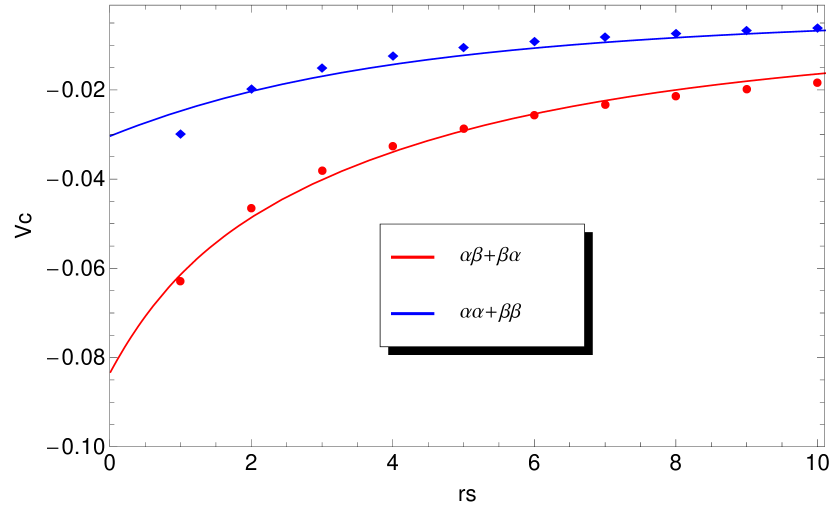
Figure 2: Comparison of the approximate $V_{\mathrm{C}}^{\sigma\sigma^{\prime},\lambda=1}$ energies in the HEG limit with reference Monte Carlo data.Gori-Giorgi, Sacchetti, and Bachelet (2000) Solid lines refer to Eqs 40 and 41. Circles and diamonds represent reference values. The cause of discrepancy at low $r_{\mathrm{s}}$ (high densities) is discussed in the main text. Atomic units are used.

We supply our SL correlation functional with the DFT-D3 dispersion correction of Grimme et al. (2010), which contributes damped terms of the multipole expansion of the dispersion energy. The adjustment of the SL part to harmonize with the NL correction is accomplished by optimization of the $G$ parameter, see (45). The $G$ parameter can be adjusted freely, without interfering with any of the above-mentioned physical and formal constraints. In particular, it does not alter the first two terms in the short-range spatial Taylor expansion of the correlation holes. The value of $G$ can be chosen so that the correlation contributions described by SL and NL parts do not overlap. As $G\rightarrow 0$, our SL correlation model reduces to the correlation of the HEG with self-interaction removed from parallel-spin part. Our numerical results show that this leads to a systematic overestimation of intermolecular interactions. On the other hand, when $G\rightarrow\infty$, the SL correlation vanishes, and the SL functional reduces to an exchange-only approximation (without adding the dispersion correction). Provided that the exchange functional is free from artificial binding, the interaction energies should be underestimated in this limit. Between these two limits lays the optimal $G$, which corresponds to an interaction curve slightly shallower than the real one, for the addition of the negative dispersion term should move the interaction energy towards the accurate value.

The $G$ parameter of Eq. 45 and the two empirical parameters present in DFT-D3 dispersion correction, $s_{r,6}$ and $s_{8}$, (see Eqs. 3 and 4 in Ref. 10) were chosen to optimize mean absolute percentage error of binding energies in S22 set of non-covalently bound complexes.Jurecka et al. (2006) The numerical optimization has been carried out with the constraint that the dispersion-free energy cannot fall below the reference total interaction energy. During the optimization process, self-consistent KS calculations in aug-cc-pVTZ basis set were performed using the molecular structures published in Ref. 66. Reference interaction energies were taken from Ref. 67. The resulting optimal values are $G=0.096240$, $s_{r,6}=1.1882$, and $s_{8}=0.65228$. The interaction energies in S22 set are presented in Table 2.

III Implementation

The expression for the correlation energy is obtained after inserting Eq. (40) and Eq. (41) into Eq. (7) and integrating with respect to $\lambda$. Below we present $E_{\mathrm{C}}$ in a form convenient for implementation.

$$E_{\mathrm{C}} =E_{\mathrm{C}}^{\alpha\beta}+E_{\mathrm{C}}^{\beta\alpha}+E_{\mathrm{C}}^{\alpha\alpha}+E_{\mathrm{C}}^{\beta\beta},$$ (46)

$$E_{\mathrm{C}}^{\alpha\beta} =\int_{0}^{1}V_{\mathrm{C}}^{\alpha\beta,\lambda}\mathrm{d}\lambda=\int\mathrm{d}^{3}\mathbf{r}_{1}\rho_{\alpha}\pi\frac{\mathcal{B}_{\alpha\beta}+\mathcal{A}_{\alpha\beta}d_{\alpha\beta}}{d_{\alpha\beta}^{3}},$$ (47)

$$E_{\mathrm{C}}^{\alpha\alpha} =\int_{0}^{1}V_{\mathrm{C}}^{\alpha\alpha,\lambda}\mathrm{d}\lambda=\int\mathrm{d}^{3}\mathbf{r}_{1}\rho_{\alpha}\pi\frac{8\mathcal{B}_{\alpha\alpha}+4\mathcal{A}_{\alpha\alpha}d_{\alpha\alpha}}{d_{\alpha\alpha}^{5}},$$ (48)

$$\mathcal{A}_{\alpha\beta} =\frac{\rho_{\beta}}{r_{\mathrm{s}}^{\alpha\beta}}\left[\left(-P_{0}+\sum_{k=1}^{4}P_{k}(r_{\mathrm{s}}^{\alpha\beta})^{k}\right)\exp\left(-P_{5}r_{\mathrm{s}}^{\alpha\beta}\right)+P_{0}\right]-\rho_{\beta}$$ (49)

$$\mathcal{B}_{\alpha\beta} =\frac{\rho_{\beta}}{(r_{\mathrm{s}}^{\alpha\beta})^{2}}\left[\left(-Q_{0}+\sum_{k=1}^{5}Q_{k}(r_{\mathrm{s}}^{\alpha\beta})^{k}\right)\exp\left(-Q_{6}r_{\mathrm{s}}^{\alpha\beta}\right)+Q_{0}\right]+d_{\alpha\beta}\mathcal{A}_{\alpha\beta}$$ (50)

$$\mathcal{A}_{\alpha\alpha} =\frac{D_{\alpha}}{3r_{\mathrm{s}}^{\alpha\alpha}}\left[\left(-R_{0}+\sum_{k=1}^{2}R_{k}(r_{\mathrm{s}}^{\alpha\alpha})^{k}\right)\exp\left(-R_{3}r_{\mathrm{s}}^{\alpha\alpha}\right)+R_{0}\right]-\frac{D_{\alpha}}{3}$$ (51)

$$\mathcal{B}_{\alpha\alpha} =\frac{D_{\alpha}}{6(r_{\mathrm{s}}^{\alpha\alpha})^{2}}\left[\left(-S_{0}+\sum_{k=1}^{3}S_{k}(r_{\mathrm{s}}^{\alpha\alpha})^{k}\right)\exp\left(-S_{4}r_{\mathrm{s}}^{\alpha\alpha}\right)+S_{0}\right]+d_{\alpha\alpha}\mathcal{A}_{\alpha\alpha}$$ (52)

Note that $E_{\mathrm{C}}^{\alpha\beta}=E_{\mathrm{C}}^{\beta\alpha}$. The formula for $E_{\mathrm{C}}^{\beta\beta}$ can be obtained by substitution of spin indices in $E_{\mathrm{C}}^{\alpha\alpha}$. The values of the numerical constants appearing in Eqs. 49–52 are listed in Table 1. The following functions: $D_{\alpha}$, $r_{\mathrm{s}}^{\alpha\alpha}$, and $r_{\mathrm{s}}^{\alpha\beta}$ are defined in Eqs 23, 27, 28, respectively. The $d_{\sigma\sigma^{\prime}}$ function, defined in Eq. 45, is parametrized as follows:

$$d_{\alpha\beta} =\frac{2.1070}{r_{\mathrm{s}}^{\alpha\beta}}+\frac{0.096240}{r_{\mathrm{s}}}\frac{\nabla\rho\cdot\nabla\rho}{\rho^{8/3}},$$ (53)

$$d_{\alpha\alpha} =\frac{2.6422}{r_{\mathrm{s}}^{\alpha\alpha}}+\frac{0.096240}{r_{\mathrm{s}}}\frac{\nabla\rho\cdot\nabla\rho}{\rho^{8/3}}.$$ (54)

The parameters appearing in DFT-D3 correctionGrimme et al. (2010) are $s_{r,6}=1.1882$ and $s_{8}=0.65228$. Fortran code for numerical evaluation of the correlation energy and its derivatives, together with the corresponding Mathematicamat (2008) notebook, can be obtained from the authors by e-mail or from their webpage. The calculations presented in this work were done using GAMESS program.Schmidt et al. (1993); Gordon and Schmidt (2005)

Table 1: Ab initio numerical constants appearing in Eqs 49–52

k	$P_{k}$	$Q_{k}$	$R_{k}$	$S_{k}$
$0$	$1.696$	$3.356$	$1.775$	$3.205$
$1$	$-0.2763$	$-2.525$	$0.01213$	$-1.784$
$2$	$-0.09359$	$-0.4500$	$-4.743\times 10^{-3}$	$3.613\times 10^{-3}$
$3$	$3.837\times 10^{-3}$	$-0.1060$	$0.5566$	$-4.743\times 10^{-3}$
$4$	$-2.471\times 10^{-3}$	$5.532\times 10^{-4}$		$0.5566$
$5$	$0.7524$	$-2.471\times 10^{-3}$
$6$		$0.7524$

IV Discussion

Similar strategy for designing a correlation functional, i.e., constructing a real-space model for a spin-resolved correlation hole, was originally proposed by Rajagopal, Kimball, and Banerjee (1978) with the first application by Becke (1988b), followed by the works of Proynov and Salahub (1994) and Tsuneda, Suzumura, and Hirao (1999). A central role in those methods is played by correlation length, a function completely determining both short- and long-range behavior of the correlation holes present in those models. Our approach has more degrees of freedom, as the short-range behavior of $h_{\mathrm{C}\lambda}^{\sigma\sigma^{\prime}}$ is decoupled from the choice of the $d_{\sigma\sigma^{\prime}}$ function which controls its decay. This flexibility allows us to adjust $d_{\sigma\sigma^{\prime}}$ to match a specific NL correction without sacrificing the short-range correlation that can be accurately represented by an SL functional.

The ultimate goal is to develop a general-purpose functional that not only yields satisfactory results for the dispersion interactions, but also performs not worse than the existing approximations in predicting other properties of chemical interest. To do so, the inclusion of the NL constituent and the accompanying adjustment of the SL part should not affect any of the energetically important constraints already satisfied by the meta-GGA rung functionals.Perdew et al. (2005) Among the formal constraints, the most fundamental one is the non-positivity condition,

$$V_{\mathrm{C}}^{\sigma\sigma^{\prime},\lambda}\left[\rho\right]\leq 0,$$ (55)

which is obeyed by our model for every spin-density. Similarly, the scaling conditions formulated by Levy,Levy (1991) e.g.,

$$\lim_{\kappa\rightarrow 0}\frac{E_{\mathrm{C}}\left[\rho_{\kappa}\right]}{\kappa} =\sum_{\sigma\sigma^{\prime}}\lim_{\lambda\rightarrow\infty}V_{\mathrm{C}}^{\sigma\sigma^{\prime},\lambda}\left[\rho\right]>-\infty,$$ (56)

$$\frac{\partial V_{\mathrm{C}}^{\sigma\sigma^{\prime},\lambda}\left[\rho\right]}{\partial\lambda} \leq 0,$$ (57)

together with the high-density limit of the correlation functional,Levy (1989)

$$\lim_{\kappa\rightarrow\infty}E_{\mathrm{C}}\left[\rho_{\kappa}\right]>-\infty,$$ (58)

are satisfied. A failure to satisfy condition (58) may contribute to overbinding of molecules.Levy (1991)

In addition to conditions (55)–(58), our approximation satisfies a constraint which has a direct connection to the prediction of interaction energies. It was observed by Kamiya, Tsuneda, and Hirao (2002) that if an SL functional yields nonzero contributions to the correlation in the tail of the density, then adding an NL correction may lead to a severe overbinding.Kamiya, Tsuneda, and Hirao (2002) In the tail of electronic density, where the reduced gradient is large, the $d_{\sigma\sigma^{\prime}}$ function of Eq. (45) goes to infinity, thus our SL correlation correctly vanishes.

The correlation self-interaction error is corrected using $\tau_{\sigma}$ variable (the kinetic energy density), see Eq. (31), similarly to other meta-GGA correlation functionalsBecke (1988b); Perdew et al. (1999); Zhao, Schultz, and Truhlar (2006). As a result, in our model the parallel-spin correlation vanishes for single-orbital spin-compensated densities, and the total correlation energy is zero for hydrogen atom.

The above-mentioned constraints are merely formal prerequisites for a high-quality approximation to $E_{\mathrm{C}}$. A decent approximate model should also capture the physics of molecular systems. Our model reflects the following physical properties:

1. Short-range electronic correlation is modeled by an expression borrowed from the homogeneous electron gas, which is also appropriate for real systems.Burke, Perdew, and Langreth (1994); Burke, Perdew, and Ernzerhof (1998); Henderson and Bartlett (2004); Cancio, Fong, and Nelson (2000) (See Eqs 25, 26, and 31.) To the best of our knowledge, we present the first beyond-LDA functional which incorporates analytic representation of the short-range correlation function of the HEG developed by Gori-Giorgi and Perdew (2001).

2. Long-range behavior of the correlation hole is governed by $d_{\sigma\sigma^{\prime}}$ function (see Eqs 16, 17, and 45), which depends on both density and its gradient at a reference point. This function accounts for damping effect of density inhomogeneity ($\nabla\rho_{\sigma}$) on the correlation hole. Furthermore, the $d_{\sigma\sigma^{\prime}}$ function contains a free parameter, $G$. It is used in tuning the spatial range separation of the correlation hole to properly blend with the long-range correlation correction.

3. Our model closely approximates the exact correlation in the HEG regime at metallic densities. (See also the discussion below Eq. (45).)

To make our concept of stitching SL and NL correlation more transparent, we briefly discuss it in the context of range-separated approach of Kohn, Meir, and Makarov (1998). It is possible to solve the dispersion problem within DFT by partitioning the interelectron repulsion, $1/r$, into short-range part, $\exp\left(-\mu r\right)/r$, and its long-range complement.Kohn, Meir, and Makarov (1998) ($\mu$ is a constant.) Both short-range exchange and correlation are then treated at (semi)local level, and the contributions originating from the long-range interaction are approximated by a formula that is consistent with the Casimir-Polder expression in the asymptotic region. Our treatment follows the same general idea. The difference is as follows: the exponential factor that damps the interelectronic interaction, $\exp\left(-\mu r\right)$, is replaced by the $\exp\left(-d_{\sigma\sigma^{\prime}}r\right)$ function of Eqs 16–17 which damps the short range expansion of the approximate correlation holes. Thus, the $\mu$ constant is generalized into $d_{\sigma\sigma^{\prime}}$ function, which depends on density and its gradient at a reference point.

V Numerical results

Our aim was to validate the correlation functional presented in this work, preferably without the interference from the errors of an exchange approximation. Therefore, we decided to perform calculations using our correlation combined with full HF-like exchange, and to compare it with other DFAs involving full HF-like exchange. Although a general-purpose approximation cannot be formed by combining semilocal DFT correlation with full exact exchange, it is a demanding and useful test for a correlation functional. If the correlation functional performs well with large portion of the exact exchange, then there is much room for adjusting the exchange part of a global hybrid or a range-separated hybrid exchange-correlation functional.

All DFT and HF calculations presented below were performed in aug-cc-pVTZ basis. All energies are obtained from self-consistent calculations. Table 2 contains interaction energies for S22 set of molecules.Jurecka et al. (2006) The reference energies, $E_{\mathrm{ref}}$, are taken from Ref. 67. $E_{\mathrm{int}}$ denotes interaction energy calculated using the correlation functional described in this work combined with $100\%$ HF-like exchange and DFT-D3 correction. All energies, as well as mean signed errors (MSE) and mean unsigned errors (MUE) are given in kcal/mol. Mean absolute percentage errors (MAPE) are given in percent. Our results (MUE=$0.46$ kcal/mol) compare rather favorably to the other methods utilizing full HF-like exchange, VV09Vydrov and Van Voorhis (2010b) (MUE=$0.90$ kcal/mol), M06HFZhao and Truhlar (2008); Goerigk and Grimme (2011) (MUE=$0.62$ kcal/mol), and M06HF-D3Zhao and Truhlar (2008); Goerigk and Grimme (2011) (MUE=$0.84$ kcal/mol). The dispersion-free interaction energies are always significantly below the values that would be obtained if the dispersion term as defined in SAPT was subtracted, see supplementary information in Ref. 18 and Ref. 82. This fact suggests that in our model, at equilibrium distances, a large fraction of the dispersion interaction is treated as short-range and accounted for by the SL functional.

We further evaluate the performance of our approximation on the set of systems from nonbonded interaction database of Zhao and Truhlar.Zhao and Truhlar (2005a, b) This database gathers interacting dimers in subsets according to the dominant character of the interaction: dispersion-dominated (WI7/05 and PPS5/05 subsets), dipole interaction (DI6/04 subset), hydrogen-bonded (HB6/04), and charge transfer (CT7/04). The results are presented in Tables 3, 4, 5, 6, and 7, respectively. The reference energies ($E_{\mathrm{ref}}$) are calculated at CCSD(T)/mb-aug-cc-pVTZ level, see Ref. 18. We compare our approximation ($E_{\mathrm{int}}$) with M06HF functionalZhao and Truhlar (2008) ($E_{\mathrm{M06HF}}$) which combines empirically-parametrized meta-GGA correlation with full HF-like exchange. As expected, our model predicts interaction energies more accurately in cases where the dispersion interaction dominates, see Tables 3 and 4. In case of hydrogen bonded complexes, Table 6, MAPE of either functional is close to $5\%$. Larger errors are present in DI6/04 and CT7/04 subsets. Although our approximation performs better that M06HF in case of DI6/04 dimers, the error is rather large. In this case, as is seen in Table 5, both functionals underestimate the interaction strength and their errors are correlated. This fact suggests that the contribution coming from full HF-like exchange is too repulsive, which cannot be counterbalanced by semilocal DFT correlation. Both functionals display largest errors in charge-transfer complexes. Our approximation underestimates interaction for every CT complex. This behavior to a large degree results from huge errors of the HF theory itself, see $E_{\mathrm{HF}}$ column in Table 7. As explained by Cohen, Mori-Sánchez, and Yang (2012) this problem can be traced to the localization error of the HF theory, which makes electrons excessively localized on the monomers. This error manifests itself as a concave curve of energy vs. fractional number of electrons, $E(N)$.Cohen, Mori-Sánchez, and Yang (2012) It is also known that pure semilocal DFT approximations give convex $E(N)$.Cohen, Mori-Sánchez, and Yang (2012) See Ref. 82 for the relevant discussion of NH3…ClF dimer. Therefore, adding some amount of semilocal exchange to our approximation should make the $E(N)$ dependence more linear and make the exchange contribution in CT interactions less repulsive, the step which will be undertaken in the future.

Table 2: Interaction energies in S22 set (kcal/mol).

Dimer	$E_{\mathrm{ref}}$	$E_{\mathrm{int}}$	$E_{\mathrm{dispfree}}$
Hydrogen-bonded
(NH3)2	-3.145	-2.75	-2.17
(H2O)2	-5.004	-4.86	-4.41
Formic acid dimer	-18.751	-20.17	-18.75
Formamide dimer	-16.063	-16.46	-14.86
Uracil dimer planar ($C_{2h}$)	-20.643	-21.30	-19.10
2-pyridone $\cdot$ 2-aminopyridine	-16.938	-16.33	-13.67
Adenine $\cdot$ thymine WC	-16.554	-16.15	-13.24
MSE	-0.13
MUE	0.58
MAPE	5.0
Predominant dispersion
(CH4)2	-0.529	-0.60	0.14
(C2H4)2	-1.482	-1.52	-0.15
Benzene $\cdot$ CH4	-1.448	-1.45	0.10
Benzene dimer parallel-displaced ($C_{2h}$)	-2.655	-1.76	2.55
Pyrazine dimer	-4.256	-3.36	0.99
Uracil dimer stacked ($C_{2}$)	-9.783	-9.97	-3.63
Indole $\cdot$ benzene stacked	-4.523	-3.25	2.73
Adenine $\cdot$ thymine stacked	-11.857	-11.63	-3.10
MSE	0.37
MUE	0.45
MAPE	13
Mixed interaction
Ethene $\cdot$ ethyne	-1.503	-1.63	-0.91
Benzene H2O	-3.280	-3.78	-2.19
Benzene NH3	-2.319	-2.55	-0.92
Benzene HCN	-4.540	-5.68	-4.02
Benzene dimer T-shaped ($C_{2v}$)	-2.717	-2.72	-0.18
Indole $\cdot$ benzene T-shaped	-5.627	-5.89	-2.45
Phenol dimer	-7.097	-6.87	-3.96
MSE	-0.29
MUE	0.36
MAPE	9.5
MSE (total)	0.002
MUE (total)	0.46
MAPE (total)	9.3

Table 3: Interaction energies in WI7/05 set (kcal/mol).

Dimer	$E_{\mathrm{ref}}$	$E_{\mathrm{int}}$	$E_{\mathrm{M06HF}}$
He…Ne	-0.041	-0.037	-0.13
He…Ar	-0.058	-0.045	-0.085
Ne…Ne	-0.086	-0.064	-0.13
Ne…Ar	-0.13	-0.07	-0.15
CH4…Ne	-0.18	-0.18	-0.20
C6H6…Ne	-0.41	-0.53	-0.66
CH4…CH4	-0.53	-0.59	-0.12
MSE		-0.01	-0.006
MUE		0.04	0.12
MAPE		21	68

Table 4: Interaction energies in PPS5/05 set (kcal/mol).

Dimer	$E_{\mathrm{ref}}$	$E_{\mathrm{int}}$	$E_{\mathrm{M06HF}}$
(C2H2)2	-1.36	-1.47	-1.06
(C2H4)2	-1.44	-1.52	-0.95
Sandwich (C6H6)2	-1.65	-0.95	0.48
T-shaped (C6H6)2	-2.63	-2.78	-1.95
Displaced (C6H6)2	-2.59	-2.06	-0.94
MSE		0.18	1.0
MUE		0.31	1.0
MAPE		16	55

Table 5: Interaction energies in DI6/04 set (kcal/mol).

Dimer	$E_{\mathrm{ref}}$	$E_{\mathrm{int}}$	$E_{\mathrm{M06HF}}$
H2S…H2S	-1.62	-1.20	-0.82
HCl…HCl	-1.91	-1.40	-0.99
HCl…H2S	-3.26	-2.74	-2.48
CH3Cl…HCl	-3.39	-2.77	-2.72
CH3SH…HCN	-3.58	-3.70	-3.50
CH3SH…HCl	-4.74	-4.13	-4.27
MSE		0.43	0.62
MUE		0.47	0.62
MAPE		17	26

Table 6: Interaction energies in HB6/04 set (kcal/mol).

Dimer	$E_{\mathrm{ref}}$	$E_{\mathrm{int}}$	$E_{\mathrm{M06HF}}$
NH3…NH3	-3.09	-2.82	-2.53
HF…HF	-4.49	-4.63	-4.27
H2O…H2O	-4.91	-4.90	-4.72
NH3…H2O	-6.38	-6.28	-6.35
(HCONH2)2	-15.41	-16.39	-15.72
(HCOOH)2	-17.60	-19.57	-19.33
MSE		-0.45	0.28
MUE		0.58	0.30
MAPE		5.2	4.6

Table 7: Interaction energies CT7/04 (kcal/mol).

Dimer	$E_{\mathrm{ref}}$	$E_{\mathrm{int}}$	$E_{\mathrm{M06HF}}$	$E_{\mathrm{HF}}$
C2H4…F2	-1.06	-0.33	-0.67	0.71
NH3…F2	-1.80	-0.74	-0.90	0.19
C2H2…ClF	-3.79	-2.98	-4.18	-0.16
HCN…ClF	-4.80	-3.70	-4.02	-2.10
NH3…Cl2	-4.85	-3.50	-4.00	-1.12
H2O…ClF	-5.20	-4.69	-5.26	-2.91
NH3…ClF	-11.17	-10.53	-11.92	-5.49
MSE		0.89	0.24
MUE		0.89	0.59
MAPE		31	20

VI Conclusions

This paper presents a novel form of an SL correlation functional belonging to the meta-GGA rung that may be combined in an optimal way with the dispersion interaction component, either in the DFT+D manner or by incorporating a nonlocal potential. The important feature is that it is based on the first principles, in the form of a number of physical constraints imposed during the derivation. With minimal empiricism, our approximation is adjusted to a desired long-range dispersion correction by optimizing only a single empirical parameter. The parameter has a clear physical meaning: it governs the decay of the approximate correlation hole. Consequently, the correlation hole vanishes exponentially at large inter-electronic distances, which prevents double counting of the electron correlation effect that is already included when adding the long-range dispersion correction. An important and unique facet of our functional is that the adjustment of the empirical range-separation parameter has not relaxed any of the physical constraints on which our model is based. The electron correlation is approximated by utilizing several numerical and analytical results of the HEG model. Most importantly, the HEG approximation to the short-range part of the correlation hole is rigorously conserved for arbitrary systems (only the self-interaction pertinent to the HEG model is removed from the parallel-spin correlation hole).

While our new correlation functional can be combined with any of non-local dispersion models, for preliminary calculations of this paper, we employed the atom pairwise additive DFT-D3 dispersion correction. Given the fact that our correlation functional is combined with 100% HF exchange – far from an optimal choice in general case – the numerical results are very encouraging. For the interaction energies of hydrogen-bonded complexes, the accuracy is on a par with that obtained with the M06HF functional, which is a highly parametrized empirical approximation containing full HF exchange. For dispersion-dominated complexes, the predictions of our model compare favorably with VV09 and M06HF. The results in the subsets of dipole-interaction and charge-transfer complexes are less satisfactory, which is easily explained by the inadequacy of the full HF-like exchange component: indeed, the signed errors correlate with the signed errors of the HF method. Obviously, much improvement may be expected when a more appropriate exchange part will be incorporated. Development of an optimal range-separated hybrid exchange approximation, appropriate for our new correlation functional, as well as implementation of non-local van der Waals correlation functionals are underway in our laboratory.

VII Acknowledgments

This work was supported by the Polish Ministry of Science and Higher Education, Grant N N204 248440, and by the National Science Foundation (US), Grant No. CHE-1152474.

References

- Dobson (2012) J. Dobson, in Fundamentals of Time-Dependent Density Functional Theory, Lecture Notes in Physics, Vol. 837, edited by M. A. Marques, N. T. Maitra, F. M. Nogueira, E. Gross, and A. Rubio (Springer Berlin / Heidelberg, 2012) p. 417.
- Dobson et al. (2005) J. F. Dobson, J. Wang, B. P. Dinte, K. McLennan, and H. M. Le, Int. J. Quant. Chem. 101, 579 (2005).
- Cohen, Mori-Sánchez, and Yang (2012) A. J. Cohen, P. Mori-Sánchez, and W. Yang, Chem. Rev. 112, 289 (2012).
- Dobson and Gould (2012) J. Dobson and T. Gould, J. Phys.: Condens. Matter 24, 073201 (2012).
- Becke and Johnson (2005a) A. Becke and E. Johnson, J. Chem. Phys. 122, 154104 (2005a).
- Becke and Johnson (2005b) A. Becke and E. Johnson, J. Chem. Phys. 123, 154101 (2005b).
- Becke and Johnson (2007) A. Becke and E. Johnson, J. Chem. Phys. 127, 124108 (2007).
- Heßelmann (2009) A. Heßelmann, J. Chem. Phys. 130, 084104 (2009).
- Ángyán (2007) J. Ángyán, J. Chem. Phys. 127, 024108 (2007).
- Grimme et al. (2010) S. Grimme, J. Antony, S. Ehrlich, and H. Krieg, J. Chem. Phys. 132, 154104 (2010).
- Tkatchenko and Scheffler (2009) A. Tkatchenko and M. Scheffler, Phys. Rev. Lett. 102, 073005 (2009).
- Dion et al. (2004) M. Dion, H. Rydberg, E. Schröder, D. Langreth, and B. Lundqvist, Phys. Rev. Lett. 92, 246401 (2004).
- Lee et al. (2010) K. Lee, É. Murray, L. Kong, B. Lundqvist, and D. Langreth, Phys. Rev. B 82, 081101 (2010).
- Vydrov and Van Voorhis (2009a) O. Vydrov and T. Van Voorhis, J. Chem. Phys. 130, 104105 (2009a).
- Vydrov and Van Voorhis (2009b) O. Vydrov and T. Van Voorhis, Phys. Rev. Lett. 103, 63004 (2009b).
- Vydrov and Van Voorhis (2010a) O. Vydrov and T. Van Voorhis, J. Chem. Phys. 133, 244103 (2010a).
- Vydrov and Voorhis (2012) O. Vydrov and T. Voorhis, in Fundamentals of Time-Dependent Density Functional Theory, Lecture Notes in Physics, Vol. 837, edited by M. A. Marques, N. T. Maitra, F. M. Nogueira, E. Gross, and A. Rubio (Springer Berlin / Heidelberg, 2012) pp. 443–456.
- Pernal et al. (2009) K. Pernal, R. Podeszwa, K. Patkowski, and K. Szalewicz, Phys. Rev. Lett. 103, 263201 (2009).
- Rajchel et al. (2010) Ł. Rajchel, P. Żuchowski, M. M. Szcz\textpolhookeśniak, and G. Chałasiński, Chem. Phys. Lett. 486, 160 (2010).
- Kamiya, Tsuneda, and Hirao (2002) M. Kamiya, T. Tsuneda, and K. Hirao, J. Chem. Phys. 117, 6010 (2002).
- Murray, Lee, and Langreth (2009) E. D. Murray, K. Lee, and D. C. Langreth, J. Chem. Theory Comput. 5, 2754 (2009).
- Perdew, Burke, and Ernzerhof (1996) J. Perdew, K. Burke, and M. Ernzerhof, Phys. Rev. Lett. 77, 3865 (1996).
- Becke (1988a) A. D. Becke, Phys. Rev. A 38, 3098 (1988a).
- Perdew and Yue (1986) J. P. Perdew and W. Yue, Phys. Rev. B 33, 8800 (1986).
- Vydrov and Van Voorhis (2010b) O. Vydrov and T. Van Voorhis, J. Chem. Phys. 132, 164113 (2010b).
- Grimme and Ehrlich (2011) S. Grimme and S. Ehrlich, J. Comp. Chem. 32, 1456 (2011).
- Dobson et al. (2002) J. Dobson, K. McLennan, A. Rubio, J. Wang, T. Gould, H. Le, and B. Dinte, Aust. J. Chem. 54, 513 (2002).
- Hesselmann and Jansen (2003) A. Hesselmann and G. Jansen, Chem. Phys. Lett. 367, 778 (2003).
- Misquitta et al. (2005) A. Misquitta, R. Podeszwa, B. Jeziorski, and K. Szalewicz, J. Chem. Phys. 123, 214103 (2005).
- Koide (1976) A. Koide, J. Phys. B 9, 3173 (1976).
- Burcl et al. (1995) R. Burcl, G. Chałasiński, R. Bukowski, and M. M. Szcz\textpolhookeśniak, J. Chem. Phys. 103, 1498 (1995).
- Koide, Meath, and Allnatt (1981) A. Koide, W. J. Meath, and A. Allnatt, Chem. Phys. 58, 105 (1981).
- Burns et al. (2011) L. A. Burns, A. Vazquez-Mayagoitia, B. G. Sumpter, and C. D. Sherrill, J. Chem. Phys. 134, 084107 (2011).
- Goerigk and Grimme (2011) L. Goerigk and S. Grimme, Phys. Chem. Chem. Phys. 13, 6670 (2011).
- Hujo and Grimme (2011) W. Hujo and S. Grimme, J. Chem. Theory Comput. 7, 3866 (2011).
- Vazquez-Mayagoitia et al. (2010) A. Vazquez-Mayagoitia, C. D. Sherrill, E. Apra, and B. G. Sumpter, J. Chem. Theory Comput. 6, 727 (2010).
- Thanthiriwatte et al. (2011) K. S. Thanthiriwatte, E. G. Hohenstein, L. A. Burns, and C. D. Sherrill, J. Chem. Theory Comput. 7, 88 (2011).
- Grimme (2006) S. Grimme, J. Comp. Chem. 27, 1787 (2006).
- Chai and Head-Gordon (2008a) J. Chai and M. Head-Gordon, Phys. Chem. Chem. Phys. 10, 6615 (2008a).
- Chai and Head-Gordon (2008b) J. Chai and M. Head-Gordon, J. Chem. Phys. 128, 084106 (2008b).
- Ruiz, Salahub, and Vela (1996) E. Ruiz, D. Salahub, and A. Vela, J. Phys. Chem. 100, 12265 (1996).
- Sini, Sears, and Bredas (2011) G. Sini, J. S. Sears, and J.-L. Bredas, J. Chem. Theory Comput. 7, 602 (2011).
- Podeszwa et al. (2010) R. Podeszwa, K. Pernal, K. Patkowski, and K. Szalewicz, J. Phys. Chem. Lett. 1, 550 (2010).
- Swart, Solà, and Bickelhaupt (2009) M. Swart, M. Solà, and F. Bickelhaupt, J. Chem. Phys. 131, 094103 (2009).
- Becke (1997) A. D. Becke, J. Chem. Phys. 107, 8554 (1997).
- Levy (1979) M. Levy, PNAS 76, 6062 (1979).
- Hohenberg and Kohn (1964) P. Hohenberg and W. Kohn, Phys. Rev. 136, B864 (1964).
- Kohn and Sham (1965) W. Kohn and L. J. Sham, Phys. Rev. 140, A1133 (1965).
- Levy (1996) M. Levy, in Theoretical and Computational Chemistry, Vol. 4, edited by J. Seminario (Elsevier, 1996).
- Baerends and Gritsenko (1997) E. Baerends and O. Gritsenko, J. Phys. Chem. A 101, 5383 (1997).
- Burke, Perdew, and Ernzerhof (1998) K. Burke, J. Perdew, and M. Ernzerhof, J. Chem. Phys. 109, 3760 (1998).
- Sarsa, Gálvez, and Buendia (1998) A. Sarsa, F. Gálvez, and E. Buendia, J. Chem. Phys. 109, 7075 (1998).
- Hollett, McKemmish, and Gill (2011) J. Hollett, L. McKemmish, and P. Gill, J. Chem. Phys. 134, 224103 (2011).
- Rajagopal, Kimball, and Banerjee (1978) A. Rajagopal, J. Kimball, and M. Banerjee, Phys. Rev. B 18, 2339 (1978).
- Becke (1988b) A. Becke, J. Chem. Phys. 88, 1053 (1988b).
- Lee and Parr (1987) C. Lee and R. Parr, Phys. Rev. A 35, 2377 (1987).
- Becke (1996) A. Becke, Can. J. Chem. 74, 995 (1996).
- Gori-Giorgi and Perdew (2001) P. Gori-Giorgi and J. Perdew, Phys. Rev. B 64, 155102 (2001).
- Overhauser (1995) A. Overhauser, Can. J. Phys. 73, 683 (1995).
- Rassolov, Pople, and Ratner (2000) V. Rassolov, J. Pople, and M. Ratner, Phys. Rev. B 62, 2232 (2000).
- Levy (1991) M. Levy, Phys. Rev. A 43, 4637 (1991).
- Levy and Perdew (1985) M. Levy and J. Perdew, Phys. Rev. A 32, 2010 (1985).
- Gori-Giorgi, Sacchetti, and Bachelet (2000) P. Gori-Giorgi, F. Sacchetti, and G. Bachelet, Phys. Rev. B 61, 7353 (2000).
- Ortiz, Harris, and Ballone (1999) G. Ortiz, M. Harris, and P. Ballone, Phys. Rev. Lett. 82, 5317 (1999).
- Gell-Mann and Brueckner (1957) M. Gell-Mann and K. A. Brueckner, Phys. Rev. 106, 364 (1957).
- Jurecka et al. (2006) P. Jurecka, J. Sponer, J. Cerny, and P. Hobza, Phys. Chem. Chem. Phys. 8, 1985 (2006).
- Podeszwa, Patkowski, and Szalewicz (2010) R. Podeszwa, K. Patkowski, and K. Szalewicz, Phys. Chem. Chem. Phys. 12, 5974 (2010).
- mat (2008) Mathematica, Wolfram Research, Inc., Champaign, Illinois, 7th ed. (2008).
- Schmidt et al. (1993) M. W. Schmidt, K. K. Baldridge, J. A. Boatz, S. T. Elbert, M. S. Gordon, J. H. Jensen, S. Koseki, N. Matsunaga, K. A. Nguyen, S. Su, T. L. Windus, M. Dupuis, and J. A. Montgomery, J. Comp. Chem. 14, 1347 (1993).
- Gordon and Schmidt (2005) M. S. Gordon and M. W. Schmidt, “Advances in electronic structure theory: GAMESS a decade later,” in Theory and Applications of Computational Chemistry: the first forty years, edited by C. E. Dykstra, G. Frenking, K. S. Kim, and G. E. Scuseria (Elsevier, Amsterdam, 2005) p. 1167.
- Proynov and Salahub (1994) E. I. Proynov and D. R. Salahub, Phys. Rev. B 49, 7874 (1994).
- Tsuneda, Suzumura, and Hirao (1999) T. Tsuneda, T. Suzumura, and K. Hirao, J. Chem. Phys. 110, 10664 (1999).
- Perdew et al. (2005) J. Perdew, A. Ruzsinszky, J. Tao, V. Staroverov, G. Scuseria, and G. Csonka, J. Chem. Phys. 123, 062201 (2005).
- Levy (1989) M. Levy, Int. J. Quant. Chem. 36, 617 (1989).
- Perdew et al. (1999) J. P. Perdew, S. Kurth, A. Zupan, and P. Blaha, Phys. Rev. Lett. 82, 2544 (1999).
- Zhao, Schultz, and Truhlar (2006) Y. Zhao, N. Schultz, and D. Truhlar, J. Chem. Theory Comput. 2, 364 (2006).
- Burke, Perdew, and Langreth (1994) K. Burke, J. Perdew, and D. Langreth, Phys. Rev. Lett. 73, 1283 (1994).
- Henderson and Bartlett (2004) T. Henderson and R. Bartlett, Phys. Rev. A 70, 22512 (2004).
- Cancio, Fong, and Nelson (2000) A. C. Cancio, C. Y. Fong, and J. S. Nelson, Phys. Rev. A 62, 062507 (2000).
- Kohn, Meir, and Makarov (1998) W. Kohn, Y. Meir, and D. E. Makarov, Phys. Rev. Lett. 80, 4153 (1998).
- Zhao and Truhlar (2008) Y. Zhao and D. Truhlar, Theoretical Chemistry Accounts: Theory, Computation, and Modeling (Theoretica Chimica Acta) 120, 215 (2008).
- Modrzejewski et al. (2012) M. Modrzejewski, Ł. Rajchel, M. M. Szcz\textpolhookeśniak, and G. Chałasiński, J. Chem. Phys. 136, 204109 (2012).
- Zhao and Truhlar (2005a) Y. Zhao and D. Truhlar, J. Phys. Chem. A 109, 5656 (2005a).
- Zhao and Truhlar (2005b) Y. Zhao and D. Truhlar, J. Chem. Theory Comput. 1, 415 (2005b).