Large Deviations in Single File Diffusion

Abstract

We apply macroscopic fluctuation theory to study the diffusion of a tracer in a one-dimensional interacting particle system with excluded mutual passage, known as single-file diffusion. In the case of Brownian point particles with hard-core repulsion, we derive the cumulant generating function of the tracer position and its large deviation function. In the general case of arbitrary inter-particle interactions, we express the variance of the tracer position in terms of the collective transport properties, viz. the diffusion coefficient and the mobility. Our analysis applies both for fluctuating (annealed) and fixed (quenched) initial configurations.

Single-file diffusion refers to the motion of interacting diffusing particles in quasi-one-dimensional channels which are so narrow that particles cannot overtake each other and hence the order is preserved (see Fig. 1). Since its introduction more than 50 years ago to model ion transport through cell membranes Hodgkin and Keynes (1955), single-file diffusion has been observed in a wide variety of systems, e.g., it describes diffusion of large molecules in zeolites Kärger and Ruthven (1992); Chou and Lohse (1999), transport in narrow pores or in super-ionic conductors Meersmann et al. (2000); Richards (1977), and sliding of proteins along DNA Li et al. (2009).

The key feature of single-file diffusion is that a typical displacement of a tracer particle scales as $t^{1/4}$ rather than $\sqrt{t}$ as in normal diffusion. This sub-diffusive scaling has been demonstrated in a number of experimental realizations Kukla et al. (1996); Wei et al. (2000); Lutz et al. (2004); Lin et al. (2005); Das et al. (2010); Siems et al. (2012). Theoretical analysis leads to a challenging many-body problem Spohn (1991); Ferrari and Fontes (1996) because the motion of particles is strongly correlated. The sub-diffusive behavior has been explained heuristically for general interactions Alexander and Pincus (1978); Kollmann (2003). Exact results have been mostly established in the simplest case of particles with hard-core repulsion and no other interactions Harris (1965); Levitt (1973); Percus (1974); Arratia (1983); Lizana and Ambjörnsson (2008).

Finer statistical properties of the tracer position, such as higher cumulants or the probability distribution of rare excursions, require more advanced techniques and they are the main subject of this Letter. Rare events are encoded by large deviation functions Sethuraman and Varadhan (2013) that play a prominent role in contemporary developments of statistical physics Touchette (2009). Large deviation functions have been computed in a very few cases Rödenbeck et al. (1998); Lizana and Ambjörnsson (2008); Derrida and Gerschenfeld (2009); Illien et al. (2013) and their exact determination in interacting many-particle systems is a major theoretical challenge Derrida (2011); *Derrida2007. In single-file systems, the number of particles is usually not too large, and hence large fluctuations can be observable. Recent advances in experimental realizations of single-file systems Lutz et al. (2004); Wei et al. (2000); Lin et al. (2005); Siems et al. (2012); Kukla et al. (1996); Das et al. (2010) open the possibility of probing higher cumulants.

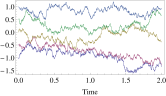
Figure 1: Single-file diffusion of Brownian point particles: individual trajectories do not cross each other.

The aim of this Letter is to present a systematic approach for calculating the cumulant generating function of the tracer position in single-file diffusion. Our analysis is based on macroscopic fluctuation theory, a recently developed framework describing dynamical fluctuations in driven diffusive systems (see Jona-Lasinio (2014); *Jona-Lasinio2010 and references therein). Specifically, we solve the governing equations of macroscopic fluctuation theory in the case of Brownian point particles with hard-core exclusion. This allows us to obtain the cumulants of tracer position and, by a Legendre transform, the large deviation function.

Macroscopic fluctuation theory also provides a simple explanation of the long memory effects found in single-file, in which initial conditions continue to affect the position of the tracer, e.g., its variance, even in the long time limit Leibovich and Barkai (2013); Lizana et al. (2014). The statistical properties of the tracer position are not the same if the initial state is fluctuating or fixed—this situation is akin to annealed versus quenched averaging in disordered systems Derrida and Gerschenfeld (2009). For general inter-particle interactions, we derive an explicit formula for the variance of the tracer position in terms of transport coefficients and obtain new results for the exclusion process.

We start by formulating the problem of tracer diffusion in terms of macroscopic fluctuation theory, or equivalently fluctuating hydrodynamics. The fluctuating density field $\rho(x,t)$ satisfies the Langevin equation Spohn (1991)

$$\partial_{t}\rho(x,t)=\partial_{x}\left[D(\rho)\partial_{x}\rho(x,t)+\sqrt{\sigma(\rho)}\eta(x,t)\right],$$ (1)

where $\eta(x,t)$ is a white noise with zero mean and with variance $\langle\eta(x,t)\eta(x^{\prime},t^{\prime})\rangle=\delta(x-x^{\prime})\delta(t-t^{\prime})$. The diffusion coefficient $D(\rho)$ and the mobility $\sigma(\rho)$ encapsulate the transport characteristics of the diffusive many-particle system, they can be expressed in terms of integrated particle current Bodineau and Derrida (2004). All the relevant microscopic details of inter-particle interactions are thus embodied, at the macroscopic scale, in these two coefficients.

The position $X_{T}$ of the tracer particle at time $T$ can be related to the fluctuating density field $\rho(x,t)$ by using the single-filing constraint which implies that the total number of particles to the right of the tracer does not change with time. Setting the initial tracer position at the origin, we obtain

$$\int_{0}^{X_{T}}\rho(x,T)dx=\int_{0}^{\infty}\left[\rho(x,T)-\rho(x,0)\right]dx.$$ (2)

This relation defines the tracer’s position $X_{T}$ as a functional of the macroscopic density field $\rho(x,t)$. Variations of $X_{T}$ smaller than the coarse-grained scale are ignored: their contributions are expected to be sub-dominant in the limit of a large time $T$. The statistics of $X_{T}$ is characterized by the cumulant generating function

$$\mu(\lambda)=\ln\left[\langle\exp(\lambda X_{T})\rangle\right],$$ (3)

where $\lambda$ is a Lagrange multiplier and the angular bracket denotes ensemble average. We shall calculate this generating function by using techniques developed by Bertini et al. Bertini et al. (2002); *Bertini2001; Jona-Lasinio (2014); *Jona-Lasinio2010, see also Derrida and Gerschenfeld (2009), to derive the large deviation function of the density profile. Starting from (1), the average in (3) can be expressed as a path integral

$$\langle e^{\lambda X_{T}}\rangle=\int\mathcal{D}\left[\rho,\hat{\rho}\right]e^{-S\left[\rho,\hat{\rho}\right]},$$ (4)

where the action, obtained via the Martin-Siggia-Rose formalism Martin et al. (1973); De Dominicis and Peliti (1978), is given by

$$S[\rho,\hat{\rho}] =-\lambda X_{T}+F[\rho(x,0)]+\int_{0}^{T}dt\int_{-\infty}^{\infty}dx$$ (5)

$$\left[\hat{\rho}\partial_{t}\rho-\tfrac{1}{2}\sigma(\rho)\left(\partial_{x}\hat{\rho}\right)^{2}+D(\rho)\,\partial_{x}\rho\,\partial_{x}\hat{\rho}\right].$$

Here $F[\rho(x,0)]=-\ln(\text{Prob}[\rho(x,0)])$ and $\hat{\rho}(x,t)$ is the conjugate response field. We consider two settings, annealed (where we average over initial states drawn from equilibrium) and quenched. In the annealed case, the large deviation function $F[\rho(x,0)]$ corresponding to the observing of the density profile $\rho(x,0)$ can be found from the fluctuation dissipation theorem which is satisfied at equilibrium. This theorem implies Spohn (1991); Derrida (2011); *Derrida2007; Krapivsky and Meerson (2012) that $f(r)$, the free energy density of the equilibrium system at density $r$, satisfies $f^{\prime\prime}(r)=2D(r)/\sigma(r)$. From this one finds Derrida (2011); *Derrida2007; Derrida and Gerschenfeld (2009)

$$F[\rho(x,0)]=\int_{-\infty}^{\infty}dx\int_{\rho}^{\rho(x,0)}dr\frac{2D(r)}{\sigma(r)}\left[\rho(x,0)-r\right],$$ (6)

where $\rho$ is the uniform average density at the initial equilibrium state. In the quenched case, the initial density is fixed, $\rho(x,0)=\rho$, and $F[\rho(x,0)]=0$.

At large times, the integral in (4) is dominated by the path minimizing the action (5). If $(q,p)$ denote the functions $(\rho,\hat{\rho})$ for the optimal action paths, variational calculus yields two coupled partial differential equations for these optimal paths

$$\partial_{t}q-\partial_{x}\left[D(q)\partial_{x}q\right] =-\partial_{x}\left[\sigma(q)\partial_{x}p\right],$$ (7a)

$$\partial_{t}p+D(q)\partial_{xx}p =-\tfrac{1}{2}\sigma^{\prime}(q)\left(\partial_{x}p\right)^{2}.$$ (7b)

The boundary conditions are also found by minimizing the action and they depend on the initial state sup . In the annealed case, the boundary conditions read

$$p(x,T) = B\theta(x-Y)\quad\text{with}\quad B=\lambda/q(Y,T),$$ (8)

$$p(x,0) = B\theta(x)+\int_{\rho}^{q(x,0)}dr\frac{2D(r)}{\sigma(r)}\,.$$ (9)

Here $\theta(x)$ is the Heaviside step function, $Y$ is the value of $X_{T}$ in Eq. (2) when the density profile $\rho(x,t)$ is taken to be the optimal profile $q(x,t)$. Note that $Y$ representing the tracer position for the optimal path (at a given value of $\lambda$) is a deterministic quantity.

In the quenched case, the initial configuration is fixed and therefore $q(x,0)=\rho$. The ‘boundary’ condition for $p(x,T)$ is the same as in (8).

In the long time limit, the cumulant generating function (3) is determined by the minimal action $S[q,p]$. Using Eqs. (7a)–(7b) we obtain

$$\mu(\lambda)=\lambda Y-F[q]-\int_{0}^{T}dt\int_{-\infty}^{\infty}dx\frac{\sigma(q)}{2}\left(\partial_{x}p\right)^{2}.$$ (10)

Thus, the problem of determining the cumulant generating function of the tracer position has been reduced to solving partial differential equations for $q(x,t)$ and $p(x,t)$ with suitable boundary conditions.

Two important properties of the single-file diffusion follow from the formal solution (10). First, since $\mu(\lambda)$ is an even function of $\lambda$, all odd cumulants of the tracer position vanish. Second, it can be shown that $\mu(\lambda)$ is proportional to $\sqrt{T}$: thus, all even cumulants scale as $\sqrt{T}$. If the tracer position $X_{T}$ is rescaled by $T^{1/4}$, all cumulants higher than the second vanish when $T\to\infty$. This leads to the well known result Arratia (1983) that the tracer position is asymptotically Gaussian.

To determine $\mu(\lambda)$ we need to solve Eqs. (7a)–(7b). This is impossible for arbitrary $\sigma(q)$ and $D(q)$, but for Brownian particles with hard-core repulsion, where $\sigma(q)=2q$ and $D(q)=1$, an exact solution can be found. In the annealed case, Eqs. (7a)–(7b) for Brownian particles become

$$\partial_{t}q-\partial_{xx}q =-\partial_{x}\left[2q\partial_{x}p\right],$$ (11a)

$$\partial_{t}p+\partial_{xx}p =-\left(\partial_{x}p\right)^{2}.$$ (11b)

The boundary conditions are (8) and (9), the latter one simplifies to

$$q(x,0)=\rho\,\exp\!\left[p(x,0)-B\theta(x)\right]$$

in the case of Brownian particles.

We treat $B$ and $Y$ as parameters to be determined self-consistently. The canonical Cole-Hopf transformation from $(q,p)$ to $Q=qe^{-p}$ and $P=e^{p}$ reduces the non-linear Eqs. (11a)–(11b) to non-coupled linear equations Elgart and Kamenev (2004); Derrida and Gerschenfeld (2009); Krapivsky et al. (2012), a diffusion equation for $Q$ and an anti-diffusion equation for $P$. Solving these equations we obtain explicit expressions for $p(x,t)$ and $q(x,t)$ sup .

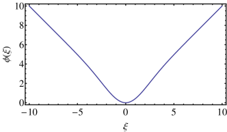
Figure 2: The large deviation function of tracer position in the case of Brownian point particles in the annealed setting with density $\rho=1$.

From this solution, the generating function $\mu(\lambda)$ is obtained in a parametric form as

$$\mu(\lambda)=\left[\lambda+\rho\frac{1-e^{B}}{1+e^{B}}\right]Y,$$ (12)

where $Y$ and $B$ are self-consistently related to $\lambda$ by

$$\lambda = \rho\left(1-e^{-B}\right)\left[1+\tfrac{1}{2}\left(e^{B}-1\right)\operatorname{erfc}(\eta)\right]$$ (13)

$$e^{2B} = 1+\frac{2\eta}{\pi^{-1/2}e^{-\eta^{2}}-\eta\,\operatorname{erfc}(\eta)}$$ (14)

where we used the shorthand notation $\eta=Y/\sqrt{4T}$.

The cumulants of the tracer position can be extracted from this parametric solution by expanding $\mu(\lambda)$ in powers of $\lambda$. The first three non-vanishing cumulants are

$$\langle X_{T}^{2}\rangle_{c} =\frac{2}{\rho\sqrt{\pi}}\sqrt{T},$$ (15a)

$$\langle X_{T}^{4}\rangle_{c} =\frac{6\left(4-\pi\right)}{\left(\rho\sqrt{\pi}\right)^{3}}\sqrt{T}$$ (15b)

$$\langle X_{T}^{6}\rangle_{c} =\frac{30\left(68-30\pi+3\pi^{2}\right)}{\left(\rho\sqrt{\pi}\right)^{5}}\sqrt{T}$$ (15c)

in the large time limit. The expression (15a) for the variance matches the well-known result Harris (1965); Spohn (1991); Leibovich and Barkai (2013). The exact solution (12)–(14), which encapsulates (15a)–(15c) and all higher cumulants, is one of our main results.

The large deviation function of the tracer position, defined, in the limit $T\to\infty$, via

$$\text{Prob}\left(\frac{X_{T}}{\sqrt{T}}=\xi\right)\sim\exp\left[-\sqrt{T}\phi(\xi)\right],$$

is the Legendre transform of $\mu(\lambda)$, given by the parametric solution (12)–(14). This large deviation function $\phi(\xi)$ can be expressed as

$$\phi(\xi)=\rho\left[\sqrt{\alpha(\xi)}-\sqrt{\alpha(-\xi)}\right]^{2},$$ (16)

with $\alpha(\xi)=\int_{\xi/2}^{\infty}dz\operatorname{erfc}(z)$. The large deviation function $\phi(\xi)$ is plotted on Fig. 2. The asymptotic formula $\phi(\xi)\simeq\rho|\xi|$ is formally valid when $|\xi|\to\infty$, but it actually provides an excellent approximation everywhere apart from small $\xi$. The expression (16) matches an exact microscopic calculation Rödenbeck et al. (1998); Hegde et al. (2014).

We carried out a similar analysis for a quenched initial condition. Here, we cite a few concrete results. The first two even cumulants read

$$\langle X_{T}^{2}\rangle_{c}= \frac{\sqrt{2}}{\rho\sqrt{\pi}}\sqrt{T},$$ (17a)

$$\langle X_{T}^{4}\rangle_{c}= \frac{2\sqrt{2}}{\rho^{3}\sqrt{\pi}}\left[\frac{9}{\pi}\arctan\left(\frac{1}{2\sqrt{2}}\right)-1\right]\sqrt{T}.$$ (17b)

These cumulants are different from the annealed case. In particular, the variance is $\sqrt{2}$ times smaller, in agreement with previous findings Lizana et al. (2010); Krapivsky and Meerson (2012); Leibovich and Barkai (2013). An asymptotic analysis yields $\phi(\xi)\simeq\rho|\xi|^{3}/12$ when $|\xi|\to\infty$. This asymptotic behavior can also be extracted from the knowledge of extreme current fluctuations Vilenkin et al. (2014).

To test our predictions, we performed Monte Carlo simulations of single-file diffusion of Brownian point particles. In most simulations, we considered $2001$ particles on an infinite line which are initially distributed on the interval $[-100,100]$. In the annealed case, the particles were distributed randomly; in the quenched case, they were uniformly spaced. The central particle is the tracer. The cumulants of the tracer position at different times, determined by averaging over $10^{8}$ samples are shown in Fig. 3. At small times (comparable to the mean collision time), the tracer diffusion is normal. At very long times, the diffusion again becomes normal since there is only a finite number of particles in our simulations. The crossover time to normal diffusion increases as $N^{2}$ with the number of particles. At intermediate times, the motion is sub-diffusive and the cumulants scale as $\sqrt{T}$. In this range the data are in excellent agreement with theoretical predictions (15a)–(15b) and (17a)–(17b).

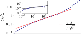
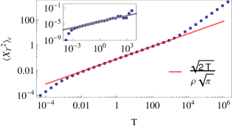
Figure 3: Simulation results for the second cumulant (main plots) and the fourth cumulant (insets). Shown are results for Brownian point particles with average density $\rho=10$ in (a) annealed and (b) quenched settings. The solid lines denote corresponding theoretical results; the variance was already computed in Leibovich and Barkai (2013).

For arbitrary $\sigma(\rho)$ and $D(\rho)$, the governing equations (7a)–(7b) are intractable, so one has to resort to numerical methods Bunin et al. (2012); Krapivsky and Meerson (2012). For small values of $\lambda$, however, a perturbative expansion of $p(x,t)$ and $q(x,t)$ with respect to $\lambda$ can be performed Krapivsky and Meerson (2012). This is feasible because for $\lambda=0$ the solution is $p(x,t)=0$ and $q(x,t)=\rho$, for both types of initial conditions. Equations (7a)–(7b) give rise to a hierarchy of diffusion equations with source terms. For example, to the linear order in $\lambda$, we have

$$\partial_{t}p_{1}+D(\rho)\partial_{xx}p_{1} = 0,$$

$$\partial_{t}q_{1}-D(\rho)\partial_{xx}q_{1} = -\sigma(\rho)\partial_{xx}p_{1},$$

where $p_{1}$ and $q_{1}$ are the first order terms in the expansions of $p$ and $q$, respectively. Solving above equations and noting that $\langle X_{T}^{2}\rangle_{c}$ is a function of the $p_{1}$ and $q_{1}$, we obtain a general formula for the variance sup

$$\langle X_{T}^{2}\rangle_{c}=\frac{\sigma(\rho)}{\rho^{2}\sqrt{\pi}}\sqrt{\frac{T}{D(\rho)}}$$ (18)

in the annealed case. In the quenched case, the variance is given by the same expression but with an additional $\sqrt{2}$ term in the denominator. We emphasize that Eq. (18) applies to general single-file systems, ranging from hard-rods Alexander and Pincus (1978) to colloidal suspensions Kollmann (2003), and also to lattice gases Arratia (1983). As an example of the latter, consider the symmetric simple exclusion process (SEP). For this lattice gas, the transport coefficients are $D(\rho)=1$ and $\sigma(\rho)=2\rho(1-\rho)$ (we measure length in the unit of lattice spacing, so $0<\rho<1$ due to the exclusion condition), so Eq. (18) yields $\langle X^{2}_{T}\rangle_{c}=2(1-\rho)\sqrt{T}/\rho\sqrt{\pi}$, in agreement with well-known results Arratia (1983). The result for colloidal suspension derived in Kollmann (2003) is recovered by inserting in (18) the fluctuation dissipation relation $\sigma(\rho)=2S(\rho)D(\rho)$, where $S(\rho)$ is the structure factor Spohn (1991).

Finding higher cumulants from the perturbative expansion leads to tedious calculations. For the SEP, we have computed the fourth cumulant

$$\langle X_{T}^{4}\rangle_{c} =\frac{2}{\sqrt{\pi}}\,\frac{1-\rho}{\rho^{3}}\,a(\rho)\sqrt{T}\,,$$

$$a(\rho) =1-\left(4-(8-3\sqrt{2})\rho\right)(1-\rho)+\frac{12}{\pi}(1-\rho)^{2}.$$

in the annealed case. For small values of $\rho$, the above results reduces to (15b). The complete calculation of the tracer’s large deviation function for the SEP remains a very challenging open problem.

To conclude, we analyzed single-file diffusion employing the macroscopic fluctuation theory. For Brownian point particles with hard-core exclusion, we calculated the full statistics of tracer’s position, viz. we derived an exact parametric representation for the cumulant generating function. We extracted explicit formulas for the first few cumulants and obtained large deviation functions. We also derived the sub-diffusive scaling of the cumulants and the closed expression (18) for the variance, valid for general single-file processes. All our results have been derived in the equilibrium situation (homogeneous initial conditions). It seems possible to extend our approach to non-equilibrium settings. Another interesting direction is to analyze a tracer in an external potential Illien et al. (2013); Barkai and Silbey (2009); Burlatsky et al. (1996, 1992) and biased diffusion Imamura and Sasamoto (2007); Majumdar and Barma (1991).

We thank S. Majumdar, S. Prolhac, T. Sasamoto and R. Voituriez for fruitful discussions, and A. Dhar for sharing results prior to publication. We are grateful to B. Meerson for crucial remarks and suggestions. We thank the Galileo Galilei Institute for Theoretical Physics for excellent working conditions and the INFN for partial support during the completion of this work.

References

- Hodgkin and Keynes (1955) A. L. Hodgkin and R. D. Keynes, Journal of physiology 128, 61 (1955).
- Kärger and Ruthven (1992) J. Kärger and D. Ruthven, Diffusion in zeolites and other microporous solids (Wiley, 1992).
- Chou and Lohse (1999) T. Chou and D. Lohse, Phys. Rev. Lett. 82, 3552 (1999).
- Meersmann et al. (2000) T. Meersmann, J. W. Logan, R. Simonutti, S. Caldarelli, A. Comotti, P. Sozzani, L. G. Kaiser, and A. Pines, J. Phys. Chem. A 104, 11665 (2000).
- Richards (1977) P. M. Richards, Phys. Rev. B 16, 1393 (1977).
- Li et al. (2009) G.-W. Li, O. G. Berg, and J. Elf, Nature Physics 5, 294 (2009).
- Kukla et al. (1996) V. Kukla, J. Kornatowski, D. Demuth, I. Girnus, H. Pfeifer, L. V. C. Rees, S. Schunk, K. K. Unger, and J. Karger, Science 272, 702 (1996).
- Wei et al. (2000) Q.-H. Wei, C. Bechinger, and P. Leiderer, Science 287, 625 (2000).
- Lutz et al. (2004) C. Lutz, M. Kollmann, and C. Bechinger, Phys. Rev. Lett. 93, 026001 (2004).
- Lin et al. (2005) B. Lin, M. Meron, B. Cui, S. A. Rice, and H. Diamant, Phys. Rev. Lett. 94, 216001 (2005).
- Das et al. (2010) A. Das, S. Jayanthi, H. S. M. V. Deepak, K. V. Ramanathan, A. Kumar, C. Dasgupta, and A. K. Sood, ACS Nano 4, 1687 (2010).
- Siems et al. (2012) U. Siems, C. Kreuter, A. Erbe, N. Schwierz, S. Sengupta, P. Leiderer, and P. Nielaba, Scientific Reports 2, 1015 (2012).
- Spohn (1991) H. Spohn, Large Scale Dynamics of Interacting Particles (Springer-Verlag, New York, 1991).
- Ferrari and Fontes (1996) P. A. Ferrari and L. R. G. Fontes, Journal of Applied Probability 33, 411 (1996).
- Alexander and Pincus (1978) S. Alexander and P. Pincus, Phys. Rev. B 18, 2011 (1978).
- Kollmann (2003) M. Kollmann, Phys. Rev. Lett. 90, 180602 (2003).
- Harris (1965) T. E. Harris, Journal of Applied Probability 2, 323 (1965).
- Levitt (1973) D. Levitt, Phys. Rev. A 8, 3050 (1973).
- Percus (1974) J. Percus, Phys. Rev. A 9, 557 (1974).
- Arratia (1983) R. Arratia, Annals of Probability 11, 362 (1983).
- Lizana and Ambjörnsson (2008) L. Lizana and T. Ambjörnsson, Phys. Rev. Lett. 100, 200601 (2008).
- Sethuraman and Varadhan (2013) S. Sethuraman and S. R. S. Varadhan, Annals of Probability 41, 1461 (2013).
- Touchette (2009) H. Touchette, Phys. Rep. 478, 1 (2009).
- Rödenbeck et al. (1998) C. Rödenbeck, J. Kärger, and K. Hahn, Phys. Rev. E 57, 4382 (1998).
- Derrida and Gerschenfeld (2009) B. Derrida and A. Gerschenfeld, J. Stat. Phys. 137, 978 (2009).
- Illien et al. (2013) P. Illien, O. Bénichou, C. Mejía-Monasterio, G. Oshanin, and R. Voituriez, Phys. Rev. Lett. 111, 038102 (2013).
- Derrida (2011) B. Derrida, J. Stat. Mech. P01030 (2011).
- Derrida (2007) B. Derrida, J. Stat. Mech. P07023 (2007).
- Jona-Lasinio (2014) G. Jona-Lasinio, J. Stat. Mech. P02004 (2014).
- Jona-Lasinio (2010) G. Jona-Lasinio, Prog. Theor. Phys. 184, 262 (2010).
- Leibovich and Barkai (2013) N. Leibovich and E. Barkai, Phys. Rev. E 88, 032107 (2013).
- Lizana et al. (2014) L. Lizana, M. A. Lomholt, and T. Ambjörnsson, Physica A 395, 148 (2014).
- Bodineau and Derrida (2004) T. Bodineau and B. Derrida, Phys. Rev. Lett. 92, 180601 (2004).
- Bertini et al. (2002) L. Bertini, A. De Sole, D. Gabrielli, G. Jona-Lasinio, and C. Landim, J. Stat. Phys. 107, 635 (2002).
- Bertini et al. (2001) L. Bertini, A. De Sole, D. Gabrielli, G. Jona-Lasinio, and C. Landim, Phys. Rev. Lett. 87, 040601 (2001).
- Martin et al. (1973) P. Martin, E. Siggia, and H. Rose, Phys. Rev. A 8, 423 (1973).
- De Dominicis and Peliti (1978) C. De Dominicis and L. Peliti, Phys. Rev. B 18, 353 (1978).
- Krapivsky and Meerson (2012) P. L. Krapivsky and B. Meerson, Phys. Rev. E 86, 031106 (2012).
- (39) See supplemental note for an outline of the derivation.
- Elgart and Kamenev (2004) V. Elgart and A. Kamenev, Phys. Rev. E 70, 041106 (2004).
- Krapivsky et al. (2012) P. L. Krapivsky, B. Meerson, and P. V. Sasorov, J. Stat. Mech. P12014 (2012).
- Hegde et al. (2014) C. Hegde, S. Sabhapandit, and A. Dhar, arXiv 1406.6191 (2014).
- Lizana et al. (2010) L. Lizana, T. Ambjörnsson, A. Taloni, E. Barkai, and M. A. Lomholt, Phys. Rev. E 81, 051118 (2010).
- Vilenkin et al. (2014) A. Vilenkin, B. Meerson, and P. V. Sasorov, J. Stat. Mech. P06007 (2014).
- Bunin et al. (2012) G. Bunin, Y. Kafri, and D. Podolsky, EPL 99, 20002 (2012).
- Barkai and Silbey (2009) E. Barkai and R. Silbey, Phys. Rev. Lett. 102, 050602 (2009).
- Burlatsky et al. (1996) S. F. Burlatsky, G. Oshanin, M. Moreau, and W. P. Reinhardt, Phys. Rev. E 54, 3165 (1996).
- Burlatsky et al. (1992) S. Burlatsky, G. Oshanin, A. Mogutov, and M. Moreau, Physics Letters A 166, 230 (1992).
- Imamura and Sasamoto (2007) T. Imamura and T. Sasamoto, J. Stat. Phys. 128, 799 (2007).
- Majumdar and Barma (1991) S. N. Majumdar and M. Barma, Phys. Rev. B 44, 5306 (1991).
See pages - of supplement.pdf