Core and filament formation in magnetized, self-gravitating isothermal layers.

Abstract

We examine the role of the gravitational instability in an isothermal, self-gravitating layer threaded by magnetic fields on the formation of filaments and dense cores. Using numerical simulation we follow the non-linear evolution of a perturbed equilibrium layer. The linear evolution of such a layer is described in the analytic work of Nagai et al. (1998). We find that filaments and dense cores form simultaneously. Depending on the initial magnetic field, the resulting filaments form either a spiderweb-like network (for weak magnetic fields) or a network of parallel filaments aligned perpendicular to the magnetic field lines (for strong magnetic fields). Although the filaments are radially collapsing, the density profile of their central region (up to the thermal scale height) can be approximated by a hydrodynamical equilibrium density structure. Thus, the magnetic field does not play a significant role in setting the density distribution of the filaments. The density distribution outside of the central region deviates from the equilibrium. The radial column density distribution is then flatter than the expected power law of $r^{-4}$ and similar to filament profiles observed with Herschel. Our results does not explain the near constant filament width of $\sim 0.1$pc. However, our model does not include turbulent motions. It is expected that accretion-driven amplification of these turbulent motions provides additional support within the filaments against gravitational collapse. Finally, we interpret the filamentary network of the massive star forming complex G14.225-0.506 in terms of the gravitational instability model and find that the properties of the complex are consistent with being formed out of an unstable layer threaded by a strong, parallel magnetic field.

1. Introduction

Molecular clouds exhibit a hierarchical density structure with stars forming in the densest regions. Often, these star-forming complexes have an elongated, filamentary shape (e.g. Schneider & Elmegreen, 1979; Johnstone & Bally, 1999; Mizuno et al., 1995; Goldsmith et al., 2008). In fact, recent observations by the Herschel Space Observatory show that parsec-scale filaments are ubiquitous in the interstellar medium (ISM) (e.g. André et al., 2010; Men’shchikov et al., 2010; Arzoumanian et al., 2011; Molinari et al., 2011). The filaments tend to extend out from dense star-forming hubs (Myers, 2009; Liu et al., 2012; Galván-Madrid et al., 2013) and, sometimes, these hub-filaments structures are part of a larger-scale pattern with parallel filaments (Busquet et al., 2013).

The filaments exhibit a nearly universal width of $\sim 0.1$ pc (measured by FWHM of the column density), independent of the central column density or length of the filament (Arzoumanian et al., 2011; Palmeirim et al., 2013). Furthermore, the radial-dependence of the column density profile is flatter than expected for an isothermal cylindrical filament in hydrostatic equilibrium (Ostriker, 1964). A number of explanations have been suggested for the observed density profiles: the filaments correspond to stagnant gas in locally colliding flows (Peretto et al., 2012), they are isothermal equilibrium cylinders in pressure-balance with the external medium (i.e. a radially-truncated cylinder in hydrostatic equilibrium; Fischera & Martin, 2012; Heitsch, 2013), or are supported by magnetic fields (Fiege & Pudritz, 2000).

Thus, the origin of the filamentary cloud structure still remains unclear and heavily debated. The clouds can be formed by compressive motions of gravitational and/or turbulent nature (Ballesteros-Paredes et al., 2007). Indeed, many numerical simulations produce filamentary structures by either isothermal driven turbulence (e.g. Padoan & Nordlund, 2002; de Avillez & Breitschwerdt, 2005; Ballesteros-Paredes & Mac Low, 2002), thermal instability in large-scale convergent flows (e.g. Vázquez-Semadeni et al., 2003; Audit & Hennebelle, 2005; Heitsch et al., 2008) or behind a shock front (e.g. Koyama & Inutsuka, 2000; van Loo et al., 2007, 2010), or by gravitational instabilities in self-gravitating sheets (e.g. Nakajima & Hanawa, 1996; Umekawa et al., 1999).

Some of the observational evidence points to a turbulent formation process for filaments and dense cores in the ISM. However, observations often show cores within clouds with linewidths that require little additional support beyond thermal pressure (e.g. Myers, 1983; Keto et al., 2004). These quiescent cores are adequately modelled by Bonnor-Ebert spheres confining the cores by self-gravity and external pressure (Bonnor, 1956; Alves et al., 2001; Tafalla et al., 2004). Such objects show that gravity plays a more prominent role than assumed in the turbulent models.

Magnetic fields are also important in the formation of the filaments. Studies comparing the orientation of the magnetic field with respect to the diffuse gas provide more insight (e.g. Li et al., 2013). Optical polarization measurements of the Taurus molecular cloud show that the magnetic field in the diffuse gas is orientated perpendicular to the axis of the B216 and B217 filaments (Goodman et al., 1992). This suggests that the filaments form as gas streams along the magnetic field lines (e.g. Ballesteros-Paredes et al., 1999). However, the long axis of the L1506 filament in Taurus and of the $\rho$ Ophiuchus clouds lies along the magnetic field (Goldsmith et al., 2008; Goodman et al., 1990).

In this paper we focus on the role of self-gravity and magnetic fields on the formation of filaments and cores within self-gravitating layers. We neglect the effect of turbulent motions (other than produced by gravitational and magnetic instabilities). Self-gravitating isothermal layers are unstable to perturbations if the exciting modes are of sufficiently long wavelength (Ledoux, 1951) and they fragment into clumps or thin filaments (Miyama et al., 1987). When the layers are threaded by magnetic fields, fragmentation still occurs. Using a linear perturbation analysis, Nagai et al. (1998) show that, for a layer with a thickness larger than the pressure scale height, the magnetic field suppresses the growth of perturbations perpendicular to the field. Perturbations along the field are unaffected so that parallel filaments form within the slab. On the other hand, for a layer with a thickness smaller than the scale height, filaments form with their axis orientated along the magnetic field. The separation of the filaments is given by the wavelength of the fastest growing mode. The filaments then condense into clumps and dense cores as long as the filaments are in a quasi-static equilibrium (Inutsuka & Miyama, 1992).

We extend the study of Nagai et al. (1998) into the non-linear regime and discuss the resulting structures. In Sect. 2 we describe the initial conditions of the self-gravitating layer and the numerical model used. Then, we discuss the fragmentation of the layer in absence (Sect. 3) and presence of a parallel or perpendicular magnetic field (Sect. 4 and 5). In Sect. 6 we interpret the structure of the molecular cloud G14.225-0.506 in terms of the discussed gravitational instability model. Finally, we conclude and discuss our results in Sect. 7.

2. Model set-up

2.1. Initial conditions

For our initial conditions we assume a self-gravitating isothermal layer that extends to infinity along the $x,y$-plane. The layer is initially in hydrostatic equilibrium, so that the density distribution along the $z$-axis is given by (Spitzer, 1942)

$$\rho(z)=\rho_{0}\ {\rm sech}^{2}(z/H),$$ (1)

with $H=a/\sqrt{2\pi G\rho_{0}}$ the pressure scale height, $a$ the isothermal sound speed, $G$ the gravitational constant and $\rho_{0}$ the unperturbed density at the midplane (i.e. at $z=0$). The layer is truncated at $\pm z_{B}$ and confined by a constant external thermal gas pressure $p_{\rm g,ext}=a^{2}\rho(z_{B})$. In this paper we will not study the effect of the external pressure on fragmentation. Therefore, we only consider a layer bounded by a low external pressure, i.e. $p_{\rm g,ext}\ll p_{\rm g,0}$. We adopt $z_{B}=2H$, so that $p_{\rm ext}=0.071p_{\rm g,0}$.

Outside the layer, not only the pressure, but also the density, $\rho_{\rm ext}$, is kept constant at a small fraction of the density at the boundary (see later for exact value). This means that the external temperature differs from the internal temperature. We, therefore, modify the isothermal equation of state to be

$$p_{\rm g}=\rho\left((1-\alpha)\frac{p_{\rm ext}}{\rho_{\rm ext}}+\alpha a^{2}\right).$$ (2)

This reflects the difference in external and internal temperature with $\alpha$ a scalar that is 1 inside the layer and 0 outside.

The layer and the external medium are threaded by a uniform magnetic field. For parallel models the magnetic field is along the $x$-axis, while, for perpendicular models, it is along the $z$-axis. The field strength is given by $\beta=p_{m}/p_{g}$ at the midplane with $p_{m}=B^{2}/2$ the magnetic pressure. For our models we use $\beta=\infty{\rm\ (i.e.\ no\ magnetic\ field)},10,1{\rm\ and}\ 0.1$. For simplicity, our simulations are performed dimensionless. We adopt $\rho_{0}=2\pi$, $G=1$ and $a=1$ so that $H=1/2\pi$ and the dynamical time $t_{\rm dyn}=1/\pi$. The free-fall time associated with gas at the midplane is $\sim 1/5$. For a layer with a central density of $1000~{}{\rm cm^{-3}}$ (and thus a surface density of $\approx 10^{21}~{}{\rm cm^{-2}}$) and a temperature of 10 K, these values correspond to $H=0.159$ pc, $B=27~{}{\rm\mu G}$ (for $\beta=1.0$) and $t_{\rm dyn}=1.57$ Myr. In the rest of the paper we will evaluate the dimensionless results in terms of this layer.

This set-up is similar to the one used in the linear analysis of Nagai et al. (1998) allowing a comparison between analytically and numerically derived growth rates of the gravitational instability. To study the gravitational instability of a pressure-confined self-gravitating layer, we perturb the equilibrium state. We do this in two different ways, i.e. we superimpose the density either with a sinusoidal density perturbation of a given wavelength or with randomly generated noise. The former is used to determine the growth rates to compare with analytic values, while the latter shows how different wave modes interact with each other. From the linear analysis Nagai et al. (1998) suggest that first the filaments form and only then the dense cores.

2.2. Numerical code and domain

To solve the ideal magnetohydrodynamics (MHD) equations we use the Adaptive Mesh Refinement (AMR) MHD code MG (Van Loo et al., 2006; Falle et al., 2012). The basic algorithm is a second-order Godunov scheme with a linear Riemann solver (Falle, 1991). To ensure that the solenoidal constraint is met, a divergence cleaning algorithm is implemented in the numerical scheme (Dedner et al., 2002). A hierarchy of grids levels is used with a mesh spacing on grid level $n$ of $\Delta x/2^{n}$ with $\Delta x$ the cell size at the coarsest level. While the two coarsest levels cover the entire domain, finer levels generally do not. Refinement is on a cell-by-cell basis and is controlled by error estimates based on the difference between solutions on different grid levels. Self-gravity is computed using a full approximation multigrid to solve the Poisson equation.

The numerical domain is given by $-2~{}<~{}z~{}<~{}2$ and $-L/2~{}<~{}x,y~{}<L/2$ where $L$ is either $\lambda_{crit}/2,\lambda_{\rm crit},\lambda_{\rm max}\ {\rm or}\ 4\lambda_{\rm max}$. Here, $\lambda_{\rm crit}=2\pi H$ is the critical wavelength below which the gravitational instability is suppressed and $\lambda_{\rm max}=4\pi H$ the wavelength for which the growth rate is maximal (see Nagai et al., 1998). For our adopted values, $\lambda_{\rm crit}\approx 1$ and $\lambda_{\rm max}\approx 2$. As the layer is assumed to be infinite, we set the boundary condition on both the $x$ and $y$-axis to periodic. For the $z$-axis we use free-flow boundary conditions.

The resolution of the simulation is set by the vertical extent of the slab. It is necessary to properly resolve the pressure scale height $H$ in order to find a proper balance between pressure gradients and self-gravity. We resolve the scale height by at least 5 cells. Therefore, we use an AMR mesh with the coarse level having 4 grid cells along the axis with the shortest length (along the $x,y$-axis for the runs up to $L=\lambda_{\rm max}$ and along the $z$-axis for $L=4\lambda_{\rm max}$) and 128 cells along the $z$-axis for the finest grid level. This means that the number of additional grid levels varies with different models, i.e. from 2 extra grid levels for $L=\lambda_{\rm crit}/2$ up to 5 grid levels for $L=4\lambda_{\rm max}$. This resolution is more than sufficient to resolve the Jeans’ length as suggested by Truelove et al. (1997) to avoid artificial fragmentation. In fact, artificial fragmentation is only expected above $\rho>\pi a^{2}/16G\Delta x^{2}\approx 200$.

As we are interested in the gravitational instability in the equilibrium layer, we need to ensure that the external medium does not affect the gravitational instability in the layer in any way. By assuming a constant pressure in the external medium, the external medium needs to be a vacuum. (The gravitational force is zero if there is no pressure force.) However, in a grid code, we cannot set the density to zero. For a non-zero external density, the self-gravity of the layer drags the external medium towards it. Then the external medium affects the hydrostatic layer because gas is accreted onto the layer and because the ram pressure contributes to the total external pressure. We find that the external density needs to be at most $10^{-4}\ \rho(z_{\rm B})$ not to affect the equilibrium layer. As the external pressure is $\rho(z_{\rm B})a^{2}$, this means that the external sound speed is $10^{2}$ times larger than in the layer. This significantly limits the stable numerical time step derived from the Courant condition $\approx\Delta x/a$. Because of this constraint, we use a different approach, i.e. we artificially switch off the self-gravity in the external medium. This is easily done as the different media have a different value of the scalar $\alpha$. This intervention allows us to set the external medium density to $0.1\ \rho(z_{\rm B})$ without affecting the equilibrium layer and gives us a speed up of more than a factor of ten in computational time.

3. No magnetic field

In order to determine the effect of the magnetic field on the density distribution and geometry of the filaments, we first study the onset and evolution of the gravitational instability in the absence of a magnetic field. We start by confirming the theoretically derived growth rates and continue by examining the interaction of different wave modes.

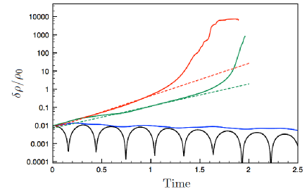
Figure 1.— The temporal evolution of the normalized density perturbation amplitude for a wave mode with a wavelength $\lambda_{\rm crit}/2$ (black), $\lambda_{\rm crit}$ (blue), $\lambda_{\rm max}$ (red) and $4\lambda_{\rm max}$ (green). The dashed lines show the linear evolution using the theoretically derived growth rates. For a layer with a central density of $1000~{}{\rm cm^{-3}}$, i.e. our default layer, a unit of time is $\sim 4.9$Myr.

Growth rates

Figure 1 shows the evolution of the maximum density perturbation amplitude for modes with a wavelength of $\lambda_{\rm crit}/2$, $\lambda_{\rm crit}$, $\lambda_{\rm max}$ and $4\lambda_{\rm max}$. The initial amplitude of the perturbation is 1% of the local density. For a perturbation with a wavelength below $\lambda_{\rm crit}$, the amplitude of the perturbation gradually decreases. The wave mode is damped and the self-gravitating layer is stable under such a perturbation. This remains so until the wavelength of the perturbing mode reaches $\lambda_{\rm crit}$. This critical wavelength (hence $\lambda_{\rm crit}$) has a zero growth rate and the amplitude of the critical wave mode remains roughly constant for multiple dynamical time scales. It also marks the transition to a layer that is unstable to perturbations with $\lambda>\lambda_{\rm crit}$. Our simulations reproduce the theoretically derived linear growth rates of Nagai et al. (1998) for these longer wavelength perturbation very well. During the linear growth phase, the amplitude of the perturbation grows as $\sim\exp(\omega t)$. For the fastest growing wave mode with wavelength $\lambda_{\rm max}$, we find $\omega\approx 4.12$, which is close to the analytically derived value of $\omega\approx 4.49$ (Elmegreen & Elmegreen, 1978). For $4\lambda_{\rm max}$, $\omega\approx 2.81$ and is similar to the value inferred from Fig. 1 of Nagai et al. (1998). Note that the linear growth phase ends when $\delta\rho\approx\rho_{0}$ and the growth becomes non-linear. This non-linear growth phase lasts until nearly all the gas of the layer is concentrated in a single dense filament which is starting to fragment into cores. We do not have sufficient resolution to follow this fragmentation and, at this time, we end the simulation.

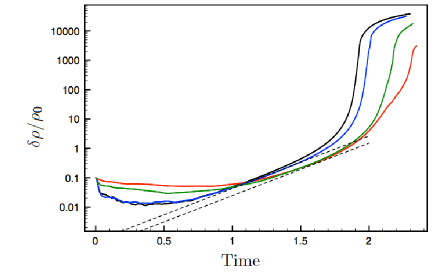
Figure 2.— The temporal evolution of the normalized density perturbation (solid line) when random density perturbations are imposed on the equilibrium slab for a hydrodynamical (black), $\beta=10$ (blue), 1 (green) and 0.1 (red) model. The dashed lines shows the linear growth of a wave mode with a wavelength $\lambda_{\rm max}$. For our default layer, unit of time is $\sim 4.9$Myr.

Filament and core formation

We have confirmed the growth rates for different wave modes, but we need to understand how the different wave modes interact with each other. Therefore, we superimpose the equilibrium density with random noise. The maximal amplitude of the density noise is 10% of the local density. We allow wave modes with a wavelength up to $4\lambda_{\rm max}$ to develop within the layer, i.e. the numerical domain is $-2\lambda_{\rm max}<x,y<2\lambda_{\rm max}$. Figure 2 shows the maximum amplitude of the density perturbations. Initially, as we impose random noise at the grid level, the wave modes have a wavelength below $\lambda_{\rm crit}$. These modes are stable and the amplitude thus decreases. However, wave modes with longer wavelengths for which the layer is unstable are excited and gradually grow. The fastest growing unstable wave mode, i.e. the mode with a wavelength $\lambda_{\rm max}$, becomes dominant. This can be clearly seen in Fig. 2 as the evolution of the maximum perturbation amplitude can be described by the linear growth phase of that wave mode.

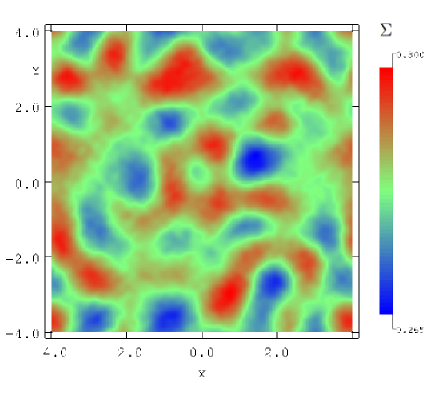
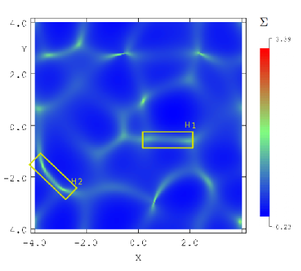
Figure 3.— The logarithmic surface density along the $z$-axis for a layer without magnetic fields at $t=1$ (top) and at $t=2$ (bottom). The boxes show filaments selected for further analysis. In terms of our default layer, the area shown is 8$\times$8 pc² and the unit of surface density is 5$\times$10${}^{20}~{}{\rm cm^{-2}}$.

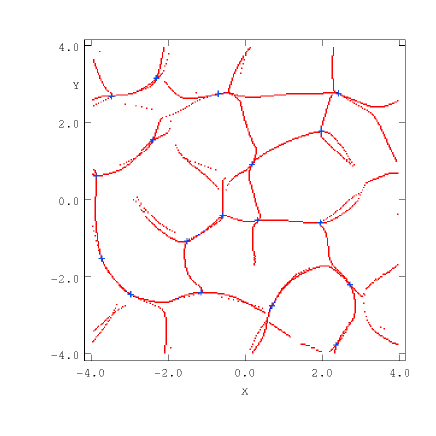
Figure 4.— Ridge identification for the column density of the bottom panel in Fig. 3. The local maxima are indicated by blue crosses.

Figure 3 shows the resulting surface density integrated along the $z$-axis at two different times, i.e. at the beginning of the linear growth phase at $t=1$ and near the end of the non-linear growth phase at $t=2$. A network of interconnecting filaments with embedded cores has formed. Note that regions of high column density are already present early on in the linear phase. In fact, there is a one-to-one correlation. To better understand the interplay between the different filaments and the positions of the cores, we use a ridge finding algorithm to expose the skeleton of the network and to locate column density maxima (e.g. Lindeberg, 1998). The ridges and local maxima for the bottom panel of Fig. 3 are shown in Fig. 4. Note that filaments have a separation of about $\lambda_{\rm max}$ indicating that the filaments are indeed formed by the most unstable wavelength (as already inferred from the growth rates). Although, in the absence of magnetic fields, the most unstable wave mode has the same growth rate in all directions, filaments predominantly form along the $x$ and $y$ axes. This is most likely because the flow equations are evolved along the Cartesian coordinate axes in the numerical code and thus excite the wave modes along these directions. Another interesting feature is that the local maxima, i.e. dense cores, lie at the intersections of the filaments. This is reminiscent of the hub-filament structures discussed by Myers (2009) and the network of filaments seen in the Herschel observations of the Rosette molecular cloud and Pipe nebula (Schneider et al., 2012; Peretto et al., 2012). Such a network is also present in cloud formation simulations which include turbulence (e.g. Vázquez-Semadeni et al., 2003), but is generated due to dynamical (other than gravity) and thermal instabilities. Other random noise initializations produce a similar network of filaments with a separation of about $\lambda_{\rm max}$ and dense cores at the intersections of filaments.

Radial profile of filaments

Several authors (e.g. Arzoumanian et al., 2011; Palmeirim et al., 2013; Kirk et al., 2013) characterise the filaments by mapping the observed column densities with Plummer-like profiles. They assume that the underlying density profile of the cylindrical filament is given by

$$\rho(r)=\frac{\rho_{0}}{\left[1+\left(r/R_{0}\right)^{2}\right]^{\frac{p}{2}}},$$ (3)

where $r$ is the cylindrical radius, $R_{0}$ the characteristic radius of the flat inner region and $p$ the power-law index of the profile at large radii. For $p=4$, this profile describes an isothermal cylinder in hydrostatic equilibrium with $R_{0}=\sqrt{2a^{2}/\pi G\rho_{0}}$ the scale height (Ostriker, 1964). The resulting column density profile (assuming that the filament lies within the plane perpendicular to the integration) is also a Plummer-like profile given by

$$\Sigma(l)=\frac{B_{p}\rho_{0}R_{0}}{\left[1+\left(l/R_{0}\right)^{2}\right]^{\frac{p-1}{2}}},$$ (4)

where $B_{p}$ is the Euler beta function with input values $1/2$ and $(p-1)/2$ and $l$ the projected radius.

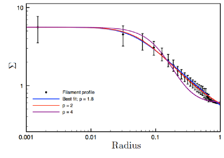
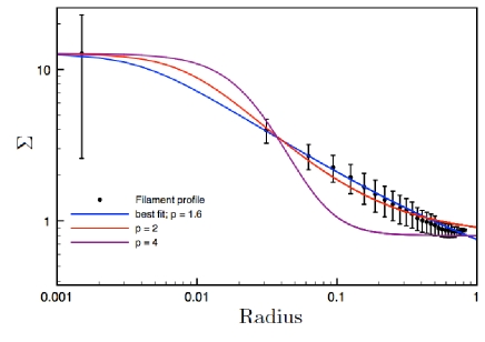
Figure 5.— Radial column density profile for two selected regions in Fig. 3: Region H1 is on the top panel, while Region H2 is on the bottom one. We display the central column density at a radius of 0.0015 and not at a radius of 0.0. The solid circles show the column densities at a given radius from the filament axis averaged over the entire filament while the error bars are the dispersion on the mean. The blue line is the best fit Plummer-profile with a background column density, while the red and purple lines show the Plummer-like profile for $p=2$ and $p=4$, respectively. For our default layer, the unit of length is 1 pc and the unit of surface density is 5$\times 10^{20}~{}{\rm cm^{-2}}$.

We extract several filaments from the column density map at $t=2$. For each filament, we derive the radial distributions perpendicular to the axis at each cell along the filament axis. By combining all the distribution along a filament axis we obtain the average radial distribution of the filament. Note that, for curved filaments, radial profiles will cross each other, but this will not strongly influence the average radial distribution as long as the curvature is small. We then fit the average distribution with the theoretical profiles of Eq. 4. We add a constant background column density because the filaments are embedded in a layer.

Figure 5 shows the profiles and fits for two filaments. The best fit for Region H1 is given by $p=1.8$, $R_{0}=0.045$ and $\rho_{0}=26.9$, while $p=2$ still produces a good fit. However, an equilibrium model with $p=4$ cannot reproduce the filament profile at all. A similar result is found for Region H2 where the best fit is $p=1.6$, $R_{0}=0.004$ and $\rho_{0}=683$. These results agree well with observationally derived values of $1.5<p<2.5$ by Arzoumanian et al. (2011) and others. The value of $R_{0}$, however, varies significantly between the different filaments. For Region H1 the inner flat region is about an order of magnitude larger than in Region H2.

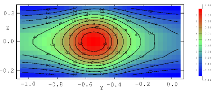
Figure 6.— Density cross-section of the filament in Region H1 of Fig. 3 at $x=1.25$ with contour lines. For the default layer, the units of density and length are 159.2 ${\rm cm^{-3}}$ and 1 pc, respectively.

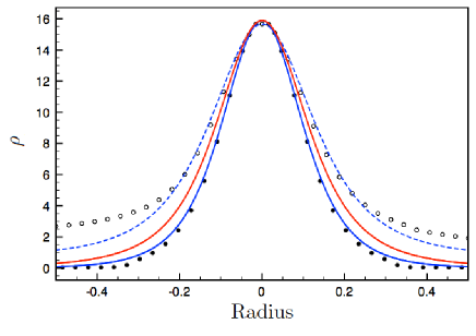
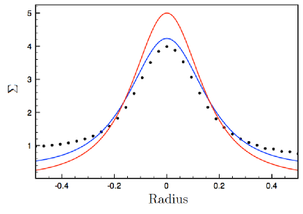
Figure 7.— Top: Density slices along the coordinate axes for Fig. 6. The open circles are along the $y$-axis and the solid ones along the $z$-axis. The blue lines (solid along $z$-axis and dashed along $y$-axis) are the best fit model for a Schmidt-Burgk profile, i.e. $A=0.6$ and $\rho_{c}=3.976$, while the red line is the expected profile for an equilibrium cylinder with $\rho_{0}=15.9$. For our default layer, the unit of density is 159.2 ${\rm cm^{-3}}$. Bottom: Column density profile of the same figure. The dots are the simulation values, while the blue, resp. red, solid lines are the expected column density for the Schmidt-Burgk profile, resp. the Ostriker profile. The unit of surface density corresponds to 5$\times 10^{20}~{}{\rm cm^{-2}}$, while the unit of length is 1 pc.

The average radial column density profiles suggest that the filaments are far from equilibrium. Numerical simulations provide the opportunity to confirm this claim directly from the density distribution. We examine different slices across the filament in Region H1. Figure 6 shows one of these cross sections. Although the center of the filament is nearly axisymmetric, the outer layers are flattened along the slab. An equilibrium profile (Ostriker, 1964) provides a good fit to the central region of the filament, but cannot explain the asymmetry along the different axes (see Fig. 7). This, however, does not imply that the structure is far from equilibrium. Actually, the cross section is reminiscent of a modulated self-gravitating layer in equilibrium (Curry, 2000; Myers, 2009). The density distribution of such a modulated layer is given by (Schmid-Burgk, 1967)

$$\rho=\rho_{c}\frac{1-A^{2}}{\left(cosh(z/L)-A\ cos(x/L)\right)^{2}},$$ (5)

where $\rho_{c}$ is the midplane density of the unmodulated layer, $A$ the modulation factor between 0 and 1 and $L=a/\sqrt{2\pi G\rho_{c}}$ the scale height. For $A=0$ we find the Spitzer solution for a infinite layer, i.e. Eq. 1, while, for $A\rightarrow 1$, it converges to the Ostriker (1964) solution for an infinite cylinder. By applying a Schmid-Burgk profile to density slices through the center of the cross section shown in Fig. 6 and along the $y$ and $z$ coordinate axes, we find that the density profile of the filament is best reproduced with $A=0.6$ and $\rho_{c}=3.976$ (see Fig. 7). The fit is good for radii up to the scale height $L=0.2$ above which the density along the midplane is higher. Other slices of the filament can also be described by a Schmid-Burgk profile albeit with somewhat different values of $A$ and $\rho_{c}$ (i.e. $0.55<A<0.65$ and $4<\rho_{c}<7.5$). This variation implies a density variation along the filament axis and reflects that cores are embedded within a filament.

By integrating Eq. 5 along the $z$-axis and using the derived parameters $A$ and $\rho_{c}$, we find that the Schmid-Burgk profile reproduces not only the density profile, but also the column density profile (see Fig. 7). Again the fit is best for radii below the scale height, but it exhibits a flatter radial distribution than the (Ostriker, 1964) profile. This partly explains the flatter than the Ostriker equilibrium radial profile observed in the mean column density distribution (Fig. 5). Some of the flattening is due to averaging profiles with marginally different parameters.

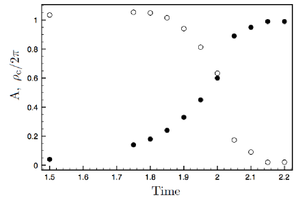
Figure 8.— Evolution of the filament profile as function of time. The solid circles are the values for $A$, while the open ones are the values of $\rho_{c}$ normalized to the initial value. In terms of our default layer, a unit of time is 4.9Myr.

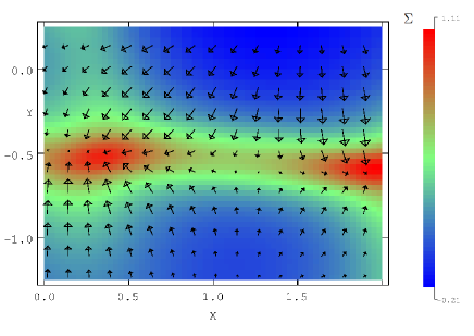
Figure 9.— Logarithmic column density for Region H1 of Fig. 3. The vectors represent the mass-weighted velocities in the plane. Their size is an indication of their magnitude with the maximal velocity shown $1.6$ times the sound speed. Remember that the unit of column density is 5$\times 10^{20}~{}{\rm cm^{-2}}$ and that the sound speed is $\approx 0.2~{}{\rm km\ s^{-1}}$ in our default layer.

Evolution of the filaments

Although the density profile shows a filament close to equilibrium, it is in fact dynamically evolving. The filament profile changes with time, but can, at all instances, be described by a Schmid-Burgk profile (see Fig. 8). Initially, the filament is only a small perturbation on top of the equilibrium layer (i.e. $A\approx 0$), while it evolves towards an equilibrium cylinder at the end of the non-linear phase (i.e. $A\approx 1$). The evolution of a filament thus occurs through a sequence of quasi-equilibrium distributions. Note that $\rho_{c}$ does not remain constant during the evolution. This suggests that gas does not accumulate in this filament segment. Figure 9 indeed shows that, while gas flows towards the filaments, it is then diverted towards denser regions (cores) along the filament axis.

The evolution of the filaments is set by the mass that the gravitational instability sweeps up. The expected line mass is essentially determined by the wavelength of the fastest growing wavelength and given by $m_{\rm line}\approx\Sigma_{0}\lambda_{\rm max}$ with $\Sigma_{0}\approx 2\rho_{0}H$ the column density of the equilibrium layer. This value needs to be compared with the critical value for the line-mass of a stable cylinder, i.e. $m_{\rm crit}=2a^{2}/G$ (Ostriker, 1964). For our model parameters, $m_{\rm line}\approx 1.9m_{\rm crit}$. We can also derive line-masses for different cross-sections in filaments. For example, we find $m_{\rm line}\approx 2.6$ for Fig. 7). While this is less than the predicted value, it still exceed the critical value of $m_{\rm crit}=2$. It is interesting to note that half of the line-mass lies within the central region bound by the scale height. Thus, the filament is collapsing radially while maintaining a quasi-equilibrium for radii up to the scale height.

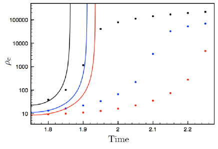
Figure 10.— The evolution of the central density of three selected cores in the hydrodynamical simulation (full circles). Each core is represented by a different color (black, blue or red). The solid lines show the evolution of the central density for homologous collapse of a uniform sphere for each core (in the same color). In terms of the default layer, a unit of time equals 4.9Myr and a unit of density 159.2 cm^-3.

Evolution of the dense cores

As mentioned earlier, the dense cores arise at the junctions of the filaments. The cores are elongated along the axis of the most dense filament. As they evolve, the cores become more centrally condensed (see Fig. 10).

The cores collapse at a rate that is slower than expected for pressureless gravitational, i.e. homologous, collapse of a uniform sphere (the free-fall time is between 0.1 and 0.2 for all the cores). There are two main reasons. Firstly, the cores are embedded in and are formed out of cylindrical filaments. Mass accretion towards the cores is thus not isotropic but highly directional. Toalá et al. (2012) and Pon et al. (2012) show that the collapse time scales of non-spherical structures are longer than the corresponding spherical free-fall time scale. In the case of a cylindrical cloud, the time-scale depends strongly on the aspect ratio of the cloud. Note that the above authors only consider the collapse of constant mass structures. The mass of the filaments does change in our simulation. However, as the line mass of the filament is set by the fastest-growing wavelength, the mass of the filaments does not change significantly once the evolution is in the non-linear regime.

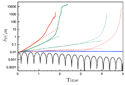
Figure 11.— The temporal evolution of the normalized density perturbation for perturbations with a wavelength $\lambda_{\rm crit}/2$ (black), $\lambda_{\rm crit}$ (blue), $\lambda_{\rm max}$ (red) and $4\lambda_{\rm max}$ (green). The thin solid lines are for perturbations along the $y$-axis. The dashed lines show the linear evolution using the theoretically derived growth rates. As before, the unit of time corresponds to 4.9Myr for our default layer.

Secondly, the assumption of pressureless collapse is not valid. The results for the filaments show that the inner region can be adequately described by an equilibrium profile in which self-gravity is nearly balanced by thermal pressure. Inutsuka & Miyama (1992) show that, in the case of equilibrium cylinders, this significantly reduces the collapse rate. As cores form out of filaments, it is likely that the thermal pressure plays a similar role in cores. However, we cannot easily test this hypothesis as there is no analytic solution for an equilibrium core within a cylindrical filament (and certainly not for a core in a Schmid-Burgk like filament). Furthermore, the accretion of gas is not along one filament, but multiple ones complicating the expected structure even more.

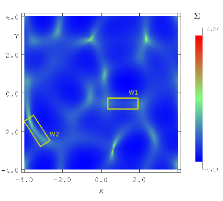
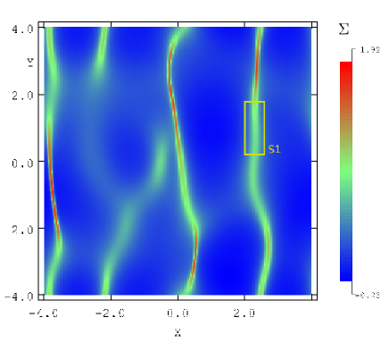
Figure 12.— Surface density along $z$-axis for the $\beta=10$ model at $t=2$ (top) and the $\beta=0.1$, model at $t=2.25$ (bottom). In terms of the default layer, the area shown is 8$\times$8 pc² and the unit of surface density is 5$\times 10^{20}~{}{\rm cm^{-2}}$.

4. Parallel magnetic field

Growth rates

The analysis of Nagai et al. (1998) shows that the gravitational instability in an equilibrium layer is modified by magnetic fields as they stabilize instabilities propagating perpendicular to the field (when the external pressure is small). Instabilities along the magnetic field are not affected. The effect of the magnetic field is expressed as a function of a dimensionless parameter $\alpha^{\prime}$ which for our model parameters is given by $\alpha^{\prime}=2.15/\beta$. Thus, our models examine a range of $\alpha^{\prime}$ between 0.215 and 21.5. For values as low as $\alpha^{\prime}=1.25$ (i.e. $\beta=2$) the perpendicular perturbations are already strongly suppressed (see e.g. Fig. 4 of Nagai et al. (1998)).

Similar to the hydrodynamical simulations we first examine whether our numerical model reproduces the expected linear growth rates. We only test this for $\beta=0.10$ (i.e. $\alpha^{\prime}=21.5$). For perturbations along the magnetic field (i.e. along the $x$-axis), we find, as expected, linear growth rates that are marginally smaller than in the hydrodynamical model (see Fig. 11). The critical wavelength and the maximal wavelength are also the same as before. For perpendicular perturbations along the $y$-axis, the growth rates are significantly reduced. For $\lambda_{\rm max}$ we find $\omega\approx 0.25$ or about 20 times lower than for an identical perturbation along the $x$-axis, while we have $\omega\approx 0.85$ when $4\lambda_{\rm max}$. Note that the growth rate for $4\lambda_{\rm max}$ is larger than for $\lambda_{\rm max}$ as $\lambda_{\rm max}$ is here the value for the fastest growing wave mode along the $x$-axis and not the $y$-axis. The critical and maximal wavelength along the $y$-axis are shifted towards longer wavelengths, i.e. $\lambda_{\rm y,max}\approx 2.5\lambda_{\rm max}$ and $\lambda_{\rm y,crit}\approx 1.8\lambda_{\rm crit}$. The shown models for perturbations perpendicular to the magnetic field then represent models close to the critical and maximal wavelength.

The simulations confirm the behavior derived from the linear analysis and show that the magnetic field introduces a preferred direction for the growth of perturbations, even for high values of $\beta\ (>1)$.

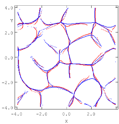
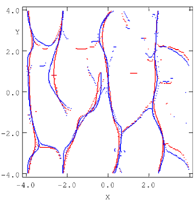
Figure 13.— Ridges of column density for the weak magnetic field (red) and hydrodynamical (blue) model at $t=2$ (top) and for $\beta=0.1$ (red) and $\beta=1$ (blue) at $t=2.25$ (bottom).

Filament formation

We superimpose the equilibrium layer with the same random noise perturbations as the hydrodynamical model. Figure 2 shows the normalized maximum perturbation amplitude for $\beta=10,\ 1,\ {\rm and}\ 0.1$ (as well as for $\beta=\infty$, i.e. the hydrodynamical model). The linear phase of the instability shows, for all of the magnetic models, the typical growth rate of a mode with a wavelength of $\lambda_{\rm max}$. That this specific wave mode is dominant also becomes apparent from the column density structure (see Fig. 12). As the perpendicular perturbations are significantly damped for the $\beta=0.1$ model (see above), only the modes parallel to the magnetic field become unstable. Four parallel filaments are then produced with an separation of about $\lambda_{\rm max}$. Note that the $\beta=0.1$ model is shown at $t=2.25$ and not $t=2$ as it reaches similar densities at later times than in the $\beta=10$ model.

Although the layer is threaded by a magnetic field, the column density structure of the $\beta=10$ model shows filaments both parallel and perpendicular to the magnetic field direction. In fact, the column density structure is very similar to the structure seen in the hydrodynamical model. Actually, the positions of the filament ridges are identical in both models (see Fig. 13). The ridge positions for the stronger magnetic field models (i.e. $\beta=1$ and 0.1) are also interchangeable. Remember that the density initialization is identical for all models and the subsequent evolution is then determined by the growth of the unstable modes. This means we can identify two different regimes, i.e. a quasi-hydrodynamical regime and a strong magnetic field one. The separation between the two states lies somewhere between $\beta=2$ and 10.

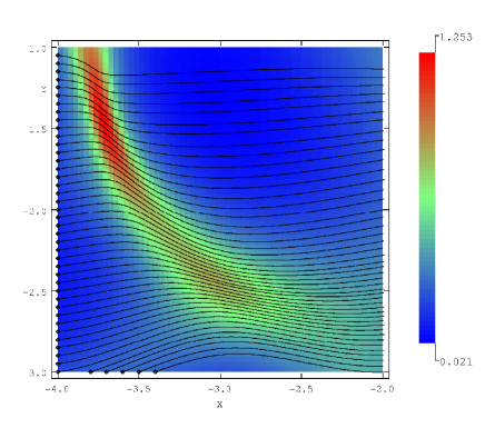
Figure 14.— The column density of Region W1 with the vectors showing the mass-weighted magnetic field. Their length indicates the magnetic field magnitude with the maximum about 3 times the initial magnitude. In terms of the default layer, the unit of column density is 5$\times 10^{20}~{}{\rm cm^{-2}}$ and the maximum magnetic field strength displayed is 6$\mu$G.

Not only the density structure, but also the magnetic field structure is distinctively different in the two regimes. In the strong magnetic regime, the magnetic field is dynamically important and suppresses perturbations perpendicular to its orientation. Then gas flows are predominantly along the magnetic field lines resulting in filaments perpendicular to the magnetic field. Contrary, in the weak magnetic regime, the magnetic field is dynamically passive and is dragged with the gas. Consequently, the density structures lie not only perpendicular to the field lines, but also parallel and oblique.

For the oblique filaments an interesting phenomenon occurs: while the magnetic field is oblique to the filament axis in the outer regions of the filament, it is orientated along the filament axis within its central region (see Fig. 14). The filaments are bound by fast-mode shocks in which the magnetic field increases perpendicular to the shock normal. The formation of such filaments is described in Nakajima & Hanawa (1996) who show that such filaments are in quasi-static equilibrium in their inner parts.

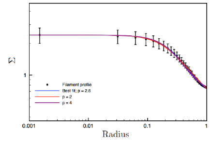
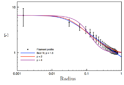
Figure 15.— Radial column density profiles for Region W1 (top) and Region W2 (bottom) averaged over the entire filament. The error bars show the dispersion on the mean value at a given radius. The solid lines show the best fit (blue), a $p=2$ (red) and $p=4$ (purple) Plummer profile. For the default layer, the units of column density and length are 5$\times 10^{20}~{}{\rm cm^{-2}}$ and 1 pc, respectively.

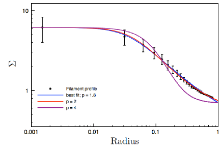
Figure 16.— Average radial column density profile for Region S1 with the dispersion on the mean given by the error bars. The solid lines show the best fit (blue), a $p=2$ (red) and $p=4$ (purple) Plummer profile. For the default layer, the units of column density and length are 5$\times 10^{20}~{}{\rm cm^{-2}}$ and 1 pc, respectively.

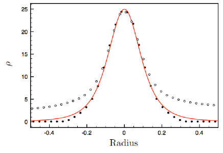
Figure 17.— Density slice at $y=1$ for Region S1. The solid circles show the density along the $z$-axis and the open circles along the $x$-axis. The solid line is the profile for an Ostriker cylinder with $\rho_{c}=24.9$. In terms of the default layer, the length unit is 1 pc and the density unit 159.2 cm^-3.

Radial filament profile

The average radial column density profile for the filaments in the magnetized layers is similar to the profiles extracted for the hydrodynamical model (see Figs. 15 and 16). The distribution is best fitted by Plummer profiles (Eq. 3) with power-law indices $p\leq 2$ and cannot be fitted by an equilibrium profile with $p=4$. An exception is Region W1 which can be fitted reasonably well by a large range of $p$-values, including $p=4$. The ratio of the central-to-external column density for Region W1 is small. The distribution then does not sample the power-law tail of the Plummer profile properly as the distribution is dominated by the flat inner region and the background column density. This results in a broad range of possible power-law indices for the Plummer profile.

Again, density slices through the filaments show that the density distribution of the central region can be approximated by an equilibrium Schmid-Burgk profile. For example, the density distribution for a slice at $x=1.25$ in Region W1 is best fitted with $A=0.13$ and $\rho_{c}=4.825$. A slice through $y=1$ of Region S1 is best fitted by an Ostriker cylinder (or a Schmid-Burgk profile with $A=1$) with $\rho_{c}=24.9$ (see Fig. 17). The selection of these filaments represents different stages during the formation process, i.e. the filament of Region W1 is starting to form, while Region S1 shows the end of the formation process. Although the interpretation from the density profiles seems inconsistent with the one inferred from the average column density distribution, it is not. For filaments exceeding the critical line-mass, the density distribution is described by an equilibrium profile only for radii below the scale height. The excess mass is at radii above the scale height resulting in a radial profile flatter than $r^{-4}$. As the Plummer profile only measures the radial dependence at radii above the scale height, such a description misses the equilibrium distribution in the center of the filament.

A more important result is that the filaments can be approximated by a hydrodynamical equilibrium without adjusting the sound speed (to take into account additional support provided by magnetic support). This suggests that the magnetic field is not important in setting the density distribution inside of the filaments. In filaments perpendicular to the magnetic field, gas flows along the field lines. Then magnetic pressure gradients are not generated and are thus much smaller than pressure (or density) gradients. In the quasi-hydrodynamical regime, filaments also form parallel to the magnetic fields. Because of magnetic flux conservation, a scaling of the magnetic field with density is established, i.e. $B\propto\rho$. The magnetic pressure, then, has a similar slope as the thermal pressure. However, as $\beta>1$, the magnetic pressure gradient is still much smaller than the thermal pressure gradient and does not contribute to the total pressure force balancing self-gravity.

Dense core formation

The formation of dense cores is different in the two regimes. While cores form at the junctions of filaments in the weak magnetic regime, the cores in the strong magnetic regime form due to fragmentation of the filament. However, Inutsuka & Miyama (1992) show that the filaments only fragments if the growth rate of the unstable axisymmetric is shorter than the radial collapse time. This condition is only fulfilled if $m_{\rm line}\approx m_{\rm crit}$. For our initial conditions, the line mass is much larger than the critical value, i.e. $m_{\rm line}=1.9\ m_{\rm crit}$, and, thus, we do not expect cores to form within the filaments due to fragmentation. The condensations that we see in the filaments (see Fig. 12) are actually a result of the initial conditions that break the uniformity of the layer.

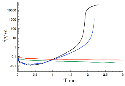
Figure 18.— Similar figure as Fig. 1 but for perpendicular magnetic fields. The solid lines represent a hydrodynamical (black), $\beta=10$ (blue), 1 (red) and 0.1 (green) model. The unit of time for our default layer is 4.9Myr.

5. Perpendicular magnetic field

The previous section discusses the gravitational instability in a layer threaded by a parallel magnetic field. Here, we examine the fragmentation for a magnetic field perpendicular to the layer. Nakano & Nakamura (1978) study the marginally stable modes of an isothermal layer with perpendicular magnetic field. They find that the layer is unstable to gravitational perturbations when $\Sigma_{0}/B_{0}>(\pi G)^{-1/2}$ or simply $\beta>1$, with the critical wavelength close to the hydrodynamical value. This means that, contrary to a parallel magnetic field, a perpendicular magnetic field can stabilize the layer as long as it is strong enough. Figure 18 indeed shows that perturbations in models with $\beta\leq 1$ are damped. For these layers to become unstable, the magnetic support needs to disappear by e.g. ambipolar diffusion (Kudoh et al., 2007; Kudoh & Basu, 2008).

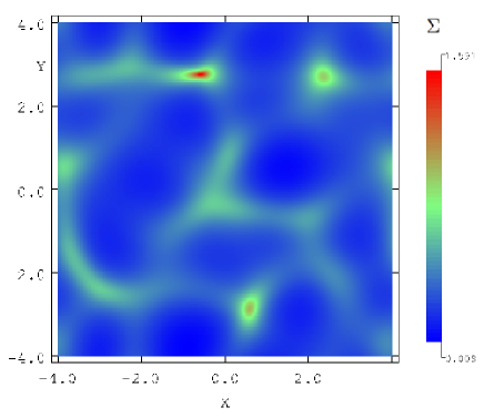
Figure 19.— Column density structure along the $z$-axis at $t=2.15$ for a perpendicular magnetic field with $\beta=10$. For the default layer, the unit of column density is 5$\times 10^{20}~{}{\rm cm^{-2}}$.

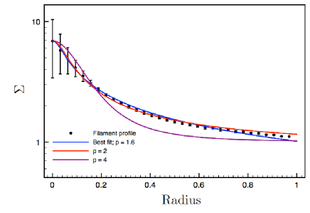
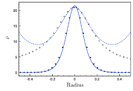
Figure 20.— Top: Average column density profile of a selected filament in Fig. 19. The error bars represent the dispersion on the average value at a given radius. The solid lines are the best-fit (blue), a $p=2$ and $p=4$ Plummer profile. The unit of column density of the default layer is 5$\times 10^{20}~{}{\rm cm^{-2}}$ and the unit of length is 1 pc. Bottom: Density profile along the $x$ (open circles) and $z$-axis (solid circles) for a slice through the filament. The blue lines show the Schmid-Burgk profile with $A=0.29$ and $\rho_{c}=11.81$ along the $x$ (dashed) and $z$ (solid) axis. For the default layer, the unit of length is 159.2 cm^-3.

Density structure and filaments

The $\beta=10$ model has a similar, though slightly slower, growth rate as the hydrodynamical model. This reduced growth rate is due to magnetic tension forces acting to straighten field lines (which are bended because the flow in the layer is perpendicular to the field lines). The mode associated with this growth still has a wavelength close to $\lambda_{\rm max}=4\pi H$, as the resulting column density structure is very similar to the hydrodynamical model (see Fig. 19). The filament ridges are actually in the same places.

Not only does the column density structure look very similar, the column density and density profiles of the filaments show the same properties as in the previous models (see Fig. 20). The power index of the best-fit Plummer profile has a value of $\leq 2$, but, at the same time, the central density structure of the filaments is perfectly described by an equilibrium Schmid-Burgk profile. Again, this means that the magnetic field only contributes marginally to the dynamics. The plasma $\beta$ near the center of the filament decreases but is still above $\beta=1$.

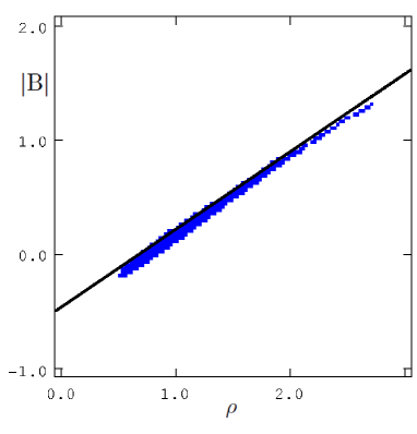
Figure 21.— Log-log relation between magnetic field magnitude and density at the midplane for the perpendicular $\beta=10$ model. The solid line shows the dependence for an isotropically contracting sphere. In terms of the default layer, the units of the magnetic field and density are given by 1.76$\mu$G and 152.9 cm^-3.

Dense cores

While the magnetic field does not influence filaments to any significant degree, the evolution of the cores are affected by them. Dense cores still arise at the junctions of the filaments, but the density distribution of the cores is very much axisymmetric. In the hydrodynamical model, gas is predominantly fed to the cores along the filaments and not isotropic as suggested here. Because of magnetic tension forces, gas in the vicinity of the cores flows directly towards the core instead of first to a filament and then towards the core. The former produces a magnetic field that is less ‘twisted’. The axisymmetry of the dense core is also observed in the scaling relation of the magnetic field and density relation, i.e. $|B|\propto\rho^{2/3}$ (see Fig. 21). Such a relation is obtained for an isotropically contracting sphere threaded by a frozen-in magnetic field. Although the magnetic energy increases more rapidly than the thermal pressure in the core (i.e. $\beta\propto\rho^{-1/3}$), the magnetic field is never strong enough to prevent collapse. The potential energy of a spherical core increases at the same rate as the magnetic energy during contraction. Initially, the gravitational energy is larger than the magnetic energy and thus remains so during the subsequent evolution.

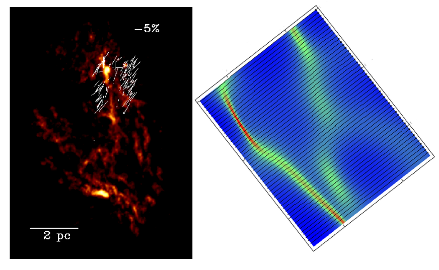
Figure 22.— Left: NH₃ emission map of the massive star forming complex G14.225-0.506 (Busquet et al., 2013). The white lines show the polarization vectors of the near-infrared (H-band) polarimetric observations (Busquet et al., 2013). Right: Section of the bottom panel of Fig. 12. The solid lines represent the mass-weighted magnetic field integrated along the $z$-axis.

6. Comparison with the star-forming region G14.225-0.506

Recently, Busquet et al. (2013) reported VLA observations in NH₃ of a massive star forming complex G14.225-0.506. The NH₃ emission reveals a network of filaments that are aligned in parallel in projection on to the plane of the sky (see Fig. 22). The filaments appear to take two directions, one group is oriented at a position angle (PA) of 10^∘, and the other is at a PA of 60^∘. The averaged projected separation between the adjacent filaments are between 0.5 pc and 1 pc. Polarimetric observations in the near infrared H-band toward the northern section of the complex reveal magnetic field orientations perpendicular to the main axis of the filaments.

The fragmentation of a layer threaded with a strong parallel magnetic field reproduces the G14.225-0.506 filament network (see Fig. 22). This allows to infer the initial conditions of the initial, unperturbed layer. The separation of the adjacent filaments is given by $\lambda_{\rm max}=4\pi H$ which results in a scale height of 0.04-0.08 pc for the unperturbed layer. Then the initial surface density is $\Sigma=a^{2}/(\pi GH)\approx 1.5-3\times 10^{-2}{\rm g\ cm^{-2}}$ (assuming a sound speed of 0.2 ${\rm km\ s^{-1}}$). As the area covered by the filaments is 4.7$\times$ 8.7 pc², the unpertubed layer contains about 2900-5800 M_☉. This agrees well with the combined mass of 2600 M_☉ for the filaments in G14.225-0.506 (Busquet et al., 2013). Also, an estimate of the magnetic field strength can be made. For the strong parallel field model, $\beta<1$ and the required magnetic field is stronger than 12-25 $\mu$G. Zeeman measurements of the magnetic field indicate that these values are towards the high end of, but within, the observed range in magnetic field strengths (Crutcher, 2012).

The initial conditions needed to produce the density structure of the filamentary complex G14.225-0.506 by gravitational instability in the presence of a strong magnetic field are not unrealistic. However, we cannot exclude any other formation process such as e.g. colliding flows.

7. Discussion and conclusions

In this paper we have examined the gravitational instability in an isothermal equilibrium layer threaded by a magnetic field. Our main results are as follows.

1. An equilibrium isothermal layer threaded by parallel magnetic fields is always unstable for gravitational instabilities with wavelengths larger than $\lambda_{\rm crit}=2\pi H$. For perpendicular magnetic fields instabilities only arise when $\beta>1$. The density structures of the unstable layer can be described by two different regimes, i.e. a hydrodynamical one and a strong magnetic one. The network structure of filaments can then be used to estimate the magnitude of the magnetic field. Parallel filaments indicate that the magnetic field is strong with $\beta\leq 1$ and that the field lines lie within the plane of the layer. On the other hand, a filament-hub structure implies that the magnetic field is weak with $\beta\gg 1$. In this case there is no connection between filament axes and the magnetic field, i.e. the magnetic field can lie parallel or perpendicular along the filament axes.

2. The filaments that form have a line-mass that exceeds the critical value for axisymmetric collapse and thus cannot be in hydrostatic equilibrium. However, at any time during their evolution, the central regions of the filaments are described by an equilibrium density structure. Using a Schmid-Burgk (1967) density profile (Eq. 5), the evolution of a filament from a perturbation in the equilibrium layer ($A\approx 0$) towards an Ostriker (1964) distribution ($A=1$) is perfectly captured. Furthermore, because of the thermal support in the central region of the filament, the collapse time is much longer than the free-fall time scale (similar to the results of Inutsuka & Miyama (1992) for collapsing cylinders).

   Although the central region of filaments is well described by equilibrium profiles, the distribution for radii above the scale height deviates from the equilibrium (as that region contains an excess of mass). The profile is then flatter than the expected power law of $r^{-4}$ and similar to the results from Herschel observations (e.g. Arzoumanian et al., 2011). An additional flattening of the profile is obtained by averaging the column density profile along a filament with a central density variation. An increase in the central density produces a larger central column density but also implies a smaller scale height (i.e. $R_{0}\propto\rho^{-1/2}$). Such a variation in the filament width is actually observed along the L1506 filament in the Taurus molecular complex (Ysard et al., 2013).

   By studying colliding flows, Gomez & Vazquez-Semadeni (2013) show that filaments also form due to dynamical and thermal instabilities in an initially sheet-like structure. While their filaments exhibit the flat column density profile of the observations and our simulations, their formation and evolution does not follow quasi-equilibrium states. Gomez & Vazquez-Semadeni (2013) argue that the filaments are just long-lived, persistent features of the flow. However, the resolution of their simulation is not high enough to resolve the thermal scale height associated with the filaments (e.g. H $\approx$ 0.3 pc for their filament 1, while the resolution is $\approx 0.17$ pc). Without the proper resolution, thermal pressure forces cannot balance gravity numerically. We encounter the same problem when we analyze filaments with a too high central density ($\rho_{c}>150$ in code units). We also recognize the difficulty in resolving the thermal scale height in turbulent simulations where the density contrasts fluctuate rapidly.

3. Our simulations do not reproduce the other property of filaments, i.e. a near constant FWHM of $\sim 0.1$ pc. As the central density of the filaments increases, the scale height continues to decrease. As the scale height also depends on pressure support, i.e. $R_{0}\propto a$, the pressure support within the filament needs to increase as it is collapsing. Our simulations show that the magnetic fields are not able to provide this extra support.

   However, Klessen & Hennebelle (2010) show that turbulence can be driven by accretion. Interstellar filaments indeed show that the filament velocity dispersion increases with column density and exceeds the thermal sound speed if they have a line-mass above the critical value (Arzoumanian et al., 2013).

4. Different authors (e.g. Li et al., 2004; Banerjee et al., 2009; Collins et al., 2011) show that the magnetic field does not prevent the formation and collapse of dense structures in molecular clouds. However, these studies only consider a low level of magnetization. In case of a strong magnetic field, simulations show that the field dominates turbulence and inhibits the gravitational collapse (e.g. Nakamura & Li, 2008; Basu & Dapp, 2010). The filaments in our simulations are purely hydrodynamical structures. This means that the magnetic field does not play a significant role in setting the shape of the filaments, even in a low-beta plasma.

5. Dense cores form at the same time as the filaments. In the hydrodynamical regime, the cores arise at the junctions of the filaments. Mass accretion of the cores depends on the orientation of the magnetic field, i.e. for perpendicular fields the accretion is roughly isotropic, while, for parallel fields, much of the gas is fed along the filaments and thus highly directional. Such non-isotropic mass accretion drastically changes the observational signatures of dense core collapse (e.g. Smith et al., 2012, 2013). Enough mass is accreted for the cores to contract, but at rates slower than free-fall collapse. This again suggests that thermal pressure (and magnetic pressure to a lesser degree) are able to roughly balance against self-gravity.

Some caveats need to be taken into account when discussing these findings. Turbulent motions are ubiquitous in the ISM and it is unlikely that a thick, quiescent equilibrium layers forms out of such a medium. For example, simulations of colliding flows (e.g. Vázquez-Semadeni et al., 2003; Audit & Hennebelle, 2005; Heitsch et al., 2008) show that the shock-bounded layer is prone to dynamical instabilities, such as Kelvin-Helmholtz and Raleigh-Taylor instabilities, but also to thermal instabilities. However, Kudoh & Basu (2011) show that, dense core profiles do not not depend strongly on the initial velocity perturbations, although their formation time scales are shorter for larger velocity fluctuations.

For a thin isothermal layer, the nature of the gravitational instability changes and is very similar to an incompressible mode. Nagai et al. (1998) show that the density perturbations are then a result of a deformation of the boundary of the layer. When the layer is threaded by a strong magnetic field ($\beta<1$), filaments no longer form perpendicular to the magnetic field lines but parallel to them. Furthermore, the line-mass of the filaments is smaller than the critical value. Then the filaments do not longer collapse but are in equilibrium. It is then expected that the filament fragments along its axis into cores with equal spacing between them. We will study this possibility in a subsequent paper.

References

- Alves et al. (2001) Alves, J. F., Lada, C. J., & Lada, E. A. 2001, Nature, 409, 159
- André et al. (2010) André, P., Men’shchikov, A., Bontemps, et al. 2010, A&A, 518, L102+
- Arzoumanian et al. (2011) Arzoumanian, D., André, P., Didelon, P., et al. 2011, A&A, 529, L6+
- Arzoumanian et al. (2013) Arzoumanian, D., André, P., Peretto, N., Konyves, V. 2013, A&A, 553, A119
- Audit & Hennebelle (2005) Audit, E., & Hennebelle, P. 2005, A&A, 433, 1
- Ballesteros-Paredes et al. (1999) Ballesteros-Paredes, J., Hartmann, L., & Vázquez-Semadeni, E. 1999, ApJ, 527, 285
- Ballesteros-Paredes & Mac Low (2002) Ballesteros-Paredes, J., & Mac Low, M.-M. 2002, ApJ, 570, 734
- Ballesteros-Paredes et al. (2007) Ballesteros-Paredes, J., Klessen, R. S., Mac Low, M.-M., & Vazquez-Semadeni, E. 2007, Protostars and Planets V, 63
- Banerjee et al. (2009) Banerjee, R., Vázquez-Semadeni, E., Hennebelle, P., & Klessen, R. S. 2009, MNRAS, 398, 1082
- Basu & Dapp (2010) Basu, S., & Dapp, W. B. 2010, ApJ, 716, 427
- Bonnor (1956) Bonnor, W. B. 1956, MNRAS, 116, 351
- Busquet et al. (2013) Busquet, G., Zhang, Q., Palau, A., et al. 2013, ApJ, 764, L26
- Collins et al. (2011) Collins, D. C., Padoan, P., Norman, M. L., & Xu, H. 2011, ApJ, 731, 59
- Crutcher (2012) Crutcher, R. M. 2012, ARA&A, 50, 29
- Curry (2000) Curry, C. L. 2000, ApJ, 541, 831
- de Avillez & Breitschwerdt (2005) de Avillez, M. A., & Breitschwerdt, D. 2005, A&A, 436, 585
- Dedner et al. (2002) Dedner, A., Kemm, F., Kröner, D., et al. 2002, Journal of Computational Physics, 175, 645
- Elmegreen & Elmegreen (1978) Elmegreen, B. G., & Elmegreen, D. M. 1978, ApJ, 220, 1051
- Falle (1991) Falle S. A. E. G., 1991, MNRAS, 250, 581
- Falle et al. (2012) Falle, S., Hubber, D., Goodwin, S., & Boley, A. 2012, Numerical Modeling of Space Plasma Slows (ASTRONUM 2011), 459, 298
- Fiege & Pudritz (2000) Fiege, J. D., & Pudritz, R. E. 2000, MNRAS, 311, 105
- Fischera & Martin (2012) Fischera, J., & Martin, P. G. 2012, A&A, 542, A77
- Galván-Madrid et al. (2013) Galván-Madrid, R., Liu, H. B., Zhang, Z.-Y., et al. 2013, ApJ, 779, 121
- Goldsmith et al. (2008) Goldsmith, P., Heyer, M., Narayanan, G., Snell, R., Li, D., & Brunt, C. 2008, ApJ, 680, 428
- Gomez & Vazquez-Semadeni (2013) Gomez, G. C., & Vazquez-Semadeni, E. 2013, arXiv:1308.6298
- Goodman et al. (1990) Goodman, A. A., Bastien, P., Myers, P. C., & Ménard, F. 1990, ApJ, 359, 363
- Goodman et al. (1992) Goodman, A. A., Jones, J. T., Lada, E. A., & Myers, P. C. 1992, ApJ, 399, 108
- Heitsch (2013) Heitsch, F. 2013, ApJ, 769, 115
- Heitsch et al. (2008) Heitsch, F., Hartmann, L. W., & Burkert, A. 2008, ApJ, 683, 786
- Inutsuka & Miyama (1992) Inutsuka, S., & Miyama, S. M. 1992, ApJ, 388, 392
- Johnstone & Bally (1999) Johnstone, D., & Bally, J. 1999, ApJ, 510, L49
- Keto et al. (2004) Keto, E., Rybicki, G. B., Bergin, E. A., & Plume, R. 2004, ApJ, 613, 355
- Kirk et al. (2013) Kirk, H., Myers, P. C., Bourke, T. L., et al. 2013, ApJ, 766, 115
- Klessen & Hennebelle (2010) Klessen, R. S., & Hennebelle, P. 2010, A&A, 520, A17
- Koyama & Inutsuka (2000) Koyama, H., & Inutsuka, S.-I. 2000, ApJ, 532, 980
- Kudoh et al. (2007) Kudoh, T., Basu, S., Ogata, Y., & Yabe, T. 2007, MNRAS, 380, 499
- Kudoh & Basu (2008) Kudoh, T., & Basu, S. 2008, ApJ, 679, L97
- Kudoh & Basu (2011) Kudoh, T., & Basu, S. 2011, ApJ, 728, 123
- Ledoux (1951) Ledoux, P. 1951, Annales d’Astrophysique, 14, 438
- Li et al. (2004) Li, P. S., Norman, M. L., Mac Low, M.-M., & Heitsch, F. 2004, ApJ, 605, 800
- Li et al. (2013) Li, H.-b., Fang, M., Henning, T., & Kainulainen, J. 2013, MNRAS, 2585
- Liu et al. (2012) Liu, H. B., Jiménez-Serra, I., Ho, P. T. P., et al. 2012, ApJ, 756, 10
- Lindeberg (1998) Lindeberg, T. 1998, International Journal of Computer Vision, 30, 117
- Men’shchikov et al. (2010) Men’shchikov, A., André, P., Didelon, P., et al. 2010, A&A, 518, L103+
- Molinari et al. (2011) Molinari, S., Bally, J., Noriega-Crespo, A., et al. 2011, ApJ, 735, L33
- Myers (1983) Myers, P. C. 1983, ApJ, 270, 105
- Myers (2009) Myers, P. C. 2009, ApJ, 700, 1609
- Miyama et al. (1987) Miyama, S. M., Narita, S., & Hayashi, C. 1987, Progress of Theoretical Physics, 78, 1273
- Mizuno et al. (1995) Mizuno, A., Onishi, T., Yonekura, Y., Nagahama, T., Ogawa, H., & Fukui, Y. 1995, ApJ, 445, 161
- Nagai et al. (1998) Nagai, T., Inutsuka, S.-I., & Miyama, S. M. 1998, ApJ, 506, 306
- Nakajima & Hanawa (1996) Nakajima, Y., & Hanawa, T. 1996, ApJ, 467, 321
- Nakamura & Li (2008) Nakamura, F., & Li, Z.-Y. 2008, ApJ, 687, 354
- Nakano & Nakamura (1978) Nakano, T., & Nakamura, T. 1978, PASJ, 30, 671
- Ostriker (1964) Ostriker, J. 1964, ApJ, 140, 1056
- Padoan & Nordlund (2002) Padoan, P., & Nordlund, Å. 2002, ApJ, 576, 870
- Palmeirim et al. (2013) Palmeirim, P., André, P., Kirk, J., et al. 2013, A&A, 550, A38
- Peretto et al. (2012) Peretto, N., André, P., Könyves, V., et al. 2012, A&A, 541, A63
- Pon et al. (2012) Pon, A., Toalá, J. A., Johnstone, D., et al. 2012, ApJ, 756, 145
- Schmid-Burgk (1967) Schmid-Burgk, J. 1967, ApJ, 149, 727
- Schneider & Elmegreen (1979) Schneider, S., & Elmegreen, B. 1979, ApJS, 41, 87
- Schneider et al. (2012) Schneider, N., Csengeri, T., Hennemann, M., et al. 2012, A&A, 540, L11
- Smith et al. (2012) Smith, R. J., Shetty, R., Stutz, A. M., & Klessen, R. S. 2012, ApJ, 750, 64
- Smith et al. (2013) Smith, R. J., Shetty, R., Beuther, H., Klessen, R. S., & Bonnell, I. A. 2013, ApJ, 771, 24
- Spitzer (1942) Spitzer, L., Jr. 1942, ApJ, 95, 329
- Tafalla et al. (2004) Tafalla, M., Myers, P. C., Caselli, P., & Walmsley, C. M. 2004, A&A, 416, 191
- Toalá et al. (2012) Toalá, J. A., Vázquez-Semadeni, E., & Gómez, G. C. 2012, ApJ, 744, 190
- Truelove et al. (1997) Truelove, J. K., Klein, R. I., McKee, C. F., et al. 1997, ApJ, 489, L179
- Umekawa et al. (1999) Umekawa, M., Matsumoto, R., Miyaji, S., & Yoshida, T. 1999, PASJ, 51, 625
- Van Loo et al. (2006) van Loo S., Falle S. A. E. G., Hartquist T. W., 2006, MNRAS, 370, 975
- van Loo et al. (2007) van Loo, S., Falle, S. A. E. G., Hartquist, T. W., & Moore, T. J. T. 2007, A&A, 471, 213
- van Loo et al. (2010) van Loo, S., Falle, S. A. E. G., & Hartquist, T. W. 2010, MNRAS, 406, 1260
- Vázquez-Semadeni et al. (2003) Vázquez-Semadeni, E., Ballesteros-Paredes, J., & Klessen, R. S. 2003, ApJ, 585, L131
- Ysard et al. (2013) Ysard, N., Abergel, A., Ristorcelli, I., et al. 2013, arXiv:1309.6489