A Strict Test of Stellar Evolution Models: The Absolute Dimensions of Massive Benchmark Eclipsing Binary V578 Mon

Abstract

We determine the absolute dimensions of the eclipsing binary V578 Mon, a detached system of two early B-type stars (B0V + B1V, P$=$2.40848 d) in the star-forming region NGC 2244 of the Rosette Nebula. From the light curve analysis of 40 yr of photometry and the analysis of hermes spectra, we find radii of $5.41\pm 0.04$ Rsun and $4.29\pm 0.05$ Rsun, and temperatures of $30000\pm 500$ K and $25750\pm 435$ K respectively. We find that our disentangled component spectra for V578 Mon agree well previous spectral disentangling from the literature. We also reconfirm the previous spectroscopic orbit of V578 Mon finding that masses of $14.54\pm 0.08$ Msun and $10.29\pm 0.06$ Msun are fully compatible with the new analysis. We compare the absolute dimensions to the rotating models of the Geneva and Utrecht groups and the models of Granada group. We find all three sets of models marginally reproduce the absolute dimensions of both stars with a common age within uncertainty for gravity-effective temperature isochrones. However - there are some apparent age discrepancies for the corresponding mass-radius isochrones. Models with larger convective overshoot $>0.35$ worked best. Combined with our previously determined apsidal motion of $0.07089^{+0.00021}_{-0.00013}$ deg cycle^-1, we compute the internal structure constants (tidal Love number) for the newtonian and general relativistic contribution to the apsidal motion, $\log{k_{2}}=-1.975\pm 0.017$ and $\log{k_{2}}=-3.412\pm 0.018$ respectively. We find the relativistic contribution to the apsidal motion of be small $<4\%$. We find that the prediction of $\log{k_{\rm 2,theo}}=-2.005\pm 0.025$ of the Granada models fully agrees with our observed $\log{k_{2}}$.

1 Introduction

Detached eclipsing binary stars (dEBs) provide accurate observed stellar masses, radii, effective temperatures, and rotational velocities. See a recent review by Torres et al. (2010) for a discussion of 94 dEBs with accurate masses and radii used to test stellar evolution models. There are only nine total massive dEBs, or equivalently 18 stars whose physical parameters have been determined with an accuracy of better than 3%, making V578 Mon one of only nine EBs with $M_{1}\geq M_{2}>10$ $\mbox{M}_{\mbox{$\odot$}}$ and with sufficient accuracy to be included in the Torres et al. (2010) compilation of benchmark-grade EBs. Figure 1 demonstrates the upper main sequence of all dEBs with $M_{1}\geq M_{2}>10$ $\mbox{M}_{\mbox{$\odot$}}$ and masses and radii determined to 3% (adapted from Torres et al. (2010)). V578 Mon is therefore a benchmark system for testing stellar evolution models of newly formed massive stars. The accurate absolute dimensions of eclipsing binary stars provide a unique opportunity to test stellar evolution models in two ways: the “isochrone test” and the“apsidal motion test”.

The “isochrone test” of stellar evolution models requires that the ages of both components of a dEB predicted from separate stellar evolution tracks to be the same within uncertainty of the absolute dimensions $(M,R,T_{\rm eff},v_{\rm rot})$. For the “isochrone test”, we assume that both components of the dEB formed together in the same initial gas cloud. Therefore, both components of a dEB are assumed to arrive at the zero age main sequence (ZAMS) at nearly the same time. Furthermore, their initial chemical compositions must be the same. Finally, we assume that each component of the binary evolves in isolation, where the effects of the companion star on the evolution is small or negligible.

The “isochrone test” is strongest for eclipsing binaries with low mass ratios $q=\frac{M_{2}}{M_{1}}<1$. For dEBs where component masses $M_{1}\approx M_{2}$, both stars will evolve on the same evolutionary track. This does not allow for strict tests of stellar evolution models unless the chemical composition or effective temperature of the stars is known. Stellar evolution models will predict two stars of the same mass and composition to have the same age. Conversely, the larger the difference in initial mass between the components of the binary star, the larger the difference in main sequence (MS) lifetimes of the two stars. Therefore, the stellar models must have the accurate input physics to correctly predict how quickly stars of different mass evolve relative to each other. The correct input physics in turn yields correct predictions of the observed absolute dimensions of the detached eclipsing binary.

Detached eclipsing binary stars with apsidal motion (precession of the argument of periastron) also allow for the “apsidal motion test” of the stellar internal structure (Claret & Giménez 2010). Physically, the observed apsidal motion rate in an eclipsing binary is a result of the tidal forces of each star on each other. In turn, this tidal force is linked to the internal structure of each star, the star’s separation, their mass ratio $q$ and their radii $R_{1}$ and $R_{2}$. The internal structure is quantified by the constant $\log{k_{2}}$ which is the logarithm of twice the tidal Love number (Kramm et al. 2011). The “apsidal motion” test compares the theoretical internal structure constant $\log{k_{\rm 2,theo}}$ to the observed internal structure constant $\log{k_{\rm 2,obs}}$. The observed internal structure constant is a function the observed absolute dimensions and apsidal motion of the eclipsing binary. The observed internal structure constant is very sensitive to the radii ($k_{\rm 2,obs}\propto R^{5}$) - therefore, this test can only be performed with accurate stellar radii. However, including this study of massive dEB V578 Mon, there are only five massive, eccentric eclipsing binaries available for these tests of internal structure (Claret & Giménez 2010).

Here we combine the previous determination of $\dot{\omega}$ and $e$ from Garcia et al. (2011) with a reanalysis of 40 years worth of photometry to re-determine the fundamental properties of V578 Mon. We include the photometry used by the previous light curve analysis (Hensberge et al. 2000). We compare the masses, temperatures and radii of V578 Mon with rotating high mass stellar evolution models by Granada (Claret 2004, 2006), Geneva (Georgy et al. 2013; Ekström et al. 2012), and Utrecht (Brott et al. 2011) groups. We also compare the observed internal structure constant $\log{k_{\rm 2,obs}}$ with theoretical $\log{k_{\rm 2,theo}}$ using the methods of Claret & Giménez (2010).

2 The Eclipsing Binary V578 Mon in NGC 2244

The photometric variability of the bright (V=8.5), 2.408 day period, eccentric, massive detached eclipsing binary (dEB) V578 Mon (HDE 259135, BD$+4^{\circ}$1299), comprising a B1V type primary star and a B2V type secondary star was first identified in the study by Heiser (1977) of NGC 2244 within the Rosette Nebula (NGC 2237, NGC 2246). The identifications, locations and photometric parameters for V578 Mon are listed in Table 1. The absolute dimensions of V578 Mon have been determined from three seasons of Strömgren $uvby$ photometry and one season of radial-velocity data by Hensberge et al. (2000). An analysis of the metallicity and evolutionary status of V578 Mon was undertaken by Pavlovski & Hensberge (2005) and Hensberge et al. (2000). The masses and radii of V578 Mon determined from these data are $14.54\pm 0.08$ $\mbox{M}_{\mbox{$\odot$}}$ and $10.29\pm 0.06$ $\mbox{M}_{\mbox{$\odot$}}$, and $5.23\pm 0.06$ $\mbox{R}_{\mbox{$\odot$}}$ and $4.32\pm 0.07$ $\mbox{R}_{\mbox{$\odot$}}$  for the primary and secondary respectively (Hensberge et al. 2000). V578 Mon was included in the list of 94 detached eclipsing binaries with masses and radii accurate to $2\%$ by Torres et al. (2010). The radii for V578 Mon listed in Torres et al. (2010) were found to be incorrect by Garcia et al. (2013) given system’s eccentric orbit and asynchronous rotation. The apsidal motion $\dot{\omega}$ and a new eccentricity $e$ were determined in Garcia et al. (2011). V578 Mon was observed by MOST (Pribulla et al. 2010).

Given the inclination of V578 Mon, its eclipses are partial, meaning that neither star is fully out of view of Earth. Partial eclipses can translate into a degeneracy between the radii, preventing the component radii $R_{1}$ and $R_{2}$ from being individually measured. However, V578 Mon also has an eccentric orbit, meaning that the eclipse durations are not equal, which helps breaks this degeneracy and allows the radii to be determined separately. V578 Mon is observed to not have tidally locked yet. The system has a low mass ratio $q$=$0.7078$ as compared to similar systems with well-determined absolute parameters such as V1034 Sco, V478 Cyg, AH Cep, V453 Cyg, and CW Cep (Bouzid et al. 2005; Popper & Etzel 1981; Popper & Hill 1991; Bell et al. 1986; Holmgren et al. 1990; Southworth et al. 2004; Popper 1974; Stickland et al. 1992). Of all of these systems, V578 Mon is also the youngest, making this system a benchmark case for testing stellar evolution models at the youngest ages.

3 Data

3.1 Johnson UBV and Strömgren $uvby$ Photometry

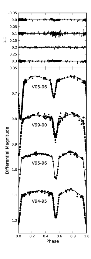
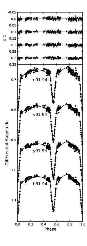
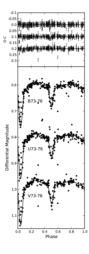
The available time-series photometry of V578 Mon covers nearly 40 yr and more than one full apsidal motion period. A summary of the various light curve epochs, including filters and observing facilities used, is presented in Table 2. Photometry from Heiser (2010) includes multi-band light curves spanning 1967–2006 from the 16-in telescope at Kitt Peak National Observatory (KPNO) and from the Tennessee State University(TSU) -Vanderbilt 16-in Automatic Photoelectric Telescope (APT) at Fairborn Observatory. The KPNO Johnson $UBV$ light curves comprise 725 data points spanning 1967–1984 with average uncertainties per data point of 0.004 mag computed by Heiser (2010). The APT Johnson $BV$ light curves span 1994–2006 and consist of 1783 data points with average uncertainties per data point of 0.001 mag for B and 0.002 mag for V (Heiser 2010). Light curves from Hensberge et al. (2000) span 1991–1994 from the 0.5-m Strömgren Automatic Telescope (SAT) at La Silla, with 248 data points in each of the $uvby$ filters and average uncertainty per data point of 0.003 mag (Hensberge et al. 2000). We begin our light curve analysis with the observational errors originally estimated by Heiser (2010) and Hensberge et al. (2000). Table 2 lists these average uncertainties, $\sigma_{0}$, as reported by the original authors. However, from our light curve fits (see below) we found that these uncertainties were in most cases underestimated. Thus we also report as $\sigma$ in Table 2 the uncertainties that we ultimately adopted for each light curve.

3.2 hermes Spectroscopy

A new series of high-resolution echelle spectra were secured in December 2011 (36 exposures) and February 2012 (8 exposures) with hermes, the fiber-fed high-resolution spectrograph on the Mercator telescope located at the Observatorio del Roque de los Muchachos, La Palma, Canary Islands. hermes samples the entire optical wavelength range (3800-9000 Å) with a resolution of $R=85\,000$ (Raskin et al. 2011). The observations listed in Table 3 cover the orbital cycle uniformly. Groups of two concatenated exposures allow us to obtain a robust estimation of random noise as a function of wavelength, and a check on cosmic ray events surviving the detection algorithm in the data reduction. In total, 44 exposures were obtained at 19 epochs, 16 of which are out of eclipse. One series of six exposures starts near the primary mid-eclipse; One series of two concatenated exposures taken around secondary mid-eclipse has a significantly lower exposure level, but another one consisting of four concatenated exposures starting around secondary mid-eclipse is available.

Exposure times close to 2100 s were used for most spectra, but in case of one out-of-eclipse epoch the exposure time was significantly shorter, 1200 s. The signal-to-noise ratio of the spectra is 50 to 100 at 4000 Å, then rapidly increasing to 120 up to 200 at 5000 Å and remaining close to this level at longer wavelengths. The numbers apply to the sum of two concatenated exposures. The reduction of the spectra has been performed using the heres pipe-line software package. The spectra resampled directly in constant-size velocity bins (ln $\lambda$), very nearly in size to the detector pixels, were used. Normalization to the continuum is done separately.

The hermes spectra outnumber the caspec spectra used by Hensberge et al.(̃2000), but fall short with regard to signal-to-noise ratio. However, they cover a much larger wavelength region, include epochs in both eclipses and cover the orbit more homogeneously. In the wavelength region covered by both sets, the reconstruction has better signal-to-noise ratio in the caspec set, but the risk of bias due to phase gaps might be higher with the caspec data. Both data sets were obtained in different parts of the apsidal motion cycle.

4 Analysis

4.1 Spectral Disentangling & Light Ratio

In V578 Mon binary system the eclipses are partial which causes degeneracy in the light curve solution for the radii of the components. It was checked whether a spectroscopic light ratio has sufficient precision to reduce the degeneracy. This light ratio might be constrained either by the changing line dilution during the eclipse, or/and by constrained fitting of the reconstructed component spectra by theoretical spectra, simultaneously deriving the light ratio as well as the photospheric parameters (Tamajo et al. 2011). In the latter implementation, the light ratio is assumed identical in all observed spectra, hence eclipse spectra are not used.

With partial eclipses of roughly 0.1 mag depth, and less for the secondary eclipse at the epoch of the spectroscopy, line depth in the composite spectrum is affected at the level of 0.5% of the continuum only when the two components have in their intrinsic spectra a line differing by 7% of the continuum depth. The similarity of the components and the rotational broadening in the spectra imply that no metal line approaches this level. Hence, using the changing line dilution to measure the light ratio precisely is challenging. Exceedingly large signal-to-noise ratios would be required to be able to use single or few lines. Including many lines, i.e. large stretches of spectrum offers the opportunity to reduce the requirements on the signal-to-noise ratio. However, bias in tracing the continuum is expected to put an upper limit to the precision with which the light ratio can be measured in a system with components with similar spectra and substantial rotation.

Therefore, we explored the alternative option of constrained fitting, although it is model-sensitive. Spectral disentangling (Hadrava 1995), further referred as spd is performed in a spectral range of about 100 - 150 Å (of the order of 4000 bins) in the wavelength range 3900 - 5000 Å, centered on prominent lines of He i, He ii and stronger metal lines. The apsidal motion study (Garcia et al. 2011) permitted us to fix the eccentricity $e$, the longitude of the periastron, $\omega$, for the epoch of the spectra, and the time of periastron passage. The spd code used is FDBinary (Ilijic et al. 2004).

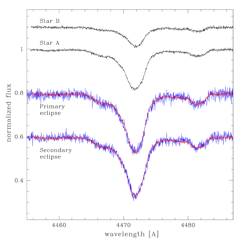
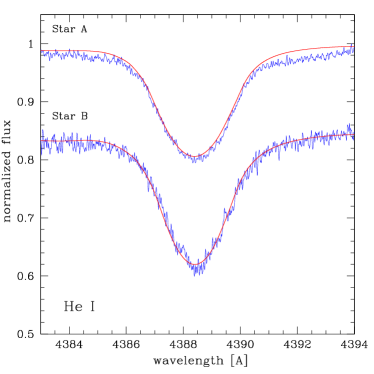
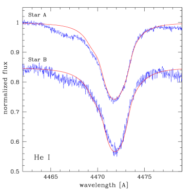
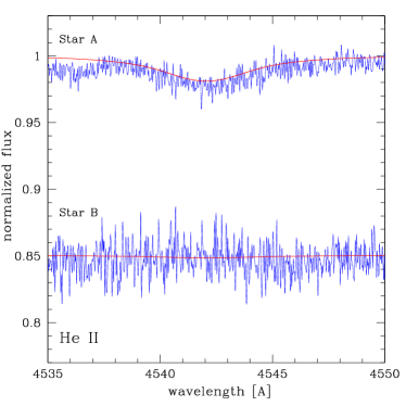
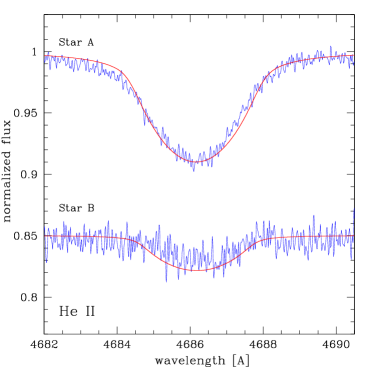
spd applied to selected spectral regions of the hermes spectra, well distributed over the full range of Doppler shifts in the orbit (see orbital phases in Table 3), leads to radial velocity amplitudes K1 and K2 compatible with Hensberge et al. (2000) within better than 1 km/s. Thus the spectra are reconstructed using the mean orbital elements (Table 4), now also including regions around $H_{\gamma}$ and H_δ ($H_{\beta}$ has a broad interstellar band centered on its red wing). For the constrained fitting, optimization was done for hydrogen and helium lines only, and for combinations of them. The reconstructed spectra for both out-of-eclipse and in-eclipse phases are shown in Figures 2 and 3.

The component spectra for different dilution factors can be obtained from a single disentangling computation, followed by an adequate renormalisation. As starting point for the photospheric parameters, $T_{\rm eff,1}=30\,000$ K, and $T_{\rm eff,2}=26\,400$ K is used, based on the extensive study of Hensberge et al. (2000) and Pavlovski & Hensberge (2005). The surface gravities of the components are fixed to $\log{g_{\rm 1}}$= $4.133\pm 0.018$ and $\log{g_{\rm 2}}$= $4.185\pm 0.021$ as derived in this paper. This suppresses the degeneracy of line profiles of hot stars in the (temperature, gravity) plane. Calculations for a small grid in $\log{g}$ has shown that the effect of fixing $\log{g}$ might produce deviations of about a few tenths of the percentage in determining the light dilution factors.

Optimization of relative light factors includes a search through a grid of theoretical spectra, using a genetic algorithm. A grid of synthetic spectra was calculated assuming non-LTE line formation. The calculations are based on the so-called hybrid approach of Nieva & Przybilla (2007) in which model atmospheres are calculated in LTE approximation and non-LTE spectral synthesis with detailed statistical balance. Model atmospheres are constructed with atlas9 for solar metallicity, [M/H] = 0, and helium abundance by number density, $N_{\rm He}/N_{\rm tot}=0.089$ (Castelli et al. 1997). Non-LTE level populations and model spectra were computed with recent versions of detail and surface (Butler & Giddings 1985). Further details on the method, grid and calculations can be found in Tamajo et al. (2011) and Pavlovski et al. (2009).

Depending on the line(s) included, the primary is found to contribute 68 to 72 percent of the total light, with hydrogen lines supporting the larger fractions. Hydrogen suggests a few percent lower temperature for the primary, compared to the starting values. This is compatible with the tendency seen in Figure 7 of Hensberge et al. (2000), that H and He lines for the primary only marginally agree on effective temperature (taking minimum $\chi^{2}$ at the relevant gravity, a 1000 K difference in temperature estimation occurs).

The inconsistency between different indicators underlines the importance to develop a more consistent atmosphere model for these stars. One way, following Nieva & Przybilla (2012), is to include more ionization equilibria by analyzing the full wavelength range covered by the new spectra. This work-intensive analysis is out of the scope of the present paper, but probably indispensable to constrain better the degeneracy in the determination of the radii. Its success might be limited by the rotational broadening in the spectra. Another point of attention is the need to take into account temperature and gravity variations over the surface, due to the slightly non-spherical shape of the stars. Our work shows that the purely photometrically estimated light factors (Table 5) lie within the broader range $0.68-0.72$ of light factors (primary to total light) derived here from the hermes spectra. However, there are some warnings that improvement is needed - the spectroscopic estimates may be biased as different indicators are not yet fully compatible.

4.2 Light Curve Analysis

We use EB modeling software phoebe (Prša & Zwitter 2005) based on Wilson-Devinney code (Wilson & Devinney 1971; Wilson, 1979) for our light curve analysis. We fit light curves spanning $40$ yrs, covering one full apsidal motion cycle and in Johnson $UBV$ and Strömgren $uvby$ photometry.

Figures 4, 5, 6, 7 are the residuals (data-model) for our global best fit model to the light curves for every light curve epoch and filter in Table 2. Overall, the residuals are small - typically $\approx 0.005$ mag. The residuals are significantly larger for light curve epochs 1970-1984, since error bars on the photometry data points measured using photometric plates is larger. We explore ranges for our light curve parameters as listed in Table 6. Our global best fit matches observations well - the final light curve parameters $\Omega_{1}$, $\Omega_{2}$, $i$, and $\frac{T_{2}}{T_{1}}$ are listed in Table 7.

4.2.1 Setup

For our global best fit light curve model, we adopt a square root limb darkening law (Claret 2000), a B1V spectral type for the primary star implying $T_{1}=30000$ K (Hensberge et al. 2000), no light reflection, and no third light.

We have four light curve parameters of interest - primary potential $\Omega_{1}$, secondary potential $\Omega_{2}$, inclination $i$ and temperature ratio $\frac{T_{2}}{T_{1}}$. A “parameter of interest” is defined as a parameter that is varied to compute our confidence intervals. We determine these parameters and their uncertainties by mapping $\chi^{2}$ space. Potential $\Omega$ is a modified Kopal potential for asynchronous, eccentric orbits (Wilson, 1979). The potential ($\Omega\propto R^{-1}$) takes into account contributions from the star itself, its companion, the star’s rotation about its axis, and the star’s rotation in its orbit.

Our fixed parameters are the argument of periastron $w_{0}$, eccentricity $e$, apsidal motion $\dot{\omega}$, semi-major axis $a$, mass ratio $q$, period $P$, ephemeris HJD₀, systemic velocity $\gamma$, gravity brightening coefficients $g_{1}$ & $g_{2}$, primary and secondary synchronicity parameters $F_{1}$, $F_{2}$ and albedos $A_{1}$, $A_{2}$. We fix the argument of periastron $w_{0}$, eccentricity $e$ and apsidal motion $\dot{\omega}$ to values determined by a multi-epoch light curve analysis from Garcia et al. (2011). We fix mass ratio $q\equiv\frac{M_{2}}{M_{1}}$, semi-major axis $a$, orbital period $P$, time of minima HJD₀ and systemic velocity $\gamma$ to values from Hensberge et al. (2000) analysis of the spectroscopic orbit. As mentioned previously, our hermes spectra analysis derives radial velocity amplitudes $K_{1}$ and $K_{2}$ in agreement with the Hensberge et al. (2000) spectroscopic orbit (see Table 4). We adopt gravity brightening coefficients ($g_{1},g_{2}$) and surface albedos ($A_{1},A_{2}$) to be $1.0$ as appropriate for stars with radiative envelopes. The gravity brightening coefficient $g_{1}=g_{2}=1.0$ for stars with radiative envelopes was first found by von Zeipel (1924). We fixed rotational synchronicity parameters $F_{1}=1.13$ and $F_{2}=1.11$ to values from Hensberge et al. (2000). Our limb darkening coefficients follow the square-root law for hot stars (Claret 2000) and are listed in Table 8.

4.2.2 Fitting Method

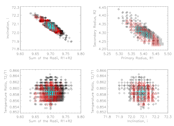
Our fitting method is adapted from Gómez Maqueo Chew et al. (2014, in prep). We determine our best fit global light curve solution by finding a unique set of light curve parameters $\Omega_{1}$, $\Omega_{2}$, $\frac{T_{2}}{T_{1}}$ and $i$ that correspond to the minimum chi square $\chi^{2}_{\rm min}$ in a well mapped grid of parameter space. The chi square is a function of the light curve parameters, $\chi^{2}=\chi^{2}(\Omega_{1},\Omega_{2},\frac{T_{2}}{T_{1}},i)$. We map parameter space by computing $\chi^{2}$ for a grid of $>10^{5}$ unique sets of these light curve parameters. We use our map of parameter space to compute the uncertainties on our light curve parameters using confidence intervals. Plots of $\Delta\chi^{2}$ vs stellar radii $R_{1}$, $R_{2}$, temperature ratio $\frac{T_{2}}{T_{1}}$, and inclination $i$ with confidence intervals are shown in Figure 8.

The step-by-step procedure is as follows:

1. We sample a coarse grid of $10^{4}$ points defined by a range of potential $\Omega_{1}$, potential $\Omega_{2}$, inclination $i$ and temperature ratio $\frac{T_{2}}{T_{1}}$. The parameter ranges and spacings are given in Table 6.

For each grid point, we fit only for the “light levels” in phoebe which is equivalent to the total light contribution from each star in the photometric bandpass. We avoid using the WD2003 differential corrections (DC) fitting algorithm within phoebe to fit our light curve parameters. The DC algorithm can fall into local minima when fitting for many parameters. We compute the total chi square $\chi^{2}_{k}$ for each light curve fit as the sum of the chi square $\chi^{2}_{p}$ at each passband and epoch:

$$\chi^{2}_{k}(\Omega_{1k},\Omega_{2k},\frac{T_{2k}}{T_{1}},i_{k})=\sum^{15}_{p}\frac{\chi^{2}_{p}}{\sigma_{p}^{2}}$$ (1)

Where index $k$ corresponds to a unique point in parameter space ($\Omega_{1k}$, $\Omega_{2k}$, $\frac{T_{2k}}{T_{1}}$, $i_{k}$). $\chi^{2}_{k}$ is the total chi square over all light curves at a unique point $k$. Index $p$ corresponds to a unique light curve passband epoch as specified in Table 2. The chi square at specific passband $\chi^{2}_{p}$ is computed as:

$$\chi^{2}_{p}=\sum^{N}_{i}\frac{(f-f_{m})^{2}}{\sigma_{i}^{2}}$$ (2)

Where $N=N_{d}-N_{p}=3485$ is the number of photometry data points $N_{d}$ minus the number of parameters of interest $N_{p}$ over all light curve epochs. Each data point has an error bar $\sigma_{i}$. Each light curve at a specific epoch and filter has a multiplicative factor $\sigma_{p}$ which takes into account systematic error. Multiplicative factor $\sigma_{p}$ is used to normalize the $\chi^{2}$ such that $\chi^{2}_{\rm min}=N$ or reduced $\chi^{2}_{\rm min,red}=1.0$. $f$ is the total flux of the binary at an HJD, and flux $f_{m}$ is the corresponding model. From our coarse grid, we find the minimum total chi square $\chi^{2}=\chi^{2}_{\rm min}$ in parameter space.

2. We adjust the error bars of the individual photometry data points for all light curves to take into account any systematic error. For the minimum $\chi^{2}_{\rm min}$ solution, the passband $\sigma_{p}$ is computed for each separate light curve epoch and filter using the equation:

$$\sigma_{p}=\sqrt{\frac{N}{\chi^{2}_{\rm min}}}$$ (3)

Where $N=3486$ as in step 1, and $\chi^{2}_{\rm min}$ is the minimum total $\chi^{2}$ of the coarse grid. We choose compute multiplicative factor $\sigma_{p}$ to weight each light curve such that the minimum reduced chi squared $\chi^{2}_{\rm min,red}=1.0$ for our global best fit solution. We then rescale the $\chi^{2}$ of all other light curve fits using the passband $\sigma_{p}$:

$$\chi^{2}_{k}=\sum^{15}_{p}\frac{\chi^{2}}{\sigma_{p}^{2}}$$ (4)

Where $\chi^{2}$ un-scaled and $\chi^{2}_{k}$ is the scaled chi square at a unique point in parameter space $k$.

3. We perform steps 1 and 2 for a fine grid of $>10^{5}$ points in parameter space around the location of the minimum $\chi^{2}_{\rm min}$. In this way we carefully map out parameter space at the location of the $\chi^{2}_{\rm min}$. We use multiple fine grids to precisely find our global best fit minimum. The average grid spacings are $0.005$, $0.005$, $0.03$ and $0.0005$ respectively for $\Omega_{1}$, $\Omega_{2}$, $i$ and $\frac{T_{2}}{T_{1}}$.

We find that the location of the minimum $\chi^{2}$ moves slightly, and we recompute the multiplicative factor $\sigma_{p}$ for each light curve to account for this, again making $\chi^{2}_{\rm min,red}=1.0$. Finally, we have a global best fit solution within a finely sampled parameter space. Our global best fit solution listed in Table 7 corresponds to the point in parameter space where scale chi square by $\sigma_{p}$ such that $\chi^{2}_{\rm min,red}=1.0$.

4.2.3 A Comparison of Light Curve Models

In order to ensure our light curve solution is robust and thus our light curve parameters are accurate, we compare our best fit light curve model described above with several other models. As shown in Table 9 we find little effect on our best fit light curve parameters from using different light curve models. All other models are not as favorable due to larger $\chi^{2}$ or temperatures that do not agree with the analysis of the component spectra of V578 Mon from spectral disentangling of Hensberge et al. (2000).

For all the tests described below, we start at our best fit solution, then fit all light curves in phoebe for primary potential $\Omega_{1}$, secondary potential $\Omega_{2}$, temperature ratio $\frac{T_{2}}{T_{1}}$, and inclination $i$. Our global best fit uses a fixed primary temperature T${}_{1}=30000$ K, no light reflection and no third light. Furthermore, our global best fit uses fixed square root law limb darkening coefficients, which are found to work best for hot ($T_{\rm eff}>9000$K) stars (Diaz-Cordoves & Gimenez 1992; van Hamme 1993). We discuss the different light curve models in the order in which they appear in our summary Table 9:

1. Fitting for Limb Darkening Coefficients. We test the effect of fitting for square root law limb darkening coefficients, finding a lower chi square due to a larger number of free parameters. We find little effect on $\Omega_{1}$, $\Omega_{2}$ or $i$. However - we do find a much lower $T_{2}=$$25049$. We reject this light curve model since $T_{2}=$$25049$ is significantly outside of the acceptable range for $T_{2}=$$26400\pm 400$ from the spectral disentangling of Hensberge et al. (2000). We therefore perform another test: we keep $\frac{T_{2}}{T_{1}}$ fixed to our best fit value, and fit for the limb darkening parameters, $\Omega_{1}$, $\Omega_{2}$ and $i$. We again find little effect on $\Omega_{1}$, $\Omega_{2}$ or $i$.

2. Using a different Limb Darkening Law. We test the linear cosine and logarithmic limb darkening laws, finding little effect on our light curve parameters. The linear cosine law has a lower $\chi^{2}=$$3480.01$ than our best fit model $\chi^{2}=$$3489.00$. The light curve model with logarithmic limb darkening has a larger $\chi^{2}=$$3503.96$ - we therefore reject this model. See Table 8 for a list of the theoretical limb darkening coefficients for each light curve model that we test.

3. Changing the assumed Primary Star Temperature. We test the effect of changing our adopted primary star effective temperature $T_{1}$. Our adopted primary temperature for our best fit solution is $T_{1}=$$30000\pm 500$ K. Once again, we find little effect on $\Omega_{1}$, $\Omega_{2}$, $i$ or $\frac{T_{2}}{T_{1}}$.

   We start with our best fit global solution, but set $T_{1}=31500$ K and $T_{1}=28500$ K, $3\sigma$ above and below our adopted primary star effective temperature. Fits with lower primary temperature $T_{1}$ do result in a better $\chi^{2}$ - however, $T_{1}<29000$ K does not agree with the spectral disentangling analysis from Hensberge et al. (2000). This may be due to the fact that the phoebe light curve analysis constrains the temperature ratio and not the individual temperatures themselves. Further light curve tests at lower preferred temperatures $T_{1}$ and $T_{2}$ confirmed that changing effective temperatures have little effect on the geometric parameters, $\Omega_{1}$, $\Omega_{2}$ and $i$.

4. Light Reflection. We fit our light curve model with one light reflection. We find an inclination $i$ larger by $2\sigma$. However, the $\chi^{2}=$$3522.57$ is higher than our best fit $\chi^{2}=$$3489.00$. We reject this model on this basis.

5. Third Light. We test the possibility of third light and its effect on our best fit parameters. We fit for a third light parameter starting from our best fit light curve solution. The third light model has a lower $\chi^{2}$ due to a larger number of free parameters. We find $\Omega_{1}$ and $i$ to be larger by $2\sigma$ and $2.5\sigma$ respectively from our best fit model.

   However, the third light parameter $L_{3}$ varies on the order of an apsidal period of the system. As shown in Table 10, we find at max a small contribution of third light $\frac{L_{3}}{L_{\rm tot}}\approx 0.045$ for Johnson B filter of light curve epochs 1967-1984 and 2005-2006. This is likely due to phoebe using the $L_{3}$ parameter to minimize the small systematic error of $0.005$ mag in the residuals of the 1967-1984 and 2005-2006 light curve epochs. Furthermore, the systemic velocity measured with the hermes spectra and the caspec spectra in Hensberge et al. (2000) does not give any evidence for a large third body in the system that would contribute significantly to the light. This is consistent with the third-light tests performed here.

4.2.4 Uncertainties on Light Curve Parameters

We compute uncertainties on each parameter of interest using confidence intervals as shown in Figure 8. From Press (1988), for four parameters of interest, we find that $1\sigma$, $2\sigma$, and $3\sigma$ uncertainties correspond to solutions with confidence intervals of $\Delta\chi^{2}=\chi^{2}-\chi^{2}_{\rm min,red}=4.72$, $9.70$ and $16.3$ respectively. Here, $\chi^{2}_{\rm min}$ is the minimum $\chi^{2}$ of our global best fit solution.

From Figure 8 we see small degeneracies between the geometric parameters - radii $R_{1}$, $R_{2}$, and inclination $i$. However - as expected we do not see degeneracies between the geometric light curve parameters and the temperature ratio $\frac{T_{2}}{T_{1}}$.

Since $\frac{T_{2}}{T_{1}}$ is not strongly degenerate with these other parameters, we could potentially decrease the number of parameters of interest and in turn decrease the formal parameter uncertainties. Therefore, the uncertainties presented here are possibly conservative, given that we assume all degrees of freedom are parameters of interest (Avni 1976).

The small degeneracies in our parameters leads to uncertainties on potentials $\Omega_{1}$ and $\Omega_{2}$ of less than $<1.5$% error - this error already takes into account any systematic error in fitting the light curves, as detailed in §4.2.2. Similarly, the uncertainty on the temperature ratio $\frac{T_{2}}{T_{1}}$ and inclination are also $<1$%.

A source of systematic uncertainty unaccounted for from the confidence intervals and fitting procedure in §4.2.2 is from the comparison of light curve models detailed in §4.2.3 and Table 9. As shown in Table 9, all other light curve models assessed in §4.2.3 with the exception of using linear cosine LD parameters are not as favorable as our best fit model. The linear cosine model has a lower $\chi^{2}$. Nevertheless, The inclination $i$, temperature ratio $\frac{T_{2}}{T_{1}}$ and secondary potential $\Omega_{2}$ are all within $1\sigma$ of our best fit model. However, the primary potential for the linear cosine model $\Omega_{1}=$$4.92$ as compared to our best fit $\Omega_{1}=$$4.88\pm 0.03$. Therefore our uncertainty on $\Omega_{1}$ from our best fit model could be slightly underestimated from these model comparisons.

4.2.5 Consistency of Light Fractions

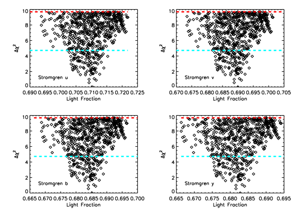
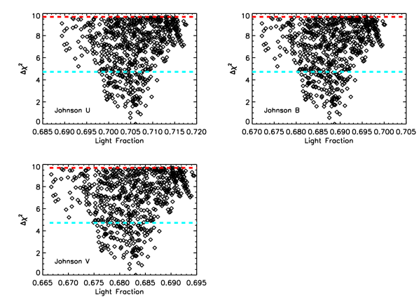
As mentioned by Torres et al. (2010) an important consistency check of our light curve solution is that the light fraction $l_{f,1}=\frac{l_{1}}{l_{1}+l_{2}}$ determined from spectroscopy and photometry agree. Given the small degeneracy between $R_{1}$ and $R_{2}$ as seen in Figure 8, we compare our photometrically determined light fraction with the light fraction from the HERMES spectral disentangling and a previous combined light curve and spectral disentangling analysis from Hensberge et al. (2000). We find that all three light fractions agree with each other to within 1.2$\sigma$. A comparison of light fractions is shown in Table 5.

For each of the $\approx 10^{5}$ light curve fits to our 40 yrs of photometry data, we compute the light fraction at each of the passbands Johnson $UBV$ and Strömgren $uvby$ photometry, $l_{f,1}(\lambda)=\frac{l_{1}(\lambda)}{l_{1}(\lambda)+l_{2}(\lambda)}$ where $l_{1}(\lambda)$ and $l_{2}(\lambda)$ are the contribution of the primary and secondary star to the total light at a specific passband out of eclipse. The distribution of light fractions $l_{f,1}$ for light curve models with confidence intervals of $1\sigma$ and $2\sigma$ are shown in Figures 9 and 10.

4.3 Comparison with Hensberge et al. (2000)

Hensberge et al. (2000) uses an iterative, combined light curve and spectral disentangling analysis using the Wilson-Devinney light curve modeling program to compute their light cure parameters. We find that $R_{1}=$$5.23\pm 0.06$ $\mbox{R}_{\mbox{$\odot$}}$ from Hensberge et al. (2000) is $2.5\sigma$ discrepant from our best fit $R_{1}=$$5.41\pm 0.04$ $\mbox{R}_{\mbox{$\odot$}}$. We find that our inclination $i=$$72.09\pm 0.06$ deg is 1.6$\sigma$ discrepant from $i=$$72.58\pm 0.30$ deg from Hensberge et al. (2000). These discrepancies are likely due to the addition of apsidal motion and an updated eccentricity determined in Garcia et al. (2011). Apsidal motion and eccentricity can affect the potentials $\Omega_{1}$ and $\Omega_{2}$ and hence the determination of the radii at a low level. The potential $\Omega$ for a non-circular orbit is a function of eccentricity (see Wilson, (1979)). The addition of more light curve epochs may also play a role. Hensberge et al. (2000) only uses the 1991-1994 light curve epoch with Strömgren $uvby$ photometry. As a check, we also recover the Hensberge et al. (2000) light curve solution when we fit only the 1991-1994 light curve epoch. Finally, simply the addition of more photometry data points may play a role. We use 3489 photometry data points in our light curve solution, whereas Hensberge et al. (2000) use 992. Our best fit secondary radius $R_{2}=$$4.29\pm 0.05$ $\mbox{R}_{\mbox{$\odot$}}$ is in agreement with $4.32\pm 0.07$ $\mbox{R}_{\mbox{$\odot$}}$ from Hensberge et al. (2000). Our best fit temperature ratio $\frac{T_{2}}{T_{1}}=$$0.858\pm 0.002$ is in agreement with the temperature ratio of $0.88\pm 0.020$ from an analysis of the disentangled component spectra (Hensberge et al. 2000).

5 Results: Absolute Dimensions and Apsidal Motion of V578 Mon

The absolute dimensions and other fundamental properties of V578 Mon are compiled in Table 11. Here we detail how each fundamental parameter for V578 Mon is compute in order of which they appear in Table 11:

1. Orbital Period. We adopt the orbital period $P=2.4084822$ d from Hensberge et al. (2000).

2. Masses. The component masses M${}_{1}=$$14.54\pm 0.08$ $\mbox{M}_{\mbox{$\odot$}}$ and M${}_{2}=$$10.29\pm 0.06$ $\mbox{M}_{\mbox{$\odot$}}$ are determined from the spectroscopic orbit analysis from Hensberge et al. (2000). We do not use RVs from our hermes spectroscopy because the caspec spectra have higher S/N - however, our analysis of the hermes spectroscopy reconfirm the spectroscopic orbit.

3. Radii. We find precise uncertainties of $<1.5$% for the primary radius $R_{1}=$$5.41\pm 0.04$ $\mbox{R}_{\mbox{$\odot$}}$ and secondary radius $R_{2}=$$4.29\pm 0.05$ $\mbox{R}_{\mbox{$\odot$}}$ from our confidence intervals in Figure 8.

4. Temperatures. We find a $0.3$% error on our temperature ratio $\frac{T_{2}}{T_{1}}=$$0.858\pm 0.002$ from our confidence intervals. Combined with the adopted temperature of the primary star T${}_{1}=$$30000\pm 500$ K (Hensberge et al. 2000), our temperature ratio of $\frac{T_{2}}{T_{1}}$ yields a secondary temperature of T${}_{2}=$$25750\pm 435$ K via propagation of errors.

5. Rotational Velocities. We compute surface rotational velocities of v${}_{\rm 1,rot}=$$123\pm 5$ km s^-1 and v${}_{\rm 2,rot}=$$99\pm 3$ km s^-1 using the observed projected surface velocities v${}_{1}\sin{i}=$$117\pm 4$ km s^-1 and v${}_{2}\sin{i}=$$94\pm 2$ km s^-1 from Hensberge et al. (2000) and our inclination of i$=$$72.09\pm 0.06$. The uncertainty on rotational velocities are computed from propagating the error on the inclination $i$ and the observed v$\sin{i}$.

6. Surface Gravities. We compute the surface gravity $\log{g}$ from our masses and radii, finding $\log{g_{1}}=$$4.133\pm 0.018$ cm s^-2 and $\log{g_{2}}=$$4.185\pm 0.021$ cm s^-2. We compute the uncertainty on $\log{g}$ via error propagation:

   $$\sigma_{\log{g}}=\sqrt{(\frac{\sigma_{M}}{M\ln{10}})^{2}+(\frac{2\sigma_{R}}{R\ln{10}})^{2}}$$ (5)

   Where $\sigma_{M}$ is the uncertainty on the mass and $\sigma_{R}$ is the uncertainty on the radius.

7. Luminosities. From our radii and temperatures, we compute compute luminosities for the primary and secondary star of $\log{\frac{L_{1}}{L_{\odot}}}=$$4.33\pm 0.03$  and $\log{\frac{L_{2}}{L_{\odot}}}=$$3.86\pm 0.03$. We compute the uncertainty on the luminosity using a similar error propagation as above, using errors from the temperature and radii, $\sigma_{T}$ and $\sigma_{R}$.

8. Synchronicity Parameters. We find the components of V578 Mon to be close but not exactly tidally locked, with $F_{1}=$$1.08\pm 0.04$ and $F_{2}=$$1.10\pm 0.03$. The synchronicity parameter $F=\frac{w}{w_{\rm orb}}$, where $w$ is the rotational velocity at the surface $v_{\rm rot}$ and $w_{\rm orb}=\frac{2\pi R}{P}$ is the synchronous velocity. We compute the uncertainty via propagation of error from $\sigma_{R}$, error on inclination $\sigma_{i}$, and error on projected rotational velocities $\sigma_{v\sin{i}}$.

9. Internal Structure Constant. One of us (Dr. Claret) computes the newtonian and general relativistic contributions to the observed internal structure constant, $\log{k_{\rm 2,newt}}=$$-1.975\pm 0.017$and $\log{k_{\rm 2,GR}}=$$-3.412\pm 0.018$.

6 The Stellar Evolution Models and Tests

We compare the absolute dimensions of V578 Mon to the stellar evolution models of three separate groups: (1) Geneva models of Georgy et al. (2013) and Ekström et al. (2012) hereafter Geneva13; (2) Utrecht models of Brott et al. (2011) here after Utrecht11 ; and (3) Granada models of Claret (2004, 2006) hereafter Granada04. We assume that both stars have the same initial chemical composition and age, as expected for tight binary systems. We perform two tests: (1) The “isochrone test” , which tests the ability of stellar evolution models to produce stars with different masses, radii, temperatures, rotational velocities, and surface compositions at the same age; and (2) The “apsidal motion test” which tests the ability of the stellar evolution models to reproduce the observed internal structure constant $\log{k_{2}}$ as determined from the observed apsidal motion.

A comparison of the basic input physics of the models is given in Table 12. The models use the same opacity tables of Iglesias & Rogers (1996). The mixing length $\alpha_{\rm MLT}\equiv\frac{l}{H_{p}}$ for all three sets of models differ by only $0.18$ at maximum. The stellar evolution models use similar mass loss treatment from the prescription by Vink et al. (2001). Given the probable young age of V578 Mon due to its location in the open cluster NGC 2244 of the Rosette Nebula, the components of V578 Mon are not expected to have undergone significant mass loss (Vink et al. 2001).

However, all three sets of models differ on the choice of the convective core overshoot parameter $\alpha_{\rm ov}$. For the H and He burning phases of the convective core, the convective core size of the star is enlarged by $R_{\rm cc}=R_{cc}(1+\frac{d_{\rm over}}{H_{p}})$, where $\alpha_{\rm ov}\equiv\frac{d_{\rm over}}{H_{p}}$ in units of pressure scale height. The overshoot parameter is designed to accomodate for the non zero velocity of the material moving from the convective core to radiative zone of the star. Observationally, a larger overshoot parameter means longer MS lifetimes for a given star, and thus older ages. The Geneva13 models use a small convective core overshoot of $\alpha_{\rm ov}=0.1$ calibrated on width of the main sequence for stars with masses $M=1.35-9.0~{}\mbox{M}_{\mbox{$\odot$}}$ which is characterized by the red most point on the B-V, $M_{V}$ HR diagram (see figure 8 of Ekström et al. (2012)). The width of the main sequence is defined theoretically by the end of the hydrogen burning phase. The Utrecht11 models use a high convective core overshoot of $\alpha_{\rm ov}=0.335$ which is calibrated using the observed width of the main sequence from the VLT-FLAMES survey of B stars (Evans et al. 2005; Hunter et al. 2007). The convective core overshoot parameter $\alpha_{\rm ov}=0.335$ is chosen such that a 16 $\mbox{M}_{\mbox{$\odot$}}$ star ends its MS lifetime when $\log{g}=3.2$. This $\log{g}$ coincides with the drop in B star rotation rates in a $\log{g}$-$v\sin{i}$ diagram, which is interpreted as an estimate of the width of the main sequence for B stars. See Brott et al. (2011) for an in depth discussion. The Granada04 models utilize a moderate convective core overshoot $\alpha_{\rm ov}=0.2$, though we performed several tests varying $\alpha_{\rm ov}$.

Rotationally driven mixing can bring more H and He from the envelope to the core, thus extending the MS lifetime of the star - likewise a larger overshoot parameter extends the size of the core, leading to a longer MS lifetime. The Granada04 models do not incorporate rotational mixing, while the Geneva13 and Utrecht11 models do. However - All three sets of models include rotation. All three sets of models use similar metallicity compositions of near solar. The initial bulk composition for V578 Mon is expected to be close to solar given that Mg surface abundance is within error of the solar surface abundance, despite the fact that several atmospheric abundances such as C, N and O are somewhat metal poor compared to the Sun (Pavlovski & Hensberge 2005). This is because Mg abundance is not expected to be altered from the initial abundance in a star, where as C, N and O atmospheric abundances could vary in V578 Mon due to rotational mixing (Lyubimkov et al. 2005). However, given that the C, N and O atmospheric abundances of V578 Mon may be lower than solar, the metallicity of V578 Mon still remains as a source of systematic error in comparing the evolution models to the observations.

The Granada04 models also compute the internal structure constants $\log{k_{2}},\log{k_{3}}$ and $\log{k_{4}}$ allowing for a test of the internal structure of V578 Mon via apsidal motion. Here we consider only the $k_{2}$ constant, given that $k_{3}$ and $k_{4}$ are very small. For V578 Mon, the tidal Love numbers quantify the deformation for each star’s gravity field due to the companion.

6.1 Isochrone Test for V578 Mon

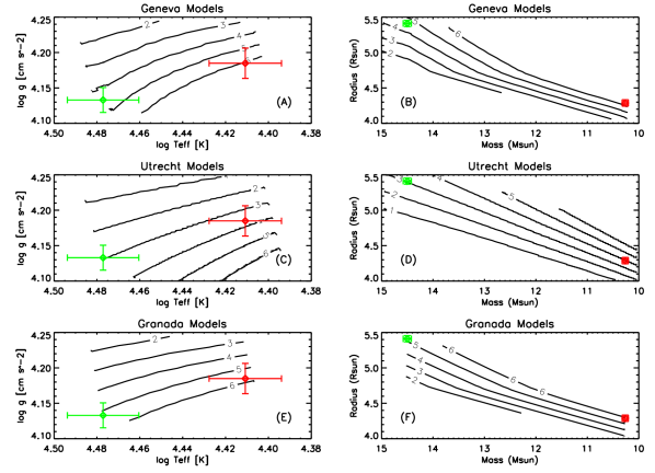
In Figure 11, we place the primary and secondary star on mass-radius and $\log{g}-\log{T_{\rm eff}}$ isochrones for each set of models. For the stellar evolution models to pass the “isochrone test” the models should predict a common age for both components of V578 Mon within uncertainty. Given how different the masses of the primary and secondary star for V578 Mon are the “isochrone test” provides a stringent test of stellar evolution models. We also match all evolution models to the rotational velocities of the primary and secondary star.

We find several Geneva13, Utrecht11 and Granada04 models predict masses, radii and temperatures for the components of V578 Mon that fall within $1\sigma$ uncertainty of the measured absolute dimensions. Therefore we estimate an age range for each star as shown in Table 12. The age difference for Geneva13, Utrecht11 and Granada04 models is given as the smallest possible difference between the ages of the two stars given age range of each star.

For the Geneva models we use isochrones with initial rotational velocities $\frac{v_{i}}{v_{\rm crit}}=0.30$ and $\frac{v_{i}}{v_{\rm crit}}=0.35$ which allows us to match the observed rotational velocities for each star. We interpolate the model evolution tracks for the primary and secondary star using the online interactive tool provided by the Geneva group . Attempts to match the observed rotational velocities of V578 Mon with lower ($\frac{v_{i}}{v_{\rm crit}}<0.30$) or higher ($\frac{v_{i}}{v_{\rm crit}}>0.40$) initial velocities for either star were unsuccessful. Attempts to find a single initial rotational velocity to reproduce the current observed rotational velocities for both stars with reasonable predicted radii and masses were also unsuccessful. However, given that V578 Mon is very near synchronization with the orbital period ($F_{1}=$$1.08\pm 0.04$, $F_{2}=$$1.10\pm 0.03$), the rotational history of V578 Mon could be different from the best matched $\frac{v_{i}}{v_{\rm crit}}$ found here. If the initial velocities of the components of V578 Mon were larger at the ZAMS than the orbital velocity, the stars could spin down to synchronize with the orbital velocity. Conversely, if $\frac{v_{i}}{v_{\rm crit}}$ was smaller than the orbital velocities, then the components of V578 Mon could spin up (Song et al. 2013). From Table 13 we find an age difference of 1.6 Myr for mass-radius isochrones, and an age difference of only $0.1$ Myr for $\log{g}-\log{T_{\rm eff}}$ isochrone. It is easier to find consistency for the latter isochrones given our uncertainty in the effective temperatures of the two stars. We find that a primary radius of $R_{1}=5.50~{}\mbox{R}_{\mbox{$\odot$}}$ and a secondary star radius of $R_{2}=5.20~{}\mbox{R}_{\mbox{$\odot$}}$ yields common ages for the Geneva13 models. However, these radii are $3\sigma$ larger and $3\sigma$ smaller than our best fit model, respectively.

For the Utrecht11 models we use isochrones that match the observed surface velocities of the components of V578 Mon, v${}_{\rm 1,rot}=$$123\pm 5$ km s^-1 and $v_{\rm 2,rot}=$$99\pm 3$ km s^-1. The Utrecht11 models are computed at very small steps of mass and initial rotational velocity, such that interpolating between model tracks is unnecessary. From Table 13 we a marginally common age (age difference $0.4$ Myr) for mass-radius isochrones, and a common age of $3.5\pm 1.5$ Myr for $\log{g}-\log{T_{\rm eff}}$ isochrone. The models were computed at solar metallicity by Dr. Brott (private comm.).

We compute the Granada04 models at the masses of primary and secondary star and chose rotational velocities to match the observed rotational velocities of V578 Mon. We attempt to match the absolute dimensions of V578 Mon to $\log{g}-\log{T_{\rm eff}}$ or alternatively mass-radius isochrones for V578 Mon. We find an age gap of 1.5 Myr for mass-radius isochrones, and a marginally common age for $\log{g}-\log{T_{\rm eff}}$ isochrones, when both stars have an overshoot of $\alpha_{\rm ov}=0.2$. Again - finding a match on the $\log{g}-\log{T_{\rm eff}}$ isochrones is easier given the greater uncertainty in the effective temperatures.

In an attempt to match the ages of the two stars on a mass-radius isochrone, we also compute Granada04 models for $\alpha_{\rm ov}=0.4$ and $\alpha_{\rm ov}=0.6$. Figure 12 demonstrates the time evolution of the radii for V578 Mon for these different models. We find a near match on a single mass-radius isochrone with an age difference of only 0.2 Myr - if we assume that the primary star has a convective overshoot $\alpha_{\rm ov}=0.6$ and the secondary star has a convective overshoot of $\alpha_{\rm ov}=0.2$. We also find a common age of $5.5\pm 1.0$ Myr for the $\log{g}-\log{T_{\rm eff}}$ isochrone. This does not mean that an $\alpha_{\rm ov}=0.6$ for the primary star is correct for V578 Mon - merely that a higher convective overshoot allows for compatible ages between the two stars. High convective overshoot has been found to work in matching other EBs on a single isochrone (Claret 2007).

In general, we find younger ages by $\approx 1$ Myr for the Utrecht11 models of V578 Mon and similar ages for the Geneva13 and Granada04 models. This can be attributed to the larger convective overshoot of $\alpha_{\rm ov}=0.355$ included in Utrecht11 models than in Geneva13 models ($\alpha_{\rm ov}=0.2$). While the primary star for the Granada04 models does have an even higher convective overshoot of $\alpha_{\rm ov}=0.6$, the models do not include rotational mixing, which also extends the main sequence lifetime of the stars.

6.2 Apsidal Motion Test for V578 Mon

Measurement of apsidal motion in eccentric binary systems allow for a stringent test of the internal structure constant $k_{\rm 2,theo}$ predicted from stellar evolution models (e.g. Claret & Giménez 2010). It is not possible to separate out each individual star’s contribution to the apsidal period U from newtonian apsidal motion.

The apsidal motion for V578 Mon was measured by Garcia et al. (2011). The observed apsidal motion of the V578 Mon, $\dot{\omega}_{\rm tot}=0.07089^{+0.00021}_{-0.00013}$ deg cycle^-1, has contributions from both newtonian and general relativity components (Claret & Giménez 2010):

$$\dot{\omega}_{\rm obs}=\dot{\omega}_{\rm newt}+\dot{\omega}_{\rm GR}$$ (6)

where $\dot{\omega}_{\rm GR}$ is given by

$$\dot{\omega}_{\rm GR}=0.002286\frac{M_{1}+M_{2}}{a(1-e^{2})}$$ (7)

We find that $\dot{\omega}_{\rm GR}=$$0.002589\pm 0.000015$ which is only $4\%$ of the newtonian apsidal motion $\dot{\omega}_{\rm newt}=$$0.06830\pm 0.00017$.

Both the newtonian and general relativistic observed apsidal motions $\dot{\omega}_{\rm newt}$ and $\dot{\omega}_{\rm GR}$ have associated observed internal structure constants $k_{\rm 2,obs}$. The internal structure constant is twice the tidal love number (Kramm et al. 2011), and is related to the density profiles, degree of sphericity, orbital parameters, masses, and rotation rate of both components of a binary star. Specifically, the internal structure constant is related to the solution of the Radau differential equation as in equation 3 of Claret & Giménez (2010). Importantly - constant $k_{\rm 2,obs}$ is one the few ways to directly constrain the internal structure of stars.

From the precise observed apsidal motion, we compute the observed internal structure constant, $k_{\rm 2,obs}$ = $k_{\rm 2,obs}(M_{1},M_{2},R_{1},R_{2},P,U,F_{1},F_{2},e)$, where U is the apsidal period, given by the equations (adopted from Claret & Giménez (2010)):

$$k_{\rm 2,obs}=\frac{1}{c_{21}+c_{22}}\frac{P}{U}$$ (8)

$$c_{2i}=[(F_{i})^{2}(1+\frac{M_{3-i}}{M_{i}})f(e)+15\frac{M_{3-i}}{M_{i}}g(e)](\frac{R_{i}}{a})^{5}$$ (9)

$$f(e)=(1-e^{2})^{-2}$$ (10)

$$g(e)=\frac{(8+12e^{2}+e^{4})f(e)^{2.5}}{8}$$ (11)

We compute the internal structure constant due to the newtonian apsidal motion, $\log{k_{\rm 2,newt}}=$$-1.975\pm 0.017$, and due to general relativity, $\log{k_{\rm 2,GR}}=$$-3.412\pm 0.018$. The newtonian apsidal motion is much larger than the general relativistic component, and therefore the internal structure constant is also much larger.

We compute the theoretical internal structure constant, $k_{\rm 2,theo}$ using the methods of Claret & Giménez (2010). The theoretical $k_{2}$ constant was corrected for by rotation (Claret 1999) and dynamical tides (Willems & Claret 2002). The theoretical internal structure constant is a combination of the internal structure constants for both star, such that

$$k_{\rm 2,theo}=\frac{c_{21}k_{21}+c_{22}k_{22}}{c_{21}+c_{22}}$$ (12)

which can then be compared to observations.

We find the predicted newtonian apsidal motion to be $\dot{\omega}_{\rm theo}=$$0.06883\pm 0.00017$ and consequently the predicted newtonian internal structure constant to be $\log{k_{\rm 2,theo}}=$$-2.005\pm 0.025$. This is in very good agreement with the observed $\log{k_{\rm 2,obs}}=$$-1.975\pm 0.017$. From equation 9, the parameter $c_{12}$ is about 67% larger than $c_{22}$. Therefore, the weighted contribution of the primary dominates the theoretical apsidal motion. V578 Mon is a relatively young system - therefore, $\log{k_{\rm 2,theo}}$ is almost constant during the early phases of stellar evolution. The “apsidal motion test” is therefore complementary to the “isochrone test”. Claret & Giménez (2010) compile a list of eclipsing binaries with apsidal motion, demonstrating good agreement between observed and predicted apsidal motions. V578 Mon continues this trend of agreement between theoretical and observational internal structure constants. For this relatively young system, matching the radii, temperatures and masses isochrones is key, given that we have so few young massive EBs with non-equal mass ratio.

7 Conclusion

We have determined the absolute dimensions of the massive, detached eclipsing binary V578 Mon, which is a member of young star forming region NGC 2244 in the Rosette Nebula. We confirm that the the previously published spectroscopic orbit of Hensberge et al. (2000) agree with our current spectroscopic orbit of V578 Mon. From our hermes spectra, we find that our photometric light ratio from the light curve analysis is fully compatible with the disentangled component spectra of V578 Mon.

From 40 yr of Johnson UBV and Strömgren $uvby$ photometry we determine updated radii, measure the temperature ratio and light ratio for the components of V578 Mon. We determine the radii to better than $1.5\%$ accuracy, and carefully map out parameter space in order to reveal any possible degeneracies. We also compare our global best fit light curve model with models that include different limb darkening parameters, a different assumed temperature for the primary star, light reflection or third light finding little effect on our global model. We do not unambiguously rule out light reflection or a third body, but we confirm that these additional complications to the light curve model will not affect our final solution.

We have compared our observed masses, radii, temperatures and rotational velocities to stellar evolution models of the Geneva, Utrecht, and Granada groups. We find no common match in predicted ages for mass-radius isochrones of the Geneva13 models. We find an age difference of only $0.1$ Myr in predicted ages for the Geneva13 models for $\log{g}-\log{T_{\rm eff}}$ isochrones. For the Utrecht11 models, we find a marginally common predicted age with an age difference of only 0.4 Myr for the mass-radius isochrones. For the $\log{g}-\log{T_{\rm eff}}$ isochrones we find common ages of $3.5\pm 1.5$ Myr for the Utrecht11 models. For the Granada04 models, we find a small age gap of only 0.2 for the mass-radius isochrone, when the primary star has a quite large convective overshoot of $\alpha_{\rm ov}=0.6$. We do not find common ages for the mass-radius isochrone for the Granada04 models when the convective overshoot for both stars is a more moderate $\alpha_{\rm ov}=0.2$.

This work suggests that models with larger convective overshoot predict a closer common age for the components of V578 Mon than models with a more conventional overshoot of $\alpha_{\rm ov}=0.2$ pressure scale heights. Evolutionary models with larger convective overshoot extends the size of the convective core for massive stars, thus extending the main sequence lifetime and allowing for isochrones to predict a common age for V578 Mon. However - rotational mixing also can prolong the main sequence lifetime, making the two effects some what degenerate. The radii may in a small way be dependent upon effective temperatures, which are based on imperfect atmosphere models. Furthermore, there are small systematic residuals of $0.005$ mag in the light curve fits which may in a small way affect the radii. Finally, effects of binarity, while likely small, are not taken into account: the side of each star facing the other may be heated and the addition to the potential $\Omega$ from the companion is not taken into account into the models. The binarity of V578 Mon may cause single star models explored here to not be applicable.

Given the short apsidal period of V578 Mon of $33.48^{+0.10}_{-0.06}$ years, our photometry cover one full apsidal motion period. Combined with our precise measurement of the radii of V578 Mon we compute the internal structure constant $\log{k_{2}}$ finding that our observed $\log{k_{\rm 2,obs}}=$$-1.975\pm 0.017$  in agreement with the theoretical internal structure constant $\log{k_{\rm 2,theo}}=$$-2.005\pm 0.025$.

V578 Mon is a particularly important system for testing stellar evolution models given young age and the difference of $\approx 30\%$ in the masses of the primary and secondary component star. B-type detached eclipsing binaries such as V1388 Ori and V1034 Sco have similar differences in mass of 40% and 50% respectively, meaning these systems are also of particular importance to providing constraints on stellar evolution models. However, V578 Mon is unique among such systems by virtue of its young age, thus providing the strongest constraints on the models at the earliest stages of massive stellar evolution.

Future work may include comparing the carefully vetted sample of high mass EBs in the Torres et al. (2010) sample to evolutionary models, include more recent massive EBs such as V 380 Cyg (Tkachenko et al. 2014) and LMC 172231 and ST2-28 (Massey et al. 2012), to see if larger convective overshoot parameters allow for common predictions of age.

Figure 1: Massive ($>10\mbox{M}_{\mbox{$\odot$}}$) detached eclipsing binaries with accurate masses and radii better than $2\%$ are scarce. There are only 9 such systems (black triangles) including V578 Mon (green circles). This list of eclipsing binaries is adapted from Torres et al. (2010). The error bars on the mass and radii are smaller than the plotted symbols. Of these eclipsing binaries, V578 Mon is simultaneously one of the youngest and lowest mass ratios $q=\frac{M_{2}}{M_{1}}$.

Figure 2: Fits (red) to the hermes spectra (blue) obtained during the primary and secondary eclipse of V578 Mon. The disentangled component spectra obtained from time-series of observed spectra out-of-eclipse are shown above in black. The light ratio from the light curve analysis agrees to within uncertainty the light ratio derived from the in eclipse spectra. The light contribution of each component in the phases of the eclipses were calculated from the final light curve solution.

(a) He 4388

(b) He 4471

(c) He 4541

(d) He 4686

Figure 3: Optimal fitting for the four helium lines, He I 4388 Å, He I 4471 Å, He II 4541 Å, and He II 4686 Å for the out-of-eclipse HERMES spectra. In each panel helium line profiles for both components are shown (blue solid line). Optimal fitting was performed on all 4 lines simultaneously (red solid line). These are reconstructed helium profiles from disentangled spectra using the light ratio and surface gravities fixed to the final solution. A color version of this figure is available in the online journal.

Figure 4: Representative fits to light curves from 2005–2006, 1999–2000, 1995–1996 and 1994–1995 in the Johnson $B$ passband from global fits to all light curve data, offset for clarity. The residuals to the fits $(O-C)$ are shown above.

Figure 5: Same as Fig. 4, but showing Johnson $V$ band light curves and fits.

Figure 6: Same as Fig. 4, but showing Strömgren $uvby$ light curves and fits.

Figure 7: Same as Fig. 4, but showing 1973–1977 Johnson $UBV$ light curves and fits.

Figure 8: Degeneracies for our best fit light curve solution. The blue squares, red triangles and black diamonds correspond to difference in chi square from the global best fit solution $\Delta\chi^{2}=4.72$,$9.70$, and $16.3$ respectively. For four parameters of interest these $\Delta\chi^{2}$ correspond to $1\sigma$, $2\sigma$ and $3\sigma$ respectively. There is a small degeneracy between the sum of the radii $R_{1}+R_{2}$ and $i$. This degeneracy is typical for detached eclipsing binaries with circular or near circular orbits. Similarly, there is a small degeneracy between the primary and secondary radii $R_{1}$ and $R_{2}$. The global best fit solution is marked with an X. There is no degeneracy between the temperature ratio $\frac{T_{2}}{T_{1}}$ and inclination $i$ or sum of the radii $R_{1}+R_{2}$. A color version of this figure is available in the online journal.

Figure 9: The light fractions $l_{f,1}=\frac{l_{1}(\lambda)}{l_{1}(\lambda)+l_{2}(\lambda)}$ for light curve fits within $1\sigma$ (below the blue line) and $2\sigma$ (below the red line) uncertainty for the Stromgren $uvby$ photometry. Our light fractions are consistent with the light fractions computed from Hensberge et al. (2000). A color version of this figure is available in the online journal.

Figure 10: Same as Figure 9 except for the Johnson UBV photometry.

Figure 11: The best matches to observations are the Utrecht11 and Granada04 models, which both use larger than conventional overshoot of $\alpha_{\rm ov}=0.2$ - see Table 13 for details. Isochrones are in steps of 1 Myr of the Geneva13, Utrecht11 and Granada04 models. The green point is the primary star, and the red point is the secondary star. All models have rotational velocities that match the observed velocities of V578 Mon $v_{\rm 1,rot}=$$123\pm 5$ km s^-1 and $v_{\rm 2,rot}=$$99\pm 3$ km s^-1. A color version of this figure is available in the online journal.

Figure 12: The time evolution of the radii for V578 Mon from Granada04 models computed for the masses of the V578 Mon primary and secondary. Dot-dashed, dashed, and solid lines are evolutionary models at convective overshoot of $\alpha_{\rm ov}$ of $0.2$, $0.4$ and $0.6$ pressure scale heights respectively. Horizontal lines are the upper and lower limit of uncertainty on the primary star and secondary star radius respectively. The models predict a common age of 5.5 Myr - if we use a high convective overshoot of $\alpha_{\rm ov}=0.6$ evolution model for the primary star and $\alpha_{\rm ov}=0.2$ for the secondary star.

Table 1: Identifications, location and combined photometric parameters for eclipsing binary V578 Mon

	V578 Mon	Reference
Henry Draper number	HD 259135	Cannon & Pickering (1923)
Bonner Durchmusterung	BD +04°1299	Argelander (1903)
Hoag number	NGC 2244 200	Hog et al. (1998)
$\alpha_{2000}$	06 32 00.6098	Hog et al. (1998)
$\delta_{2000}$	+ 04 52 40.902	Hog et al. (1998)
Spectral type	B0V + B1V	Hensberge et al. (2000)
$V$	8.542	Ogura & Ishida (1981)
$V-I$	0.262	Wang et al. (2008)
$B-V$	+ 0.165	Ogura & Ishida (1981)
$U-B$	$-$ 0.727	Wolff et al. (2007)
$V-R$	+ 0.452	Wang et al. (2008)

Table 2: V578 Mon Light Curves

Observatory	Year	Filter	$\sigma_{0}$	$\sigma$	N
			[mag]	[mag]
1 KPNO	1967-84	Johnson $U$	0.004	$0.016$	251
		Johnson $B$	0.004	$0.012$	256
		Johnson $V$	0.004	$0.013$	217
2SAT	1991–94	Strömgren $u$	0.0029	0.0067	248
		Strömgren $b$	0.0023	0.0046	248
		Strömgren $v$	0.0023	0.0054	248
		Strömgren $y$	0.0030	0.0053	248
3APT	1994–95	Johnson $V$	0.0037	$0.0022$	260
		Johnson $B$	0.001	$0.0040$	254
APT	1995–96	Johnson $V$	0.002	$0.0035$	95
		Johnson $B$	0.001	$0.0037$	96
APT	1999–2000	Johnson $V$	0.002	$0.0058$	259
		Johnson $B$	0.001	$0.0078$	246
APT	2005–06	Johnson $V$	0.002	$0.0036$	284
		Johnson $B$	0.001	$0.0044$	283

Note. — ¹16-inch telescope at Kitt Peak (KPNO)

²0.5 m telescope at La Silla (SAT)

³TSU-Vanderbilt 16-inch telescope at Fairborn University (APT)

Table 3: Hermes Observations

Phase	BJD-2450000.000	Exp Time [s]
0.9957	5904.586	2100
0.0060	5904.611	2100
0.0168	5904.637	2100
0.0272	5904.662	2100
0.0376	5904.687	1980
0.0476	5904.711	1980
0.0613	5909.561	1500
0.0692	5909.580	1500
0.1128	5914.502	2100
0.1231	5914.527	2100
0.1530	5914.599	2100
0.1634	5914.624	2100
0.2259	5907.549	2100
0.2363	5907.574	2100
0.2803	5912.497	2100
0.2907	5912.522	2100
0.3434	5912.649	2100
0.3534	5912.673	2100
0.4432	5905.664	2100
0.4449	5910.485	2300
0.4536	5905.689	2100
0.4565	5910.513	2300
0.4673	5910.539	2100
0.4777	5910.564	2100
0.5010	5910.620	2100
0.5113	5910.645	2100
0.6427	5908.553	2200
0.6535	5908.579	2200
0.7187	5913.553	2100
0.7291	5913.578	2100
0.7945	5906.510	2100
0.8049	5906.535	2100
0.9278	5911.648	2200
0.9390	5911.675	2200

Note. — Time-series Hermes spectroscopy of V578 Mon. Each exposure is less than 0.01 of the orbital period for V578 Mon of $2.4084822$ days. The time series spectra were obtained to cover the out-of-eclipse, primary eclipse and secondary eclipse phases.

Table 4: Radial Velocity Solutions

	$q$	$K_{1}$	$K_{2}$	$e$
		[km s-1]	[km s-1]
Hensberge et al. (2000) (LC+Spectroscopy)	0.7078$\pm 0.0002$	259.8	183.9	0.0867
Hensberge et al. (2000) RV only	0.705$\pm$0.004	259.8$\pm$0.8	184.4	0.0836$\pm 0.0008$
HERMES Spectra, $e$ fixed	0.710	259.8	184.5	0.07755
HERMES Spectra, $e$ and $\omega$ fixed	0.709	259.4	184.0	0.07755

Table 5: Light Fraction Comparison

Method	Wavelength $\lambda$	Light Fraction $\frac{l_{1}}{l_{1}+l_{2}}$
	[nm]
Light Curve Analysis (this work)	Johnson U, 365	$0.706\pm 0.008$
	Johnson B, 445	$0.689\pm 0.007$
	Johnson V, 551	$0.683\pm 0.007$
	Stromgren u, 365	$0.710\pm 0.007$
	Stromgren v, 411	$0.690\pm 0.008$
	Stromgren b, 467	$0.685\pm 0.007$
	Stromgren y, 547	$0.683\pm 0.007$
Hensberge et al. (2000)	Stromgren v, 411	$0.675\pm 0.006$
	Stromgren b, 467	$0.683\pm 0.006$
	Stromgren y, 547	$0.692\pm 0.006$
HERMES Spectroscopy	400-500	$0.700\pm 0.02$

Table 6: Light Curve Parameter Ranges Explored

Parameter	Max	Min	Coarse Grid Spacing	Fine Grid Spacing
Primary Surface Potential, $\Omega_{1}$	5.36	4.80	$0.045$	$0.005$
Secondary Surface Potential, $\Omega_{2}$	5.26	4.40	$0.045$	$0.005$
Inclination, $i$ [deg]	73.15	70.00	$0.2$	$0.0005$
Temperature Ratio, $\frac{T_{2}}{T_{1}}$	0.875	0.843	$0.0012$	$0.03$

Table 7: Light Curve Analysis Results and Comparison

Light Curve Parameters	This Work & Garcia et al. (2011)	H2000
Primary Surface Potential, $\Omega_{1}$	$4.88\pm 0.03$	$5.02\pm 0.05$
Secondary Surface Potential, $\Omega_{2}$	$4.89\pm 0.04$	$4.87\pm 0.06$
Temperature Ratio, $\frac{T_{2}}{T_{1}}$	$0.858\pm 0.002$	$0.88\pm 0.02$
Inclination, $i$ [deg]	$72.09\pm 0.06$	$72.58\pm 0.3$
Eccentricity, $e$	$0.07755^{+0.00018}_{-0.00026}$	$0.0867\pm 0.0006$
Angle of Periastron, $w$ [deg]	$159.8\pm 0.33$	$153.3\pm 0.6$
Ephemeris, HJD0 [d]	$2449360.6250$	$2449360.6250$
Total Apsidal Motion, $\dot{\omega}_{\rm tot}$ [deg cycle-1]	$0.07089^{+0.00021}_{-0.00013}$
Light Curve Filters	Strömgren $uvby$, Johnson $UBV$	Strömgren $uvby$
Total Light Curve Points	$3489$	$992$

Note. — The uncertainties on light curve parameters $\Omega_{1}$, $\Omega_{2}$, $i$ and $\frac{T_{2}}{T_{1}}$ are determined from confidence intervals in Figure 8. Light curve parameters $e$, $w$ and $\dot{\omega}_{\rm tot}$ are taken from Garcia et al. (2011). This work utilizes photometry that span one full apsidal motion period (U$=$$33.48^{+0.10}_{-0.06}$yr). In contrast to the Hensberge et al. (2000) analysis, this work incorporates apsidal motion in the light curve model. Finally, the temperature ratio from Hensberge et al. (2000) is measured from spectral disentangling.

Table 8: Limb Darkening Coefficients

Filter	$x_{1}$	$x_{2}$	$y_{1}$	$y_{2}$
Square Root Law (adopted)
Strömgren $u$	-0.096	-0.073	0.631	0.606
Strömgren $b$	-0.132	-0.115	0.672	0.659
Strömgren $v$	-0.129	-0.106	0.607	0.581
Strömgren $y$	-0.073	-0.044	0.612	0.581
Johnson $U$	-0.131	-0.115	0.685	0.675
Johnson $B$	-0.131	-0.110	0.654	0.638
Johnson $V$	-0.126	-0.105	0.602	0.578
Linear Law
Strömgren $u$	0.282	0.291	0.000	0.000
Strömgren $b$	0.272	0.281	0.000	0.000
Strömgren $v$	0.235	0.243	0.000	0.000
Strömgren $y$	0.293	0.304	0.000	0.000
Johnson $U$	0.280	0.291	0.000	0.000
Johnson $B$	0.262	0.273	0.000	0.000
Johnson $V$	0.235	0.242	0.000	0.000
Logarithmic Law
Strömgren $u$	0.450	0.452	0.252	0.242
Strömgren $b$	0.450	0.457	0.268	0.264
Strömgren $v$	0.397	0.398	0.242	0.233
Strömgren $y$	0.456	0.459	0.244	0.232
Johnson $U$	0.462	0.471	0.274	0.270
Johnson $B$	0.436	0.444	0.261	0.256
Johnson $V$	0.395	0.396	0.241	0.231

Note. — Our best fit model uses the square root limb darkening law. Fits with the linear cosine or logarithmic limb darkening law had little effect on our final light curve solution.

Table 9: A comparison of light curve models

Model	$\Omega_{1}$	$\Omega_{2}$	$i$	$\frac{T_{2}}{T_{1}}$	$\chi^{2}$
			[deg]
Best Fit	$4.88\pm 0.03$	$4.89\pm 0.04$	$72.09\pm 0.06$	$0.858\pm 0.002$	$3489.00$
Fitting for LD coefficients	$4.92$	$4.89$	$72.18$	$0.835$	$3299.11$
Linear Law	$4.92$	$4.89$	$72.15$	$0.860$	$3480.01$
Logarithmic Law	$4.91$	$4.88$	$72.14$	$0.858$	$3503.96$
Fix $T_{1}=28500$	$4.94$	$4.87$	$72.17$	$0.857$	$3460.16$
Fix $T_{1}=31500$	$4.92$	$4.89$	$72.15$	$0.867$	$3488.01$
Light Reflection	$4.90$	$4.92$	$72.20$	$0.856$	$3522.57$
Third Light	$4.94$	$4.87$	$72.24$	$0.855$	$3414.93$

Note. — The best fit model uses the square root limb darkening law, a fixed $T_{1}=$30000 K, no light reflection, and no third light.

Table 10: Third Light

Observatory	Year	Filter	$\frac{L_{3}}{L_{\rm tot}}$
APT	2005–06	Johnson $B$	0.0441
		Johnson $V$	0.0218
APT	1999–2000	Johnson $B$	0.0158
		Johnson $V$	0.0080
APT	1995–96	Johnson $B$	-0.0037
		Johnson $V$	0.0104
APT	1994–95	Johnson $B$	0.0059
		Johnson $V$	0.0046
SAT	1991–94	Strömgren $u$	-0.0116
		Strömgren $v$	-0.0004
		Strömgren $b$	0.0013
		Strömgren $y$	-0.0045
KPNO	1967-84	Johnson $U$	0.0163
		Johnson $B$	0.0467
		Johnson $V$	-0.0100

Note. — Our best fit light curve model includes no third light. The small amount of third light varies as a function of epoch.

Table 11: V578 Mon Absolute Dimensions

Parameter	Primary	Secondary
Orbital Period, P [d]	$2.4084822$
Mass, $M$ [$M_{\odot}$]	$14.54\pm 0.08$	$10.29\pm 0.06$
Radius, $R$ [$R_{\odot}$]	$5.41\pm 0.04$	$4.29\pm 0.05$
Effective Temperature, $T_{\rm eff}$ [K]	$30000\pm 500$	$25750\pm 435$
Surface Gravity, $\log{g}$ [cm s-2]	$4.133\pm 0.018$	$4.185\pm 0.021$
Surface Velocity, $v_{\rm rot}$ [km s-1]	$123\pm 5$	$99\pm 3$
Luminosity, $\log{\frac{L}{L_{\odot}}}$	$4.33\pm 0.03$	$3.86\pm 0.03$
Synchronicity Parameter, $F=\frac{w}{w_{orb}}$	$1.08\pm 0.04$	$1.10\pm 0.03$
Apsidal Period, U [yr]	$33.48^{+0.10}_{-0.06}$
Observed Newtonian Internal Structure Constant, $\log{k_{\rm 2,newt}}$	$-1.975\pm 0.017$

Table 12: Stellar Evolution Models Comparison

Physical Input	Geneva13	Utrecht11	Granada04
Composition [Z,Y,X]	[0.014,0.266,0.720]	[0.0122,0.2486,0.7392]	[0.014,0.271,0.715]
Overshoot, $\alpha_{\rm ov}$	0.10	0.355	0.6 pri, 0.2 sec
Mixing Length, $\alpha_{\rm MLT}$	1.60	1.5	1.68
Rotation	Yes	Yes	Yes
Rotational Mixing	Yes	Yes	No
Opacities	Iglesias & Rogers (1996)	Iglesias & Rogers (1996)	Iglesias & Rogers (1996)
Mass loss	Vink et al. (2001)	Vink et al. (2001)	Vink et al. (2001)

Table 13: Ages from Stellar Evolution Models

Model	Primary Age	Secondary Age	Age Diff (lower limit)	$\alpha_{\rm ov}$
	[Myr]	[Myr]	[Myr]	[Scale height]
Mass$-$Radius$-v_{\rm rot}$ Isochrones
Geneva13	4.3$-$4.6	6.2$-$7.1	1.6	0.1
Utrecht11	3.0$-$3.2	3.6$-$4.4	0.4	0.355
Granada04	5.0$-$5.3	5.5$-$6.3	0.2	0.6 pri, 0.2 sec
$\log{g}$-$\log{T_{\rm eff}}$-$v_{\rm rot}$ Isochrones
Geneva13	3.9$-$5.1	5.2$-$7.5	0.1	0.1
Utrecht11	2.6$-$3.8	2.4$-$5.2	Common age $3.5\pm 1.5$	0.355
Granada04	4.7$-$5.5	4.9$-$6.8	Common age $5.5\pm 1.0$	0.6 pri, 0.2 sec

Note. — The ages for the primary and secondary star are computed from evolutionary tracks at the masses of either star and solar metallicity. The Granada04 models were computed for a high convective overshoot of $\alpha_{\rm ov}=0.6$ pressure scale heights for the primary star, which allowed the models to match the observations. It easier to find a common age for the $\log{g}-\log{T_{\rm eff}}$ isochrone given the larger uncertainty on the effective temperatures of the stars.

References

- Argelander (1903) Argelander, F. W. A. 1903, Eds Marcus and Weber’s Verlag, Bonn (1903), 0
- Asplund et al. (2009) Asplund, M., Grevesse, N., Sauval, A. J., & Scott, P. 2009, ARA&A, 47, 481
- Avni (1976) Avni, Y. 1976, ApJ, 210, 642
- Bell et al. (1986) Bell, S. A., Hilditch, R. W., & Adamson, A. J. 1986, MNRAS, 223, 513
- Bouzid et al. (2005) Bouzid, M. Y., Sterken, C., & Pribulla, T. 2005, A&A, 437, 769
- Butler & Giddings (1985) Butler, K., & Giddings, J. R. 1985, Newsletter of Analysis of Astronomical Spectra, No. 9
- Brott et al. (2011) Brott, I., de Mink, S. E., Cantiello, M., et al. 2011, A&A, 530, A115
- Cannon & Pickering (1923) Cannon, A. J., & Pickering, E. C. 1923, Annals of Harvard College Observatory, 98, 1
- Castelli et al. (1997) Castelli, F., Gratton, R. G., & Kurucz, R. L. 1997, A&A, 318, 841
- Claret (1999) Claret, A. 1999, A&A, 350, 56
- Claret (2000) Claret, A. 2000, A&A, 363, 1081
- Claret (2004) Claret, A. 2004, A&A, 424, 919
- Claret (2006) Claret, A. 2006, A&A, 453, 769
- Claret (2007) Claret, A. 2007, A&A, 475, 1019
- Claret & Giménez (2010) Claret, A., & Giménez, A. 2010, A&A, 519, A57
- Diaz-Cordoves & Gimenez (1992) Diaz-Cordoves, J., & Gimenez, A. 1992, A&A, 259, 227
- Evans et al. (2005) Evans, C. J., Smartt, S. J., Lee, J.-K., et al. 2005, A&A, 437, 467
- Ekström et al. (2012) Ekström, S., Georgy, C., Eggenberger, P., et al. 2012, A&A, 537, A146
- Garcia et al. (2011) Garcia, E. V., Stassun, K. G., Hebb, L., Gómez Maqueo Chew, Y., & Heiser, A. 2011, AJ, 142, 27
- Garcia et al. (2013) Garcia, E. V., Stassun, K. G., & Torres, G. 2013, ApJ, 769, 114
- Georgy et al. (2013) Georgy, C., Ekström, S., Granada, A., et al. 2013, A&A, 553, A24
- Gómez Maqueo Chew et al. (2012) Gómez Maqueo Chew, Y., Stassun, K. G., Prša, A., et al. 2012, ApJ, 745, 58
- Hadrava (1995) Hadrava, P., 1995, A&AS, 114, 393
- Heiser (1977) Heiser, A. M. 1977, AJ, 82, 973
- Heiser (2010) Heiser, A. M. 2010, Journal of the American Association of Variable Star Observers, 38, 93
- Hensberge et al. (2000) Hensberge, H., Pavlovski, K., & Verschueren, W. 2000, A&A, 358, 553
- Hunter et al. (2007) Hunter, I., Dufton, P. L., Smartt, S. J., et al. 2007, A&A, 466, 277
- Hog et al. (1998) Hog, E., Kuzmin, A., Bastian, U., et al. 1998, A&A, 335, L65
- Holmgren et al. (1990) Holmgren, D. E., Hill, G., & Fisher, W. 1990, A&A, 236, 409
- Iglesias & Rogers (1996) Iglesias, C. A., & Rogers, F. J. 1996, ApJ, 464, 943
- Ilijic et al. (2004) Ilijic, S., Hensberge, H., Pavlovski, K., & Freyhammer, L. M. 2004, Spectroscopically and Spatially Resolving the Components of the Close Binary Stars, 318, 111
- Kramm et al. (2011) Kramm, U., Nettelmann, N., Redmer, R., & Stevenson, D. J. 2011, A&A, 528, A18
- Lyubimkov et al. (2005) Lyubimkov, L. S., Rostopchin, S. I., Rachkovskaya, T. M., Poklad, D. B., & Lambert, D. L. 2005, MNRAS, 358, 193
- Massey et al. (2012) Massey, P., Morrell, N. I., Neugent, K. F., et al. 2012, ApJ, 748, 96
- Nieva & Przybilla (2012) Nieva, M.-F., & Przybilla, N. 2012, A&A, 539, A143
- Nieva & Przybilla (2007) Nieva, M. F., & Przybilla, N. 2007, A&A, 467, 295
- Ogura & Ishida (1981) Ogura, K., & Ishida, K. 1981, PASJ, 33, 149
- Pavlovski & Hensberge (2005) Pavlovski, K., & Hensberge, H. 2005, A&A, 439, 309
- Pavlovski et al. (2009) Pavlovski, K., Tamajo, E., Koubský, P., et al. 2009, MNRAS, 400, 791
- Pribulla et al. (2010) Pribulla, T., Rucinski, S. M., Latham, D. W., et al. 2010, Astronomische Nachrichten, 331, 397
- Popper (1974) Popper, D. M. 1974, ApJ, 188, 559
- Popper & Hill (1991) Popper, D. M., & Hill, G. 1991, AJ, 101, 600
- Popper & Etzel (1981) Popper, D. M., & Etzel, P. B. 1981, AJ, 86, 102
- Prša & Zwitter (2005) Prša, A., & Zwitter, T. 2005, ApJ, 628, 426
- Press (1988) Press, W. H., Teukolsky, S. A., Vetterling, W. T. and Flannery, B. P., 1988, Numerical Recipes in C, Second Edition, Cambridge University Press, NY, pg 697.
- Raskin et al. (2011) Raskin, G., van Winckel, H., Hensberge, H., et al. 2011, A&A, 526, A69
- Song et al. (2013) Song, H. F., Maeder, A., Meynet, G., et al. 2013, A&A, 556, A100
- Stickland et al. (1992) Stickland, D. J., Koch, R. H., & Pfeiffer, R. J. 1992, The Observatory, 112, 277
- Southworth et al. (2004) Southworth, J., Maxted, P. F. L., & Smalley, B. 2004, MNRAS, 351, 1277
- Sterne (1939) Sterne, T. E. 1939, MNRAS, 99, 451
- Tamajo et al. (2011) Tamajo, E., Pavlovski, K., & Southworth, J. 2011, A&A, 526, A76
- Tkachenko et al. (2014) Tkachenko, A., Degroote, P., Aerts, C., et al. 2014, MNRAS, 438, 3093
- Torres et al. (2010) Torres, G., Andersen, J., & Giménez, A. 2010, A&A Rev., 18, 67
- Wang et al. (2008) Wang, J., Townsley, L. K., Feigelson, E. D., et al. 2008, ApJ, 675, 464
- Wilson & Devinney (1971) Wilson, R. E. & Devinney, E. J. 1971, ApJ, 166, 605
- Wilson, (1979) Wilson, R. E. 1979, ApJ, 234, 1054
- Willems & Claret (2002) Willems, B., & Claret, A. 2002, A&A, 382, 1009
- Wolff et al. (2007) Wolff, S. C., Strom, S. E., Dror, D., & Venn, K. 2007, AJ, 133, 1092
- van Hamme (1993) van Hamme, W. 1993, AJ, 106, 2096
- Vink et al. (2001) Vink, J. S., de Koter, A., & Lamers, H. J. G. L. M. 2001, A&A, 369, 574
- von Zeipel (1924) von Zeipel, H. 1924, MNRAS, 84, 665