Triangular Constellations in Fractal Measures

Abstract

The local structure of a fractal set is described by its dimension $D$, which is the exponent of a power-law relating the mass ${\cal N}$ in a ball to its radius $\epsilon$: ${\cal N}\sim\epsilon^{D}$. It is desirable to characterise the shapes of constellations of points sampling a fractal measure, as well as their masses. The simplest example is the distribution of shapes of triangles formed by triplets of points, which we investigate for fractals generated by chaotic dynamical systems. The most significant parameter describing the triangle shape is the ratio $z$ of its area to the radius of gyration squared. We show that the probability density of $z$ has a phase transition: $P(z)$ is independent of $\epsilon$ and approximately uniform below a critical flow compressibility $\beta_{\rm c}$, but for $\beta>\beta_{\rm c}$ it is described by two power laws: $P(z)\sim z^{\alpha_{1}}$ when $1\gg z\gg z_{\rm c}(\epsilon)$, and $P(z)\sim z^{\alpha_{2}}$ when $z\ll z_{\rm c}(\epsilon)$.

Fractal sets and measures play a pivotal role in many areas of physics Gou96 . Fractals are characterised by exploring their local structure. Consider, for example, a set of points obtained by sampling a fractal measure (these could be points representing trajectories in a phase space with a chaotic attractor). One commonly used approach is to pick one of the points at random, and then investigate the number of other points inside a sphere of radius $\epsilon$ centred on that test point. If the expectation value of the number of points ${\cal N}$ is a power-law in $\epsilon$,

$$\langle{\cal N}(\epsilon)\rangle\sim\epsilon^{D_{2}}$$ (1)

then $D_{2}$ is the correlation dimension of the set Gra+84 (throughout this paper $\langle X\rangle$ denotes the ensemble average of $X$). It is a characteristic feature of fractals that their local structure is characterised by power-laws, such as (1). More general definitions of dimension, involving different moments of the mass, are discussed in Hal+86 .

Fractals which have nearly identical values of the dimension can have a very different appearance. It is desirable to develop means to characterise the shape of the internal structure of fractal distributions, because differences in the local structure of fractal sets may have important implications for properties such as light scattering or network connectivity.

Here we address the simplest question about the internal shape-structure of a fractal set. Consider two randomly chosen particles in a ball of radius $\epsilon$ surrounding a reference point. Together with the test point, these define a triangle. The local structure can be described in greater detail by specifying the statistics of the shapes of these triangles. The shape of a triangle is described by a point in a two-parameter space (we could choose two of the angles, but a better choice is described later).

Many point-set fractals arise as a result of dynamical processes: examples are strange attractors Ott02 , distributions of particles in turbulent flow Som+93 , and possibly also the distributions of matter resulting from gravitational collapse Pie87 . In this paper we analyze the distribution of triangle shapes for a generic model of chaotic dynamics. We show that the distribution of triangle shapes is also associated with power-laws. It might be expected that the stretching action of the dynamics will exaggerate the prevalence of thin, acute-angled triangles. This expectation is only partially correct.

The statistics of the shapes of triangles drawn from a random scatter of points was addressed by Kendall Ken77 . He showed that there is a natural parametrisation of the shape of a triangle in terms of a point on the surface of a sphere, with equilateral triangles of opposite orientation at the poles, and with degenerate triangles consisting of co-linear points lying on the equator. Kendall observed that the image of a Brownian motion of the three corners is a Brownian motion on the surface of the sphere (a transparent demonstration of this result is given in Pum+13 ).

Our discussion of the triangle shapes will emphasise the coordinate $z=\cos\Theta$ where $\Theta$ is the polar angle on Kendall’s sphere. This is related to the area ${\cal A}=\delta\mbox{\boldmath$r$}_{1}\wedge\delta\mbox{\boldmath$r$}$ and the radius of gyration ${\cal R}$:

$$z=\frac{\cal A}{\sqrt{3}{\cal R}^{2}}\ ,\ \ \ {\cal R}^{2}=\frac{1}{6}\left[(\delta\mbox{\boldmath$r$}_{1})^{2}+(\delta\mbox{\boldmath$r$}_{2})^{2}+(\delta\mbox{\boldmath$r$}_{1}-\delta\mbox{\boldmath$r$}_{2})^{2}\right]$$ (2)

where the $\delta\mbox{\boldmath$r$}_{i}$ are displacements of two points relative to the third, reference, point. For a random scatter of points, Kendall showed that $z$ has a uniform distribution on $[-1,1]$: $P(z)=\frac{1}{2}$. Note that thin, acute triangles correspond to small values of $z$. We concentrate upon the distribution $P(z)$ in the limit as $z\to 0$.

As a concrete example of a dynamical process which generates a fractal measure we consider particles advected in a random flow in two dimensions Som+93 . The analysis is readily adapted to other dynamical systems. The equation of motion is $\dot{\mbox{\boldmath$r$}}=\mbox{\boldmath$u$}(\mbox{\boldmath$r$},t)$ where $\mbox{\boldmath$u$}(\mbox{\boldmath$r$},t)$ is a random velocity field. We consider only particles which are sufficiently close that their separation has a linear equation of motion defined by a $2\times 2$ matrix ${\bf A}$ with elements $A_{ij}$:

$$\delta\dot{\mbox{\boldmath$r$}}={\bf A}(t)\delta\mbox{\boldmath$r$}\ ,\ \ \ A_{ij}(t)=\frac{\partial u_{i}}{\partial r_{j}}(\mbox{\boldmath$r$}(t),t)\ .$$ (3)

Figure 1 shows the numerically determined distribution of $z$ for small triangular constellations formed by triplets of randomly chosen points inside a disc of radius $\epsilon\ll\xi$, where $\xi=0.25$ is the correlation length of the flow. The plots show the probability distribution $P(z)$ for particles advected in six different random flows, with differing degrees of compressibility, described by a parameter $\beta$. In each case the distributions for eight different values of $\epsilon$ are shown on double-logarithmic scales. The model flow is described in detail below. For small compressibility $\beta$, the distribution is approximately independent of the value of $\epsilon$ and uniform (apart from a cusp at $z=1$ which arises because our sampling criterion is slightly different from Kendall’s). When $\beta>\beta_{\rm c}$, $P(z)$ becomes dependent upon $\epsilon$ and is asymptotic to two power laws in the limit as $\epsilon\to 0$: $P(z)\sim z^{\alpha_{1}}$ when $z$ is small, but exceeds a value $z_{\rm c}(\epsilon)$ which decreases as $\epsilon\to 0$, and $P(z)\sim z^{\alpha_{2}}$ for $z\ll z_{\rm c}$. In the remainder of this paper we explain why $P(z)$ has power-law behaviour, why there is a critical compressibility $\beta_{\rm c}$, and why the distribution has two exponents for $\beta>\beta_{\rm c}$.

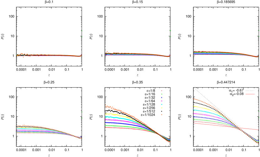
Figure 1: (Colour online). Probability density $P(z)$ for various compressibilities $\beta$: $\beta_{\rm c}=1/\sqrt{29}=0.185\ldots$ is our estimate of the critical compressibility, and $D_{2}=1$ when $\beta=1/\sqrt{5}=0.447\ldots$. Straight lines indicate estimates for $\alpha_{1}$ and $\alpha_{2}$ when $\beta>\beta_{\rm c}$. Note that $P(z)$ is normalisable ($\alpha_{1}>-1$) even at $\beta=1/\sqrt{5}$, where $D_{2}=1$.

The size and shape of a triplet of points $(\mbox{\boldmath$r$}_{0},\mbox{\boldmath$r$}_{1},\mbox{\boldmath$r$}_{2})$ may be described by three parameters: $R_{1}$, $R_{2}$, and $\delta\theta$, which are defined by parametrising the separations $\delta\mbox{\boldmath$r$}_{i}=\mbox{\boldmath$r$}_{i}-\mbox{\boldmath$r$}_{0}$ as follows:

$$\delta\mbox{\boldmath$r$}_{1}=R_{1}{\bf n}_{1}\ ,\ \ \ \delta\mbox{\boldmath$r$}_{2}=R_{2}({\bf n}_{1}+\delta\theta{\bf n}_{2})$$ (4)

where ${\bf n}_{1}$, ${\bf n}_{2}$ are two orthogonal, time dependent unit vectors and the particles are labelled such that $R_{1}\geq R_{2}$. The equations of motion for $R_{1}$, $R_{2}$ and $\delta\theta$ are obtained by substituting (4) into (3) and projecting the equations of motion for $\delta\mbox{\boldmath$r$}_{i}$ onto the ${\bf n}_{j}$. Using the notation

$$F_{ij}={\bf n}_{i}\cdot{\bf A}\,{\bf n}_{j}$$ (5)

we obtain $\dot{\bf n}_{1}\cdot{\bf n}_{2}=F_{21}(t)$,

$$\frac{\dot{R}_{1}}{R_{1}}=F_{11}(t)\ ,\ \ \ \frac{\delta\dot{\theta}}{\delta\theta}=F_{22}(t)-F_{11}(t)$$ (6)

and a similar equation for $\dot{R}_{2}/R_{2}$.

The important point about (6) is that the logarithmic derivative is expressed in terms of the randomly fluctuating quantities $F_{ij}(t)$, so that it is advantageous to transform to logarithmic variables. The variables $(R_{1},R_{2},\delta\theta)$ can be replaced by

$$X_{1}=-{\rm ln}\,\frac{R_{1}}{\xi}\ ,\ \ \ X_{2}=-{\rm ln}\,\delta\theta\ ,\ \ \ X_{3}={\rm ln}\,\left(\frac{R_{1}}{R_{2}}\right)$$ (7)

where $\xi$ is the correlation length of the velocity field. When $X_{1}$ and $X_{2}$ satisfy $X_{1}\gg 0$ and $X_{2}\gg 0$, (that is we are dealing with a small, acute-angled triangles), the dynamics is trivial: $X_{3}$ is frozen and $X_{1}$, $X_{2}$ obey stochastic equations of motion $\dot{X}_{i}=\eta_{i}(t)$, where the $\eta_{i}(t)$ are random functions of time, with statistics independent of position in $(X_{1},X_{2},X_{3})$ space. Because $X_{3}$ is frozen, we have $\eta_{3}(t)=0$. The probability density $P(X_{1},X_{2},X_{3})$ obeys a steady-state advection-diffusion equation, $v_{i}\partial_{i}P+{\cal D}_{ij}\partial_{i}\partial_{j}P=0$ (with $\partial_{i}=\partial/\partial X_{i}$, and summation over repeated indices). The drift velocities, correlation functions and diffusion coefficients are:

$$v_{i}=\langle\dot{X}_{i}(t)\rangle\ \ \ \ \ \ C_{ij}(t)=\langle[\dot{X}_{i}(t)-v_{i}][\dot{X}_{j}(0)-v_{j}]\rangle$$

$${\cal D}_{ij} = \frac{1}{2}\int_{-\infty}^{\infty}{\rm d}t\ C_{ij}(t)\ .$$ (8)

At this point we can already see why $z$ may have a power-law distribution. Note that, because $z\sim\delta\theta$, if $\delta\theta$ has a power-law distribution, then $z$ also has a power-law distribution with the same exponent. Because the equation of motion for $(X_{1},X_{2},X_{3})$ is translationally invariant in the sector $X_{1},X_{2}\gg 0$, any function invariant under translation (up to a change of normalisation) gives a steady-state solution for $P(X_{1},X_{2},X_{3})$. Because the exponential function is translationally invariant, solutions exist in the form $P(X_{1},X_{2},X_{3})=\exp(\gamma_{1}X_{1}+\gamma_{2}X_{2})P_{3}(X_{3})$ (where normalisation requires that the constants $\gamma_{i}$ are negative). The corresponding distributions of $R_{1}$ and $\delta\theta$ have probability densities proportional to $R_{1}^{\gamma_{1}-1}$ and $\delta\theta^{\gamma_{2}-1}$ respectively, so that $P(z)\sim z^{\alpha}$ with $\alpha=\gamma_{2}-1$. Also, we identify $R_{1}$ with $\epsilon$ and note that $\epsilon^{\gamma_{1}}$ is the probability density for both points being within a ball of radius $\epsilon$ surrounding the reference point, implying that $\gamma_{1}=2D_{3}$, where $D_{3}$ is the third Renyi dimension Hal+86 .

In order to identify which power-law solutions obtain we must consider the boundary conditions on the lines $X_{1}=0$ and $X_{2}=0$. The boundary $X_{1}=0$ is a distributed source, corresponding to random triplets of points with a separation approximately equal to the correlation length $\xi$. Some of these are ‘squeezed’ by the linearised flow so that they enter the region $X_{1}>0$. Phase points $X$ representing these triplets are created on the line $X_{1}=0$ at a rate $J(X_{2})$ which corresponds to $\delta\theta$ having a uniform probability density in the limit as $\delta\theta\to 0$ (as required by Kendall’s result Ken77 ), implying that the source density on the boundary $X_{1}=0$ is

$$J(X_{2})=\left\{\begin{array}[]{cc}J_{0}\exp(-X_{2})&X_{2}<0\cr 0&X_{2}\geq 0\end{array}\right.$$ (9)

(where $J_{0}$ is a constant, which determines the normalisation of the joint probability density, $P(X_{1},X_{2},X_{3})$). The boundary at $X_{2}=0$ is more complicated: it is non-absorbing, and the approximations that $X_{3}$ decouples and $(X_{1},X_{2})$ obey a simple diffusion-advection equation fail close to $X_{2}=0$.

It is not possible to determine the steady-state solution of the advection-diffusion equation exactly. In the following we use an approximate propagator to make a quantitative theory for the critical compressibility $\beta_{\rm c}$, and give a qualitative explanation of the reason why there are two exponents, $\alpha_{1}$ and $\alpha_{2}$. Because the probability density is expected to vary over a wide range of values, it is conveniently expressed using an exponential form

$$P(\mbox{\boldmath$X$})\sim\exp\left[-\Phi(\mbox{\boldmath$X$})\right]\ .$$ (10)

Consider first the form of the exponent $\Phi(\mbox{\boldmath$X$})$ for the advection-diffusion equation with drift velocity $v$ and diffusion tensor ${\bf D}$ when there is a point source at the origin. In this case the exponent in (10) will be denoted by $\Phi_{0}(\mbox{\boldmath$X$})$. If the source is localised at $\mbox{\boldmath$X$}={\bf 0}$ and at $t=0$, the solution of the diffusion process in $d$ dimensions is a gaussian centred at $\mbox{\boldmath$X$}=\mbox{\boldmath$v$}t$. The steady-state probability density from a constant intensity source at $\mbox{\boldmath$X$}={\bf 0}$ can be obtained by integration of this gaussian propagator over $t$:

$$P(\mbox{\boldmath$X$}) = K\int_{0}^{\infty}{\rm d}t\ \left[4\pi{\rm det}({\bf D})t\right]^{-d/2}\exp\left[-S(\mbox{\boldmath$X$},t)\right]$$

$$S(\mbox{\boldmath$X$},t) = \frac{1}{4t}(\mbox{\boldmath$X$}-\mbox{\boldmath$v$}t)\cdot{\bf D}^{-1}(\mbox{\boldmath$X$}-\mbox{\boldmath$v$}t)\ .$$ (11)

Here $K$ is a normalisation constant. To estimate $\Phi_{0}(\mbox{\boldmath$X$})$, we determine the time $t^{\ast}$ where the propagator is maximal, and set $\Phi_{0}(\mbox{\boldmath$X$})=S(\mbox{\boldmath$X$},t^{\ast})$, where $\partial S/\partial t(\mbox{\boldmath$X$},t^{\ast})=0$. The equation for $t^{\ast}$ is $\mbox{\boldmath$X$}\cdot{\bf D}^{-1}\mbox{\boldmath$X$}-t^{\ast 2}\mbox{\boldmath$v$}\cdot{\bf D}^{-1}\mbox{\boldmath$v$}=0$. Hence

$$\Phi_{0}(\mbox{\boldmath$X$})=\frac{1}{2}\left[\sqrt{\mbox{\boldmath$X$}\ \cdot{\bf D}^{-1}\mbox{\boldmath$X$}}\sqrt{\mbox{\boldmath$v$}\ \cdot{\bf D}^{-1}\mbox{\boldmath$v$}}-\mbox{\boldmath$X$}\cdot{\bf D}^{-1}\mbox{\boldmath$v$}\right]\ .$$ (12)

Note that $\Phi_{0}(X_{1},X_{2})$ is the height of a tilted conical surface, which touches the $(X_{1},X_{2})$ plane along the ray $\mbox{\boldmath$X$}=\lambda\mbox{\boldmath$v$}$ with parameter $\lambda$ (‘downwind’ of the source), but increases linearly along any other ray starting from the source point. Correspondingly, there is an asymptotically exponential reduction of $P(X_{1},X_{2})$ along any ray from the source.

Next we estimate $P(\mbox{\boldmath$X$})=\exp[-\Phi(\mbox{\boldmath$X$})]$ taking account of the condition that there is a distributed source on the line $X_{2}>0$, with intensity $J(X_{2})=\exp(-X_{2})$. The probability is obtained by integrating the point-source solution $\exp[-\Phi_{0}(\mbox{\boldmath$X$})]$ over the initial point, $(X_{1},X_{2})=(0,X_{0})$, with $X_{0}>0$:

$$P(X_{1},X_{2})=\int_{0}^{\infty}{\rm d}X_{0}\ \exp(-X_{0})\exp[-\Phi_{0}(X_{1},X_{2}-X_{0})]\ .$$ (13)

We may assume that the integral is dominated by contributions from the vicinity of a stationary point $X^{\ast}$. The exponent in (Triangular Constellations in Fractal Measures) is then determined by

$$\Phi(X_{1},X_{2}) = \Phi_{0}(X_{1},X_{2}-X^{\ast})+X^{\ast}$$

$$0 = 1-\frac{\partial\Phi_{0}}{\partial X_{2}}(X_{1},X_{2}-X^{\ast})\ .$$ (14)

Because of the conic structure of the function $\Phi_{0}(X_{1},X_{2})$, the gradient of this function is constant along any ray from the source point $(X_{1},X_{2})=(0,X^{\ast})$. For any given value of the compressibility parameter $\beta$ the stationary point condition is satisfied on a ray which leaves the source point with a slope $s(\beta)$ (which is determined for a specific model below). The stationary point is therefore

$$X^{\ast}=X_{2}-s(\beta)X_{1}\ .$$ (15)

Hence $\Phi(X_{1},X_{2})=\Phi_{0}(X_{1},s(\beta)X_{1})+X_{2}-s(\beta)X_{1}$.

This analysis is only correct if there is a valid stationary point, that is when (15) predicts $X^{\ast}>0$. If $s(\beta)<0$, there is always a positive solution to equation (15), and $\Phi(X_{1},X_{2})\sim X_{2}$, so that $P(z)\sim z^{0}$. If $s(\beta)>0$, however, stationary points (15) do not exist when $(X_{1},X_{2})$ lies below the line of slope $s(\beta)$. In this case the integral (13) is dominated by the contribution from $X_{0}=0$, and we have $\Phi(X_{1},X_{2})\sim\Phi_{0}(X_{1},X_{2})$. In the case where $s(\beta)>0$, there are two exponents ($\alpha_{2}$ and $\alpha_{1}$ respectively) which characterise $P(z)$, depending upon whether $(X_{1},X_{2})=({\rm ln}(\xi/\epsilon),-{\rm ln}(\delta\theta))$ lies above or below the line of slope $s(\beta)$. These exponents are, respectively, $\alpha_{1}=\partial_{X_{2}}\Phi(X_{1},0)-1$, $\alpha_{2}=\lim_{X_{2}\to\infty}\partial_{X_{2}}\Phi(X_{1},X_{2})-1$.

The phase transition illustrated in figure 1 is determined by the condition $s(\beta_{\rm c})=0$. Consider the source of small, non-acute triangles (represented by $X_{1}\gg 1$, $X_{2}\approx 0$). When $\beta<\beta_{\rm c}$, there is a solution of (Triangular Constellations in Fractal Measures) and these triangles are predominantly formed by squeezing of acute triangles from $(0,X^{\ast})$ along their axis. When $\beta>\beta_{\rm c}$, they are formed by approximately isotropic squeezing of non-acute triangles.

We now show how these predictions are illustrated by the numerical results plotted in figure 1. In our numerical investigations we have used the map

$$\mbox{\boldmath{$x$}}_{n+1}=\mbox{\boldmath{$x$}}_{n}+\mbox{\boldmath{$u$}}_{n}(\mbox{\boldmath{$x$}}_{n})\sqrt{\delta t}$$ (16)

with the velocity field $u$ constructed from a stream function $\psi$ and a scalar potential $\phi$:

$$\mbox{\boldmath$u$}_{n}=\left(\partial_{y}\psi_{n}+\beta\partial_{x}\phi_{n},-\partial_{x}\psi_{n}+\beta\partial_{y}\phi_{n}\right)\ .$$ (17)

This is equivalent to using a velocity field which is delta-correlated in time Fal+01 . The timestep $\delta t$ is assumed to be sufficiently small to allow the use of diffusive approximations. The random fields $\phi$ and $\psi$ have the same translationally invariant and isotropic statistics. They are independent of each other and chosen independently at each timestep, and were normalised so that $\langle(\partial_{xy}\psi)^{2}\rangle=1$. For this flow the elements of the diffusion tensor ${\bf D}$ are ${\cal D}_{11}=\frac{1}{2}(1+3\beta^{2})$, ${\cal D}_{12}={\cal D}_{21}=-(1+\beta^{2})$, ${\cal D}_{22}=2(1+\beta^{2})$ and the components of the drift velocity are $v_{1}=1-\beta^{2}$, $v_{2}=-2(1+\beta^{2})$. The correlation dimension is $D_{2}=-v_{1}/{\cal D}_{11}=2(1-\beta^{2})/(1+3\beta^{2})$, Bec+04 ; Wil+12 (so that $D_{2}=1$ for $\beta=1/\sqrt{5}$). Writing $K=(1+3\beta^{2})/(2\beta\sqrt{2(1+\beta^{2})})$, $\Lambda=4(1+\beta^{2})/(1+3\beta^{2})$, the exponent (12) for the point-source solution is

$$\Phi_{0}(\mbox{\boldmath$x$})=K\sqrt{X_{2}^{2}+\Lambda(X_{1}^{2}+X_{1}X_{2})}-X_{1}-X_{2}\ .$$ (18)

Substituting this into (Triangular Constellations in Fractal Measures), we find that the stationary point satisfies (15) with slope

$$s(\beta)=\frac{2(1+\beta^{2})}{1+3\beta^{2}}\left[\frac{8\beta^{2}}{\sqrt{1-26\beta^{2}-23\beta^{4}}}-1\right]$$ (19)

so that $s(\beta)=0$ at $\beta=1/\sqrt{29}=0.185\ldots$, where $D_{2}=7/4$. This implies that $P(z)\sim z^{0}$, independent of $\beta$, for $\beta\leq\beta_{\rm c}=1/\sqrt{29}$. This prediction for the critical compressibility is in good agreement with our numerical results, illustrated in figure 1. When $\beta>1/\sqrt{29}$, the there are two different exponents for $P(z)$ because the dominant contribution to the propagator depends upon the position in the $(X_{1},X_{2})$ plane. We remark that a quantitative treatment of the exponents $\alpha_{1}$, $\alpha_{2}$ when $\beta>\beta_{\rm c}$ requires a more sophisticated model for the propagator, taking account of the different boundary condition at $X_{2}=0$.

In conclusion, we investigated the distribution of shapes of triangular constellations in fractal sets arising from compressible chaotic flow. We find that the distribution of the acute angle is approximately independent of compressibility $\beta$ up to a critical point $\beta_{\rm c}$, which we were able to determine analytically. For $\beta>\beta_{\rm c}$ the exponent $\alpha$ in $P(z)\sim z^{\alpha}$ takes two different values, depending upon how small $z$ is. We thank Alain Pumir for helpful discussions.

References

- (1) J-F. Gouyet, Physics and Fractal Structures, New York: Springer, (1996).
- (2) P. Grassberger and I. Procaccia, Physica D, 13, 34-54, (1984).
- (3) T. C. Halsey, M. H. Jensen, L. P. Kadanoff, I. Procaccia and B. I. Shraiman, Phys. Rev. A, 33, 1141, (1986).
- (4) E. Ott, Chaos in Dynamical Systems, 2nd edition, Cambridge: University Press, (2002).
- (5) J. Sommerer and E. Ott, Science, 359, 334, (1993).
- (6) L. Pietronero, Physica A, 144, 257, (1987).
- (7) D. G. Kendall, Adv. Appl. Prob., 9, 428-30, (1977).
- (8) A. Pumir and M. Wilkinson, J. Stat. Phys., 152, 934-53, 2013.
- (9) G. Falkovich, K. Gawedzki and M. Vergassola, Rev. Mod. Physics , 73, 913-975, (2000).
- (10) J. Bec, K. Gawedzki and P. Horvai, Phys. Rev. Lett., 92, 224501, (2004).
- (11) M. Wilkinson, B. Mehlig, K. Gustavsson and E. Werner, Eur. Phys. J. B, 85, 18, (2012).