The Falling Factorial Basis and Its Statistical Applications

Abstract

We study a novel spline-like basis, which we name the “falling factorial basis”, bearing many similarities to the classic truncated power basis. The advantage of the falling factorial basis is that it enables rapid, linear-time computations in basis matrix multiplication and basis matrix inversion. The falling factorial functions are not actually splines, but are close enough to splines that they provably retain some of the favorable properties of the latter functions. We examine their application in two problems: trend filtering over arbitrary input points, and a higher-order variant of the two-sample Kolmogorov-Smirnov test.

1 Introduction

Splines are an old concept, and they play important roles in various subfields of mathematics and statistics; see e.g., de Boor (1978), Wahba (1990) for two classic references. In words, a spline of order $k$ is a piecewise polynomial of degree $k$ that is continuous and has continuous derivatives of orders $1,2,\ldots k-1$ at its knot points. In this paper, we look at a new twist on an old problem: we examine a novel set of spline-like basis functions with sound computational and statistical properties. This basis, which we call the falling factorial basis, is particularly attractive when assessing higher order of smoothness via the total variation operator, due to the capability for sparse decompositions. A summary of our main findings is as follows.

• The falling factorial basis and its inverse both admit a linear-time transformation, i.e., much faster decompositions than the spline basis, and even faster than, e.g., the fast Fourier transform.

• For all practical purposes, the falling factorial basis shares the statistical properties of the spline basis. We derive a sharp characterization of the discrepancy between the two bases in terms of the polynomial degree and the distance between sampling points.

• We simplify and extend known convergence results on trend filtering, a nonparametric regression technique that implicitly employs the falling factorial basis.

• We also extend the Kolmogorov-Smirnov two-sample test to account for higher order differences, and utilize the falling factorial basis for rapid computations. We provide no theory but demonstrate excellent empirical results, improving on, e.g., the maximum mean discrepancy (Gretton et al., 2012) and Anderson-Darling (Anderson & Darling, 1954) tests.

In short, the falling factorial function class offers an exciting prospect for univariate function regularization.

Now let us review some basics. Recall that the set of $k$th order splines with knots over a fixed set of $n$ points forms an $(n+k+1)$-dimensional subspace of functions. Here and throughout, we assume that we are given ordered input points $x_{1}<x_{2}<\ldots<x_{n}$ and a polynomial order $k\geq 0$, and we define a set of knots $T=\{t_{1},\ldots t_{n-k-1}\}$ by excluding some of the input points at the left and right boundaries, in particular,

$$T=\begin{cases}\{x_{k/2+2},\ldots x_{n-k/2}\}&\text{if $k$ is even},\\ \{x_{(k+1)/2+1},\ldots x_{n-(k+1)/2}\}&\text{if $k$ is odd}.\end{cases}$$ (1.1)

The set of $k$th order splines with knots in $T$ hence forms an $n$-dimensional subspace of functions. The canonical parametrization for this subspace is given by the truncated power basis, $g_{1},\ldots g_{n}$, defined as

$$\begin{gathered}g_{1}(x)=1,\;g_{2}(x)=x,\;\ldots\;g_{k+1}(x)=x^{k},\\ g_{k+1+j}(x)=(x-t_{j})^{k}\cdot 1\{x\geq t_{j}\},\;\;\hfill j=1,\ldots n-k-1.\end{gathered}$$ (1.2)

These functions can also be used to define the truncated power basis matrix, $G\in\mathbb{R}^{n\times n}$, by

$$G_{ij}=g_{j}(x_{i}),\;\;\;i,j=1,\ldots n,$$ (1.3)

i.e., the columns of $G$ give the evaluations of the basis functions $g_{1},\ldots g_{n}$ over the inputs $x_{1},\ldots x_{n}$. As $g_{1},\ldots g_{n}$ are linearly independent functions, $G$ has linearly independent columns, and hence $G$ is invertible.

As noted, our focus is a related but different set of basis functions, named the falling factorial basis functions. We define these functions, for a given order $k\geq 0$, as

$$\begin{gathered}h_{j}(x)=\prod_{\ell=1}^{j-1}(x-x_{\ell}),\;\;\;j=1,\ldots k+1,\\ h_{k+1+j}(x)=\prod_{\ell=1}^{k}(x-x_{j+\ell})\cdot 1\{x\geq x_{j+k}\},\;\;\hfill j=1,\ldots n-k-1.\end{gathered}$$ (1.4)

(Our convention is to take the empty product to be 1, so that $h_{1}(x)=1$.) The falling factorial basis functions are piecewise polynomial, and have an analogous form to the truncated power basis functions in (1.2). Loosely speaking, they are given by replacing an $r$th order power function in the truncated power basis with an appropriate $r$-term product, e.g., replacing $x^{2}$ with $(x-x_{2})(x-x_{1})$, and $(x-t_{j})^{k}$ with $(x-x_{j+k})(x-x_{j+k-1})\cdot\ldots(x-x_{j+1})$. Similar to the above, we can define the falling factorial basis matrix, $H\in\mathbb{R}^{n\times n}$, by

$$H_{ij}=h_{j}(x_{i}),\;\;\;i,j=1,\ldots n,$$ (1.5)

and the linear independence of $h_{1},\ldots h_{n}$ implies that $H$ too is invertible.

Note that the first $k+1$ functions of either basis, the truncated power or falling factorial basis, span the same space (the space of $k$th order polynomials). But this is not true of the last $n-k-1$ functions. Direct calculation shows that, while continuous, the function $h_{j+k+1}$ has discontinuous derivatives of all orders $1,\ldots k$ at the point $x_{j+k}$, for $j=1,\ldots n-k-1$. This means that the falling factorial functions $h_{k+2},\ldots h_{n}$ are not actually $k$th order splines, but are instead continuous $k$th order piecewise polynomials that are “close to” splines. Why would we ever use such a seemingly strange basis as that defined in (1.4)? To repeat what was summarized above, the falling factorial functions allow for linear-time (and closed-form) computations with the basis matrix $H$ and its inverse. Meanwhile, the falling factorial functions are close enough to the truncated power functions that using them in several spline-based problems (i.e., using $H$ in place of $G$) can be statistically legitimized. We make this statement precise in the sections that follow.

As we see it, there is really nothing about their form in (1.4) that suggests a particularly special computational structure of the falling factorial basis functions. Our interest in these functions arose from a study of trend filtering, a nonparametric regression estimator, where the inverse of $H$ plays a natural role. The inverse of $H$ is a kind of discrete derivative operator of order $k+1$, properly adjusted for the spacings between the input points $x_{1},\ldots x_{n}$. It is really the special, banded structure of this derivative operator that underlies the computational efficiency surrounding the falling factorial basis; all of the computational routines proposed in this paper leverage this structure.

Here is an outline for rest of this article. In Section 2, we describe a number of basic properties of the falling factorial basis functions, culminating in fast linear-time algorithms for multiplication $H$ and $H^{-1}$, and tight error bounds between $H$ and the truncated power basis matrix $G$. Section 3 discusses B-splines, which provide another highly efficient basis for spline manipulations; we explain why the falling factorial basis offers a preferred parametrization in some specific statistical applications, e.g., the ones we present in Sections 4 and 5. Section 4 covers trend filtering, and extends a known convergence result for trend filtering over evenly spaced input points (Tibshirani, 2014) to the case of arbitrary input points. The conclusion is that trend filtering estimates converge at the minimax rate (over a large class of true functions) assuming only mild conditions on the inputs. In Section 5, we consider a higher order extension of the classic two-sample Kolmogorov-Smirnov test. We find this test to have better power in detecting higher order (tail) differences between distributions when compared to the usual Kolmogorov-Smirnov test; furthermore, by employing the falling factorial functions, it can computed in linear time. In Section 6, we end with some discussion.

2 Basic properties

Consider the falling factorial basis matrix $H\in\mathbb{R}^{n\times n}$, as defined in (1.5), over input points $x_{1}<\ldots<x_{n}$. The following subsections describe a recursive decomposition for $H$ and its inverse, which lead to fast computational methods for multiplication by $H$ and $H^{-1}$ (as well as $H^{T}$ and $(H^{T})^{-1}$). The last subsection bounds the maximum absolute difference bewteen the elements of $H$ and $G$, the truncated power basis matrix (also defined over $x_{1},\ldots x_{n}$). Lemmas 1, 2, 4 below were derived in Tibshirani (2014) for the special case of evenly spaced inputs, $x_{i}=i/n$ for $i=1,\ldots n$. We reiterate that here we consider generic input points $x_{1},\ldots x_{n}$. In the interest of space, we defer all proofs to the appendix.

2.1 Recursive decomposition

Our first result shows that $H$ decomposes into a product of simpler matrices. It helpful to define, for $k\geq 1$,

$$\Delta^{(k)}=\mathrm{diag}\big{(}x_{k+1}-x_{1},\,x_{k+2}-x_{2},\,\ldots\,x_{n}-x_{n-k}\big{)},$$

the $(n-k)\times(n-k)$ diagonal matrix whose diagonal elements contain the $k$-hop gaps between input points.

Lemma 1.

Let $I_{m}$ denote the $m\times m$ identity matrix, and $L_{m}$ the $m\times m$ lower triangular matrix of 1s. If we write $H^{(k)}$ for the falling factorial basis matrix of order $k$, then in this notation, we have $H^{(0)}=L_{n}$, and for $k\geq 1$,

$$H^{(k)}=H^{(k-1)}\cdot\left[\begin{array}[]{cc}I_{k}&0\\ 0&\Delta^{(k)}L_{n-k}\end{array}\right].$$ (2.1)

Lemma 1 is really a key workhorse behind many properties of the falling factorial basis functions. E.g., it acts as a building block for results to come: immediately, the representation (2.1) suggests both an analogous inverse representation for $H^{(k)}$, and a computational strategy for matrix multiplication by $H^{(k)}$. These are discussed in the next two subsections. We remark that the result in the lemma may seem surprising, as there is not an apparent connection between the falling factorial functions in (1.4) and the recursion in (2.1), which is based on taking cumulative sums at varying offsets (the rightmost matrix in (2.1)). We were led to this result by studying the evenly spaced case; its proof for the present case is considerably longer and more technical, but the statement of the lemma is still quite simple.

2.2 The inverse basis

The result in Lemma 1 clearly also implies a result on the inverse operators, namely, that $(H^{(0)})^{-1}=L_{n}^{-1}$, and

$$(H^{(k)})^{-1}=\left[\begin{array}[]{cc}I_{k}&0\\ 0&L_{n-k}^{-1}(\Delta^{(k)})^{-1}\end{array}\right]\cdot(H^{(k-1)})^{-1}$$ (2.2)

for all $k\geq 1$. We note that

$$L_{m}^{-1}=\left[\begin{array}[]{cccc}1&0&\ldots&0\\ 1&1&\ldots&0\\ \vdots&&&\\ 1&1&\ldots&1\end{array}\right]^{-1}=\left[\begin{array}[]{c}e_{1}^{T}\\ D^{(1)}\end{array}\right],$$ (2.3)

with $e_{1}=(1,0,\ldots 0)\in\mathbb{R}^{m}$ being the first standard basis vector, and $D^{(1)}\in\mathbb{R}^{(m-1)\times m}$ the first discrete difference operator

$$D^{(1)}=\left[\begin{array}[]{rrrrrr}-1&1&0&\ldots&0&0\\ 0&-1&1&\ldots&0&0\\ \vdots&&&&&\\ 0&0&0&\ldots&-1&1\end{array}\right],$$ (2.4)

With this in mind, the recursion in (2.2) now looks like the construction of the higher order discrete difference operators, over the input $x_{1},\ldots x_{n}$. To define these operators, we start with the first order discrete difference operator $D^{(1)}\in\mathbb{R}^{(n-1)\times n}$ as in (2.4), and define the higher order difference discrete operators according to

$$D^{(k+1)}=D^{(1)}\cdot k\cdot(\Delta^{(k)})^{-1}\cdot D^{(k)},$$ (2.5)

for $k\geq 1$. As $D^{(k+1)}\in\mathbb{R}^{(n-k-1)\times n}$, leading matrix $D^{(1)}$ above denotes the $(n-k-1)\times(n-k)$ version of the first order difference operator in (2.4).

To gather intuition, we can think of $D^{(k)}$ as a type of discrete $k$th order derivative operator across the underlying points $x_{1},\ldots x_{n}$; i.e., given an arbitrary sequence $u=(u_{1},\ldots u_{n})\in\mathbb{R}^{n}$ over the positions $x_{1},\ldots x_{n}$, respectively, we can think of $(D^{(k)}u)_{i}$ as the discrete $k$th derivative of the sequence $u$ evaluated at the point $x_{i}$. It is not difficult to see, from its definition, that $D^{(k)}$ is a banded matrix with bandwidth $k+1$. The middle (diagonal) term in (2.5) accounts for the fact that the underlying positions $x_{1},\ldots x_{n}$ are not necessarily evenly spaced. When the input points are evenly spaced, this term contributes only a constant factor, and the difference operators $D^{(k)}$, $k=1,2,3,\ldots$ take a very simple form, where each row is a shifted version of the previous, and the nonzero elements are given by the $k$th order binomial coefficients (with alternating signs); see Tibshirani (2014).

By staring at (2.2) and (2.5), one can see that the falling factorial basis matrices and discrete difference operators are essentially inverses of each other. The story is only slightly more complicated because the difference matrices are not square.

Lemma 2.

If $H^{(k)}$ is the $k$th order falling factorial basis matrix defined over the inputs $x_{1},\ldots x_{n}$, and $D^{(k+1)}$ is the $(k+1)$st order discrete difference operator defined over the same inputs $x_{1}\ldots x_{n}$, then

$$(H^{(k)})^{-1}=\left[\begin{array}[]{c}C\\ \frac{1}{k!}\cdot D^{(k+1)}\end{array}\right],$$ (2.6)

for an explicit matrix $C\in\mathbb{R}^{(k+1)\times n}$. If we let $A_{i}$ denote the $i$th row of a matrix $A$, then $C$ has first row $C_{1}=e_{1}^{T}$, and subsequent rows

$$C_{i+1}=\left[\frac{1}{(i-1)!}\cdot(\Delta^{(i)})^{-1}\cdot D^{(i)}\right]_{1},\;\;\;i=1,\ldots k.$$

Lemma 2 shows that the last $n-k-1$ rows of $(H^{(k)})^{-1}$ are given exactly by $D^{(k+1)}/k!$. This serves as the crucial link between the falling factorial basis functions and trend filtering, discussed in Section 4. The route to proving this result revealed the recursive expressions (2.1) and (2.2), and in fact these are of great computational interest in their own right, as we discuss next.

2.3 Fast matrix multiplication

The recursions in (2.1) and (2.2) allow us to apply $H^{(k)}$ and $(H^{(k)})^{-1}$ with specialized linear-time algorithms. Further, these algorithms are completely in-place: we do not need to form the matrices $H^{(k)}$ or $(H^{(k)})^{-1}$, and the algorithms operate entirely by manipulating the input vector (the vector to be multiplied).

Lemma 3.

For the $k$th order falling factorial basis matrix $H^{(k)}\in\mathbb{R}^{n\times n}$, over arbitrary sorted inputs $x_{1},\ldots x_{n}$, multiplication by $H^{(k)}$ and $(H^{(k)})^{-1}$ can each be computed in $O(nk)$ in-place operations with zero memory requirements (aside from storing the input points and the vector to be multiplied), i.e., we do not need to form $H^{(k)}$ or $(H^{(k)})^{-1}$. Algorithms 1 and 2 give the details. The same is true for matrix multiplication by $(H^{(k)})^{T}$ and $[(H^{(k)})^{T}]^{-1}$; Algorithms 3 and 4, found in the appendix, give the details.

Algorithm 1 Multiplication by $H^{(k)}$

  Input: Vector to be multiplied $y\in\mathbb{R}^{n}$, order $k\geq 0$, sorted inputs vector $x\in\mathbb{R}^{n}$.

  Output: $y$ is overwritten by $H^{(k)}y$.

  for $i=k$ to $0$ do

     $y_{(i+1):n}=\mathrm{cumsum}(y_{(i+1):n})$, where $y_{a:b}$ denotes the subvector $(y_{a},y_{a+1},...,y_{b})$ and $\mathrm{cumsum}$ is the cumulative sum operator.

     if $i\neq 0$ then

        $y_{(i+1):n}=(x_{(i+1):n}-x_{1:(n-i)})\,.*\,y_{(i+1):n}$, where $.*$ denotes entrywise multiplication.

     end if

  end for

  Return $y$.

Algorithm 2 Multiplication by $(H^{(k)})^{-1}$

  Input: Vector to be multiplied $y\in\mathbb{R}^{n}$, order $k\geq 0$, sorted inputs vector $x\in\mathbb{R}^{n}$.

  Output: $y$ is overwritten by $(H^{(k)})^{-1}y$.

  for $i=0$ to $k$ do

     if $i\neq 0$ then

        $y_{(i+1):n}=y_{i+1:n}\,./\,(x_{(i+1):n}-x_{1:(n-i]})$, where $./$ is entrywise division.

     end if

     $y_{(i+2):n}=\mathrm{diff}(y_{(i+1):n})$, where $\mathrm{diff}$ is the pairwise difference operator.

  end for

  Return $y$.

Note that the lemma assumes presorted inputs $x_{1},\ldots x_{n}$ (sorting requires an extra $O(n\log{n})$ operations). The routines for multiplication by $H^{(k)}$ and $(H^{(k)})^{-1}$, in Algorithms 1 and 2, are really just given by inverting each term one at a time in the product representations (2.1) and (2.2). They are composed of elementary in-place operations, like cumulative sums and pairwise differences. This brings to mind a comparison to wavelets, as both the wavelet and inverse wavelets operators can be viewed as highly specialized linear-time matrix multplications.

Borrowing from the wavelet perspective, given a sampled signal $y_{i}=f(x_{i})$, $i=1,\ldots n$, the action $(H^{(k)})^{-1}y$ can be thought of as the forward transform under the piecewise polynomial falling factorial basis, and $H^{(k)}y$ as the backward or inverse transform under this basis. It might be interesting to consider the applicability of such transforms to signal processing tasks, but this is beyond the scope of the current paper, and we leave it to potential future work.

We do however include a computational comparison between the forward and backward falling factorial transforms, in Algorithms 2 and 1, and the well-studied Fourier and wavelet transforms. Figure 1(a) shows the runtimes of one complete cycle of falling factorial transforms (i.e., one forward and one backward transform), with $k=3$, versus one cycle of fast Fourier transforms and one cycle of wavelet transforms (using symmlets). The comparison was run in Matlab, and we used Matlab’s “fft” and “ifft” functions for the fast Fourier transforms, and the Stanford WaveLab’s “FWT_PO” and “IWT_PO” functions (with symmlet filters) for the wavelet transforms (Buckheit & Donoho, 1995). These functions all call on C implementations that have been ported to Matlab using MEX-functions, and so we did the same with our falling factorial transforms to even the comparison. For each problem size $n$, we chose evenly spaced inputs (this is required for the Fourier and wavelet transforms, but recall, not for the falling factorial transform), and averaged the results over 10 repetitions. The figure clearly demonstrates a linear scaling for the runtimes of the falling factorial transform, which matches their theoretical $O(n)$ complexity; the wavelet and fast fourier transforms also behave as expected, with the former having $O(n)$ complexity, and the latter $O(n\log{n})$. In fact, a raw comparison of times shows that our implementation of the falling factorial transforms runs slightly faster than the highly-optimized wavelet transforms from the Stanford WaveLab.

For completeness, Figure 1(b) displays a comparison between the falling factorial transforms and the corresponding transforms using the truncated power basis (also with $k=3$). We see that the latter scale quadratically with $n$, which is again to be expected, as the truncated power basis matrix is essentially lower triangular.

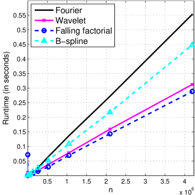
(a) Falling factorial vs. Fourier, wavelet, and B-spline transforms (linear scale)

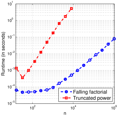
(b) Falling factorial (H) vs. truncated power (G) transforms (log-log scale)

Figure 2.1: Comparison of runtimes for different transforms. The experiments were performed on a laptop computer.

2.4 Proximity to truncated power basis

With computational efficiency having been assured by the last lemma, our next lemma lays the footing for the statistical credibility of the falling factorial basis.

Lemma 4.

Let $G^{(k)}$ and $H^{(k)}$ be the $k$th order truncated power and falling factorial matrices, defined over inputs $0\leq x_{1}<\ldots<x_{n}\leq 1$. Let $\delta=\max_{i=1,\ldots n}(x_{i}-x_{i-1})$, where we write $x_{0}=0$. Then

$$\max_{i,j=1,\ldots n}\,|G^{(k)}_{ij}-H^{(k)}_{ij}|\leq k^{2}\delta.$$

This tight elementwise bound between the two basis matrices will be used in Section 4 to prove a result on the convergence of trend filtering estimates. We will also discuss its importance in the context of a fast nonparametric two-sample test in Section 5. To give a preview: in many problem instances, the maximum gap $\delta$ between adjacent sorted inputs $x_{1},\ldots x_{n}$ is of the order $\log{n}/n$ (for a more precise statement see Lemma 5), and this means that the maximum absolute discrepancy between the elements of $G^{(k)}$ and $H^{(k)}$ decays very quickly.

3 Why not just use B-splines?

B-splines already provide a computationally efficient parametrization for the set of $k$th order splines; i.e., since they produce banded basis matrices, we can already perform linear-time basis matrix multiplication and inversion with B-splines. To confirm this point empirically, we included B-splines in the timing comparison of Section 2.3, refer to Figure 1(a) for the results. So, why not always use B-splines in place of the falling factorial basis, which only approximately spans the space of splines?

A major reason is that the falling factorial functions (like the truncated power functions) admit a sparse representation under the total variation operator, whereas the B-spline functions do not. To be more specific, suppose that $f_{1},\ldots f_{m}$ are $k$th order piecewise polynomial functions with knots at the points $0\leq z_{1}<\ldots<z_{r}\leq 1$, where $m=r+k+1$. Then, for $f=\sum_{j=1}^{m}\alpha_{j}f_{j}$, we have

$$\mathrm{TV}(f^{(k)})=\sum_{i=1}^{r}\left|\sum_{j=1}^{m}\left(f_{j}^{(k)}(z_{i})-f_{j}^{(k)}(z_{i-1})\right)\cdot\alpha_{j}\right|,$$

denoting $z_{0}=0$ for ease of notation. If $f_{1},\ldots f_{m}$ are the falling factorial functions defined over the points $z_{1},\ldots z_{r}$, then the term $f_{j}^{(k)}(z_{i})-f_{j}^{(k)}(z_{i-1})$ is equal to 0 for all $i,j$, except when $i=j-k-1$ and $j\geq k+2$, in which case it equals 1. Therefore, $\mathrm{TV}(f^{(k)})=\sum_{j=k+2}^{m}|\alpha_{j}|$, a simple sum of absolute coefficients in the falling factorial expansion. The same result holds for the truncated power basis functions. But if $f_{1},\ldots f_{m}$ are B-splines, then this is not true; one can show that in this case $\mathrm{TV}(f^{(k)})=\|C\alpha\|_{1}$, where $C$ is a (generically) dense matrix. The fact that $C$ is dense makes it cumbersome, both mathematically and computationally, to use the B-spline parametrization in spline problems involving total variation, such as those discussed in Sections 4 and 5.

4 Trend filtering for arbitrary inputs

Trend filtering is a relatively new method for nonparametric regression. Suppose that we observe

$$y_{i}=f_{0}(x_{i})+\epsilon_{i},\;\;\;i=1,\ldots n,$$ (4.1)

for a true (unknown) regression function $f_{0}$, inputs $x_{1}<\ldots<x_{n}\in\mathbb{R}$, and errors $\epsilon_{1},\ldots\epsilon_{n}$. The trend filtering estimator was first proposed by Kim et al. (2009), and further studied by Tibshirani (2014). In fact, the latter work motivated the current paper, as it derived properties of the falling factorial basis over evenly spaced inputs $x_{i}=i/n$, $i=1,\ldots n$, and use these to prove convergence rates for trend filtering estimators. In the present section, we allow $x_{1},\ldots x_{n}$ to be arbitrary, and extend the convergence guarantees for trend filtering, utilizing the properties of the falling factorial basis derived in Section 2.

The trend filtering estimate $\hat{\beta}$ of order $k\geq 0$ is defined by

$$\hat{\beta}=\mathop{\mathrm{argmin}}_{\beta\in\mathbb{R}^{n}}\,\frac{1}{2}\|y-\beta\|_{2}^{2}+\lambda\cdot\frac{1}{k!}\|D^{(k+1)}\beta\|_{1},$$ (4.2)

where $y=(y_{1},\ldots y_{n})\in\mathbb{R}^{n}$, $D^{(k+1)}\in\mathbb{R}^{(n-k-1)\times n}$ is the $(k+1)$st order discrete difference operator defined in (2.5) over the input points $x_{1},\ldots x_{n}$, and $\lambda\geq 0$ is a tuning parameter. We can think of the components of $\hat{\beta}$ as defining an estimated function $\hat{f}$ over the input points. To give an example, in Figure 4.1, we drew noisy observations from a smooth underlying function, where the input points $x_{1},\ldots x_{n}$ were sampled uniformly at random over $[0,1]$, and we computed the trend filtering estimate $\hat{\beta}$ with $k=3$ and a particular choice of $\lambda$. From the plot (where we interpolated between $(x_{1},\hat{\beta}_{1}),\ldots(x_{n},\hat{\beta}_{n})$ for visualization purposes), we can see that the implicitly defined trend filtering function $\hat{f}$ displays a piecewise cubic structure, with adaptively chosen knot points. Lemma 2 makes this connection precise by showing that such a function $\hat{f}$ is indeed a linear combination of falling factorial functions. Letting $\beta=H^{(k)}\alpha$, where $H^{(k)}\in\mathbb{R}^{n\times n}$ is the $k$th order falling factorial basis matrix defined over the inputs $x_{1},\ldots x_{n}$, the trend filtering problem in (4.2) becomes

$$\hat{\alpha}=\mathop{\mathrm{argmin}}_{\alpha\in\mathbb{R}^{n}}\,\frac{1}{2}\|y-H^{(k)}\alpha\|_{2}^{2}+\lambda\cdot\sum_{j=k+2}^{n}|\alpha_{j}|,$$ (4.3)

equivalent to the functional minimization problem

$$\hat{f}=\mathop{\mathrm{argmin}}_{f\in\mathcal{H}_{k}}\,\frac{1}{2}\sum_{i=1}^{n}\big{(}y_{i}-f(x_{i})\big{)}^{2}+\lambda\cdot\mathrm{TV}\big{(}f^{(k)}),$$ (4.4)

where $\mathcal{H}_{k}=\mathrm{span}\{h_{1},\ldots h_{n}\}$ is the span of the $k$th order falling factorial functions in (1.4), $\mathrm{TV}(\cdot)$ denotes the total variation operator, and $f^{(k)}$ denotes the $k$th weak derivative of $f$. In other words, the solutions of problems (4.2) and (4.4) are related by $\hat{\beta}_{i}=\hat{f}(x_{i})$, $i=1,\ldots n$. The trend filtering estimate hence verifiably exhibits the structure of a $k$th order piecewise polynomial function, with knots at a subset of $x_{1},\ldots x_{n}$, and this function is not necessarily a spline, but is close to one (since it lies in the span of the falling factorial functions $h_{1},\ldots h_{n}$).

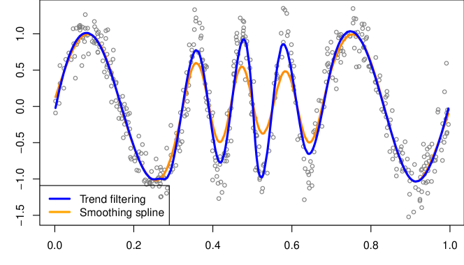
Figure 4.1: Example trend filtering and smoothing spline estimates.

In Figure 4.1, we also fit a smoothing spline estimate to the same example data. A striking difference: the trend filtering estimate is far more locally adaptive towards the middle of plot, where the underlying function is less smooth (the two estimates were tuned to have the same degrees of freedom, to even the comparison). This phenomenon is investigated in Tibshirani (2014), where it is shown that trend filtering estimates attain the minimax convergence rate over a large class of underlying functions, a class for which it is known that smoothing splines (along with any other estimator linear in $y$) are suboptimal. This latter work focused on evenly spaced inputs, $x_{i}=i/n$, $i=1,\ldots n$, and the next two subsections extend the trend filtering convergence theory to cover arbitrary inputs $x_{1},\ldots x_{n}\in[0,1]$. We first consider the input points as fixed, and then random. All proofs are deferred until the appendix.

4.1 Fixed input points

The following is our main result on trend filtering.

Theorem 1.

Let $y\in\mathbb{R}^{n}$ be drawn from (4.1), with fixed inputs $0\leq x_{1}<\ldots<x_{n}\leq 1$, having a maximum gap

$$\max_{i=1,\ldots n}\,(x_{i}-x_{i-1})=O(\log{n}/n),$$ (4.5)

and i.i.d., mean zero sub-Gaussian errors. Assume that, for an integer $k\geq 0$ and constant $C>0$, the true function $f_{0}$ is $k$ times weakly differentiable, with $\mathrm{TV}(f_{0}^{(k)})\leq C$. Then the $k$th order trend filtering estimate $\hat{\beta}$ in (4.2), with tuning parameter value $\lambda=\Theta(n^{1/(2k+3)})$, satisfies

$$\frac{1}{n}\sum_{i=1}^{n}\big{(}\hat{\beta}_{i}-f_{0}(x_{i})\big{)}^{2}=O_{\mathbb{P}}(n^{-(2k+2)/(2k+3)}).$$ (4.6)

Remark 1. The rate $n^{-(2k+2)/(2k+3)}$ is the minimax rate of convergence with respect to the class of $k$ times weakly differentiable functions $f$ such that $\mathrm{TV}(f^{(k)})\leq C$ (see, e.g., Nussbaum (1985), Tibshirani (2014)). Hence Theorem 1 shows that trend filtering estimates converge at the minimax rate over a broad class of true functions $f_{0}$, assuming that the fixed input points are not too irregular, in that the maximum adjacent gap between points must satisfy (4.5). This condition is not stringent and is naturally satisfied by continuously distributed random inputs, as we show in the next subsection. We note that Tibshirani (2014) proved the same conclusion (as in Theorem 1) for unevenly spaced inputs $x_{1},\ldots x_{n}$, but placed very complicated and basically uninterpretable conditions on the inputs. Our tighter analysis of the falling factorial functions yields the simple sufficient condition (4.5).

Remark 2. The conclusion in the theorem can be strengthened, beyond the the convergence of $\hat{\beta}$ to $f_{0}$ in (4.6); under the same assumptions, the trend filtering estimate $\hat{\beta}$ also converges to $\hat{f}^{\mathrm{spline}}$ at the same rate $n^{-(2k+2)/(2k+3)}$, where we write $\hat{f}^{\mathrm{spline}}$ to denote the solution in (4.4) with $\mathcal{H}_{k}$ replaced by $\mathcal{G}_{k}=\mathrm{span}\{g_{1},\ldots g_{n}\}$, the span of the truncated power basis functions in (1.2). This asserts that the trend filtering estimate is indeed “close to” a spline, and here the bound in Lemma 4, between the truncated power and falling factorial basis matrices, is key. Moreover, we actually rely on the convergence of $\hat{\beta}$ to $\hat{f}^{\mathrm{spline}}$ to establish (4.6), as the total variation regularized spline estimator $\hat{f}^{\mathrm{spline}}$ is already known to converge to $f_{0}$ at the minimax rate (Mammen & van de Geer, 1997).

4.2 Random input points

To analyze trend filtering for random inputs, $x_{1},\ldots x_{n}$, we need to bound the maximum gap between adjacent points with high probability. Fortunately, this is possible for a large class of distributions, as shown in the next lemma.

Lemma 5.

If $0\leq x_{1}<\ldots<x_{n}\leq 1$ are sorted i.i.d. draws from an arbitrary continuous distribution supported on $[0,1]$, whose density is bounded below by $p_{0}>0$, then with probability at least $1-2p_{0}n^{-10}$,

$$\max_{i=1,\ldots n}\,(x_{i}-x_{i-1})\leq\frac{c_{0}\log n}{p_{0}n},$$

for a universal constant $c_{0}$.

The proof of this result is readily assembled from classical results on order statistics; we give a simple alternate proof in the appendix. Lemma 5 implies the next corollary.

Corollary 1.

Let $y\in\mathbb{R}^{n}$ be distributed according to the model (4.1), where the inputs $0\leq x_{1}<\ldots<x_{n}\leq 1$ are sorted i.i.d. draws from an arbitrary continuous distribution on $[0,1]$, whose density is bounded below. Assume again that the errors are i.i.d., mean zero sub-Gaussian variates, independent of the inputs, and that the true function $f_{0}$ has $k$ weak derivatives and satisfies $\mathrm{TV}(f_{0}^{(k)})\leq C$. Then, for $\lambda=\Theta(n^{1/(2k+3)})$, the $k$th order trend filtering estimate $\hat{\beta}$ converges at the same rate as in Theorem 1.

5 A higher order Kolmogorov-Smirnov test

The two-sample Kolmogorov-Smirnov (KS) test is a standard nonparametric hypothesis test of equality between two distributions, say $\mathbb{P}_{X}$ and $\mathbb{P}_{Y}$, from independent samples $x_{1},\ldots x_{m}\sim\mathbb{P}_{X}$ and $y_{1},\ldots y_{n}\sim\mathbb{P}_{Y}$. Writing $X_{(m)}=(x_{1},\ldots x_{m})$, $Y_{(n)}=(y_{1},\ldots y_{n})$, and $Z_{(m+n)}=(z_{1},\ldots z_{m+n})=X_{(m)}\cup Y_{(n)}$ for the joined samples, the KS statistic can be expressed as

$$\mathrm{KS}(X_{(m)},Y_{(n)})=\max_{z_{j}\in Z_{(m+n)}}\,\left|\frac{1}{m}\sum_{i=1}^{m}1\{x_{i}\leq z_{j}\}-\frac{1}{n}\sum_{i=1}^{n}1\{y_{i}\leq z_{j}\}\right|.$$ (5.1)

This examines the maximum absolute difference between the empirical cumulative distribution functions from $X_{(m)}$ and $Y_{(n)}$, across all points in the joint set $Z_{(m+n)}$, and so the test rejects for large values of (5.1). A well-known alternative (variational) form for the KS statistic is

$$\mathrm{KS}(X_{(m)},Y_{(n)})=\max_{f\,:\,\mathrm{TV}(f)\leq 1}\,\left|\hat{\mathbb{E}}_{X_{(m)}}[f(X)]-\hat{\mathbb{E}}_{Y_{(n)}}[f(Y)]\right|,$$ (5.2)

where $\hat{\mathbb{E}}_{X_{(m)}}$ denotes the empirical expectation under $X_{(m)}$, so that $\hat{\mathbb{E}}_{X_{(m)}}[f(X)]=1/m\sum_{i=1}^{m}f(x_{i})$, and similarly for $\hat{\mathbb{E}}_{Y_{(n)}}$. The equivalence between (5.2) and (5.1) comes from the fact that maximum in (5.2) is achieved by taking $f$ to be a step function, with its knot (breakpoint) at one of the joined samples $z_{1},\ldots z_{m+n}$.

The KS test is perhaps one of the most widely used nonparametric tests of distributions, but it does have its shortcomings. Loosely speaking, it is known to be sensitive in detecting differences between the centers of distributions $\mathbb{P}_{X}$ and $\mathbb{P}_{Y}$, but much less sensitive in detecting differences in the tails. In this section, we generalize the KS test to “higher order” variants that are more powerful than the original KS test in detecting tail differences (when, of course, such differences are present). We first define the higher order KS test, and describe how it can be computed in linear time with the falling factorial basis. We then empirically compare these higher order versions to the original KS test, and several other commonly used nonparametric two-sample tests of distributions.

5.1 Definition of the higher order KS tests

For a given order $k\geq 0$, we define the $k$th order KS test statistic between $X_{(m)}$ and $Y_{(n)}$ as

$$\mathrm{KS}_{G}^{(k)}(X_{(m)},Y_{(n)})=\left\|(G_{2}^{(k)})^{T}\left(\frac{\mathds{1}_{X_{(m)}}}{m}-\frac{\mathds{1}_{Y_{(n)}}}{n}\right)\right\|_{\infty}.$$ (5.3)

Here $G^{(k)}\in\mathbb{R}^{(m+n)\times(m+n)}$ is the $k$th order truncated power basis matrix over the joined samples $z_{1}<\ldots<z_{m+n}$, assumed sorted without a loss of generality, and $G_{2}^{(k)}$ is the submatrix formed by excluding its first $k+1$ columns. Also, $\mathds{1}_{X_{(m)}}\in\mathbb{R}^{(m+n)}$ is a vector whose components indicate the locations of $x_{1}<\ldots<x_{m}$ among $z_{1}<\ldots<z_{m+n}$, and similarly for $\mathds{1}_{Y_{(n)}}$. Finally, $\|\cdot\|_{\infty}$ denotes the $\ell_{\infty}$ norm, $\|u\|_{\infty}=\max_{i=i,\ldots r}|u_{i}|$ for $u\in\mathbb{R}^{r}$.

As per the spirit of our paper, an alternate definition for the $k$th order KS statistic uses the falling factorial basis,

$$\mathrm{KS}_{H}^{(k)}(X_{(m)},Y_{(n)})=\left\|(H_{2}^{(k)})^{T}\left(\frac{\mathds{1}_{X_{(m)}}}{m}-\frac{\mathds{1}_{Y_{(n)}}}{n}\right)\right\|_{\infty},$$ (5.4)

where now $H^{(k)}\in\mathbb{R}^{(m+n)\times(m+n)}$ is the $k$th order falling factorial basis matrix over the joined samples $z_{1}<\ldots<z_{m+n}$. Not surprisingly, the two definitions are very close, and Hölder’s inequality shows that

$$|\mathrm{KS}_{G}^{(k)}(X_{(m)},Y_{(n)})-\mathrm{KS}_{H}^{(k)}(X_{(m)},Y_{(n)})|\leq\max_{i,j=1,\ldots m+n}\,2|G^{(k)}_{ij}-H^{(k)}_{ij}|\leq 2k^{2}\delta,$$

the last inequality due to Lemma 4, with $\delta$ the maximum gap between $z_{1},\ldots z_{m+n}$. Recall that Lemma 5 shows $\delta$ to be of the order $\log(m+n)/(m+n)$ for continuous distributions $\mathbb{P}_{X},\mathbb{P}_{Y}$ supported nontrivially on $[0,1]$, which means that with high probability, the two definitions differ by at most $2k^{2}\log(m+n)/(m+n)$, in such a setup.

The advantage to using the falling factorial definition is that the test statistic in (5.4) can be computed in $O(k(m+n))$ time, without even having to form the matrix $H^{(k)}_{2}$ (this is assuming sorted points $z_{1},\ldots z_{m+n}$). See Lemma 3, and Algorithm 3 in the appendix. By comparison, the statistic in (5.3) requires $O((m+n)^{2})$ operations. In addition to the theoretical bound described above, we also find empirically that the two definitions perform quite similarly, as shown in the next subsection, and hence we advocate the use of $\mathrm{KS}^{(k)}_{H}$ for computational reasons.

A motivation for our proposed tests is as follows: it can be shown that (5.3), and therefore (5.4), approximately take a variational form similar to (5.2), but where the constraint is over functions whose $k$th (weak) derivative has total variation at most 1. See the appendix.

5.2 Numerical experiments

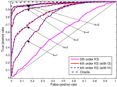
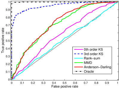
Figure 5.1: ROC curves for experiment 1, normal vs. t.

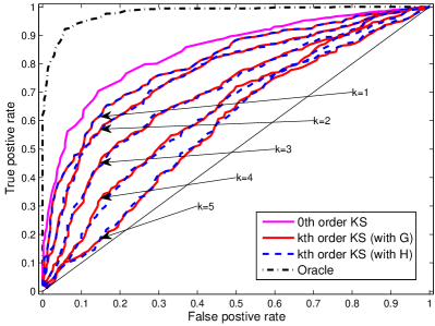
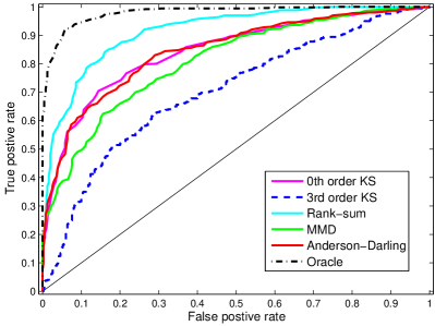
Figure 5.2: ROC curves for experiment 2, Laplace vs. Laplace.

We examine the higher order KS tests by simulation. The setup: we fix two distributions $P,Q$. We draw $n$ i.i.d. samples $X_{(n)},Y_{(n)}\sim P$, calculate a test statistic, and repeat this $R/2$ times; we also draw $n$ i.i.d. samples $X_{(n)}\sim P$, $Y_{(n)}\sim Q$, calculate a test statistic, and repeat $R/2$ times. We then construct an ROC curve, i.e., the true positive rate versus the false positive rate of the test, as we vary its rejection threshold. For the test itself, we consider our $k$th order KS test, in both its $G$ and $H$ forms, as well as the usual KS test, and a number of other popular two-sample tests: the Anderson-Darling test (Anderson & Darling, 1954; Scholz & Stephens, 1987), the Wilcoxon rank-sum test (Wilcoxon, 1945), and the maximum mean discrepancy (MMD) test, with RBF kernel (Gretton et al., 2012).

Figures 5.1 and 5.2 show the results of two experiments in which $n=100$ and $R=1000$. (See the appendix for more experiments.) In the first we used $P=N(0,1)$ and $Q=t_{3}$ ($t$-distribution with 3 degrees of freedom), and in the second $P=\mathrm{Laplace}(0)$ and $Q=\mathrm{Laplace}(0.3)$ (Laplace distributions of different means). We see that our proposed $k$th order KS test performs favorably in the first experiment, with its power increasing with $k$. When $k=3$, it handily beats all competitors in detecting the difference between the standard normal distribution and the heavier-tailed $t$-distribution. But there is no free lunch: in the second experiment, where the differences between $P,Q$ are mostly near the centers of the distributions and not in the tails, we can see that increasing $k$ only decreases the power of the $k$th order KS test. In short, one can view our proposal as introducing a family of tests parametrized by $k$, which offer a tradeoff in center versus tail sensitivity. A more thorough study will be left to future work.

6 Discussion

We formally proposed and analyzed the spline-like falling factorial basis functions. These basis functions admit attractive computational and statistical properties, and we demonstrated their applicability in two problems: trend filtering, and a novel higher order variant of the KS test. These examples, we feel, are just the beginning. As typical operations associated with the falling factorial basis scale merely linearly with the input size (after sorting), we feel that this basis may be particularly well-suited to a rich number of large-scale applications in the modern data era, a direction that we are excited to pursue in the future.

Acknowledgements The research was partially supported by NSF Grant DMS-1309174, Google Faculty Research Grant and the Singapore National Research Foundation under its International Research Centre @ Singapore Funding Initiative and administered by the IDM Programme Office.

This appendix contains proofs and additional experiments for the paper “The Falling Factorial Basis and Its Statistical Applications”. In Section A, we provide proofs to the key technical results in the main paper. In Section B, we give some motivating arguments and additional experiments for the higher order KS test.

Appendix A Proofs and technical details

A.1 Proof of Lemma 1 (recursive decomposition)

The falling factorial basis matrix, as defined in (1.4), (1.5), can be expressed as $H^{(k)}=[H^{(k)}_{1}\,H^{(k)}_{2}]$, where

$$H^{(k)}_{1}=\left[\begin{array}[]{ccccc}1&0&0&\cdots&0\\ 1&x_{2}-x_{1}&0&\cdots&0\\ 1&x_{3}-x_{1}&(x_{3}-x_{2})(x_{3}-x_{1})&\cdots&\vdots\\ \vdots&\vdots&\vdots&\ddots&\vdots\\ 1&x_{k+1}-x_{1}&(x_{k+1}-x_{2})(x_{k+1}-x_{1})&\cdots&\prod_{\ell=1}^{k}(x_{k+1}-x_{\ell})\\ \vdots&\vdots&\vdots&\ddots&\vdots\\ 1&x_{n}-x_{1}&(x_{n}-x_{2})(x_{n}-x_{1})&\cdots&\prod_{\ell=1}^{k}(x_{n}-x_{\ell})\\ \end{array}\right]\in\mathbb{R}^{n\times(k+1)},$$

and

$$H^{(k)}_{2}=\left[\begin{array}[]{cccc}0_{(k+1)\times 1}&0_{(k+1)\times 1}&\cdots&0_{(k+1)\times 1}\\ \prod_{\ell=1}^{k}(x_{k+2}-x_{1+\ell})&0&\cdots&0\\ \prod_{\ell=1}^{k}(x_{k+3}-x_{1+\ell})&\prod_{\ell=1}^{k}(x_{k+3}-x_{2+\ell})&\cdots&0\\ \vdots&\vdots&\ddots&\vdots\\ \prod_{\ell=1}^{k}(x_{n}-x_{1+\ell})&\prod_{\ell=1}^{k}(x_{n}-x_{2+\ell})&\cdots&\prod_{\ell=1}^{k}(x_{n}-x_{n-k-1+\ell})\\ \end{array}\right]\in\mathbb{R}^{n\times(n-k-1)}.$$

Lemma 1 claims that $H^{(0)}=L_{n}$, the lower triangular matrix of $1$s, which can be seen directly by inspection (recalling our convention of defining thee empty product to be 1). The lemma further claims that $H^{(k)}$ can be recursively factorized into the following form:

$$H^{(k)}=H^{(k-1)}\cdot\left[\begin{array}[]{cc}I_{k}&0\\ 0&\Delta^{(k)}\end{array}\right]\cdot\left[\begin{array}[]{cc}I_{k}&0\\ 0&L_{n-k}\end{array}\right],$$ (A.1)

for all $k\geq 1$. We prove the above factorization in this current section. In what follows, we denote the last $n-k-1$ columns of the product (A.1) by $\tilde{M}^{(k)}\in\mathbb{R}^{n\times(n-k-1)}$, and also write

$$\tilde{M}^{(k)}=\left[\begin{array}[]{c}0_{(k+1)\times(n-k-1)}\vskip 3.0pt plus 1.0pt minus 1.0pt\\ \tilde{L}^{(k)},\end{array}\right],$$

i.e., we use $\tilde{L}^{(k)}$ to denote the lower $(n-k-1)\times(n-k-1)$ submatrix of $\tilde{M}^{(k)}$. To prove the lemma, we show that $\tilde{M}^{(k)}$ is equal to the corresponding block $H^{(k)}_{2}$, by induction on $k$. The proof that the first block of $k+1$ columns of the product is equal to $H^{(k)}_{1}$ follows from the arguments given for the proof of the second block, and therefore we do not explicitly rewrite the proof for this part.

We begin the inductive proof by checking the case $k=1$. Note

$$\tilde{M}^{(1)}=\left[\begin{array}[]{c}0_{2\times(n-2)}\vskip 3.0pt plus 1.0pt minus 1.0pt\\ \tilde{L}^{(1)}\end{array}\right] =\left[\begin{array}[]{c}0_{1\times(n-1)}\\ L_{n-1}\end{array}\right](\Delta^{(k)})^{-1}\left[\begin{array}[]{c}0_{1\times(n-2)}\\ L_{n-2}\\ \end{array}\right]$$ (A.8)

$$=\left[\begin{array}[]{cccc}0_{2\times 1}&0_{2\times 1}&\cdots&0_{2\times 1}\\ x_{3}-x_{2}&0&\cdots&0\\ x_{4}-x_{2}&x_{4}-x_{3}&\cdots&0\\ \vdots&\vdots&\ddots&\vdots\\ x_{n}-x_{2}&x_{n}-x_{3}&\cdots&x_{n}-x_{n-1}\end{array}\right].$$ (A.14)

This gives precisely the last $n-2$ columns of $H^{(1)}$, as defined in (1.4).

Next we verify that if the statement holds for some $k\geq 1$, then it is true for $k+1$. To avoid confusion, we will use $i,j$ as indices $H^{(k+1)}$ and $\alpha,\beta$ as indices of $\tilde{L}^{(k+1)}$. The universal rule for the relationship between the two sets of indices is

$$\begin{pmatrix}i\\ j\\ \end{pmatrix}=\begin{pmatrix}\alpha\\ \beta\\ \end{pmatrix}+k+2.$$

We consider an arbitrary element, $\tilde{L}^{(k+1)}_{\alpha\beta}$. Due to the upper triangular shape of $\tilde{L}^{(k)}$, we have $\tilde{L}^{(k)}_{\alpha\beta}=0$ if $\alpha<\beta$. For $\alpha\geq\beta$, we plainly calculate, using the inductive hypothesis

$$\tilde{L}^{(k+1)}_{\alpha\beta} =\sum_{q=1+\beta}^{1+\alpha}\tilde{L}^{(k)}_{1+\alpha,q}\cdot(\Delta^{(k+1)})^{-1}_{qq}$$

$$=\sum_{q=1+\beta}^{1+\alpha}\prod_{\ell=1}^{k}(x_{k+2+\alpha}-x_{q+\ell})\cdot(x_{k+1+q}-x_{q})$$

$$=\prod_{\ell=1}^{k+1}(x_{k+2+\alpha}-x_{\beta+\ell})\cdot A=H^{(k)}_{ij}\cdot A,$$

where $A$ is the sum of terms that scales each summand to the desired quantity (by multiplying and dividing by missing factors). To complete the inductive proof, it suffices to show that $A=1$. It turns out that there are two main cases to consider, which we examine below.

Case 1. When $\alpha-\beta\leq k$, the term $A$ can be expressed as

$$A= \frac{x_{k+1+1+\beta}-x_{1+\beta}}{x_{k+2+\alpha}-x_{1+\beta}}+\frac{(x_{k+1+2+\beta}-x_{2+\beta})(x_{k+2+\alpha}-x_{k+1+1+\beta})}{(x_{k+2+\alpha}-x_{1+\beta})(x_{k+2+\alpha}-x_{2+\beta})}$$

$$+\cdots+\frac{(x_{k+1+\gamma+\beta}-x_{\gamma+\beta})(x_{k+2+\alpha}-x_{k+2+\beta})\cdots(x_{k+2+\alpha}-x_{k+\gamma+\beta})}{(x_{k+2+\alpha}-x_{1+\beta})\cdots(x_{k+2+\alpha}-x_{\gamma-1+\beta})(x_{k+2+\alpha}-x_{\gamma+\beta})}$$

$$+\cdots+\frac{(x_{k+1+\alpha}-x_{\alpha})(x_{k+2+\alpha}-x_{k+2+\beta})\cdots(x_{k+2+\alpha}-x_{k+1+\alpha})}{(x_{k+2+\alpha}-x_{1+\beta})\cdots(x_{k+2+\alpha}-x_{\alpha-1})(x_{k+2+\alpha}-x_{\alpha})}$$

$$+\frac{\cancel{(x_{k+2+\alpha}-x_{1+\alpha})}(x_{k+2+\alpha}-x_{k+2+\beta})\cdots(x_{k+2+\alpha}-x_{k+1+\alpha})}{(x_{k+2+\alpha}-x_{1+\beta})\cdots(x_{k+2+\alpha}-x_{\alpha})\cancel{(x_{k+2+\alpha}-x_{1+\alpha})}}.$$

Note that in the last term, the factor $(x_{k+2+\alpha}-x_{1+\alpha})$ in both the denominator and numerator cancels out, leaving the denominator to be the same as the second to last term. Combining the last two terms, we again get a common factor $(x_{k+2+\alpha}-x_{\alpha})$ in denominator and numerator, which cancels out, and makes the denominator of this term the same as that previous term. Continuing in this manner, we can recursively eliminate the terms from last to the first, leaving

$$\frac{\cancel{x_{k+2+\beta}}-x_{1+\beta}+x_{k+2+\alpha}-\cancel{x_{k+2+\beta}}}{x_{k+2+\alpha}-x_{1+\beta}}=1.$$

In other words, we have shown that $A=1$.

Case 2. When $\alpha-\beta\geq k+1$, the denominators in terms of $A$ will remain the same after they reach

$$(x_{k+2+\alpha}-x_{1+\beta})\cdots(x_{k+2+\alpha}-x_{1+k+\beta})=\prod_{\ell=1}^{k+1}(x_{k+2+\alpha}-x_{\beta+\ell}):=B.$$

Again, we begin by expressing $A$ explicitly as

$$A= \frac{x_{k+1+1+\beta}-x_{1+\beta}}{x_{k+2+\alpha}-x_{1+\beta}}+\frac{(x_{k+1+2+\beta}-x_{2+\beta})(x_{k+2+\alpha}-x_{k+1+1+\beta})}{(x_{k+2+\alpha}-x_{1+\beta})(x_{k+2+\alpha}-x_{2+\beta})}$$

$$+\cdots+\frac{(x_{k+1+\gamma+\beta}-x_{\gamma+\beta})(x_{k+2+\alpha}-x_{k+2+\beta})\cdots(x_{k+2+\alpha}-x_{k+\gamma+\beta})}{(x_{k+2+\alpha}-x_{1+\beta})\cdots(x_{k+2+\alpha}-x_{\gamma-1+\beta})(x_{k+2+\alpha}-x_{\gamma+\beta})}$$

$$+\cdots+\frac{(x_{k+1+k+1+\beta}-x_{k+1+\beta})(x_{k+2+\alpha}-x_{k+2+\beta})\cdots(x_{k+2+\alpha}-x_{k+k+1+\beta})}{(x_{k+2+\alpha}-x_{1+\beta})\cdots(x_{k+2+\alpha}-x_{1+k+\beta})}$$

$$+\frac{(x_{k+1+k+2+\beta}-x_{k+2+\beta})(x_{k+2+\alpha}-x_{k+3+\beta})\cdots(x_{k+2+\alpha}-x_{k+k+2+\beta})}{(x_{k+2+\alpha}-x_{1+\beta})\cdots(x_{k+2+\alpha}-x_{1+k+\beta})}$$

$$+\cdots+\frac{(x_{k+1+\alpha}-x_{1+\alpha})(x_{k+2+\alpha}-x_{1+\alpha})\cdots(x_{k+2+\alpha}-x_{k+\alpha})}{(x_{k+2+\alpha}-x_{1+\beta})\cdots(x_{k+2+\alpha}-x_{1+k+\beta})}$$

$$+\frac{(x_{k+1+1+\alpha}-x_{1+\alpha})(x_{k+2+\alpha}-x_{2+\alpha})\cdots(x_{k+2+\alpha}-x_{k+1+\alpha})}{(x_{k+2+\alpha}-x_{1+\beta})\cdots(x_{k+2+\alpha}-x_{1+k+\beta})}.$$

Now we divide first factor of the transition term, in the third line above, into two halves by

$$x_{k+1+k+1+\beta}-x_{k+1+\beta}=(x_{k+2+\alpha}-x_{1+k+\beta})+(x_{k+1+k+1+\beta}-x_{k+2+\alpha}).$$

The first half triggers the recursive reduction on the first $k$ terms exactly as in the first case, so the sum of the first $k$ terms equal to $1$ and we get

$$B(A-1)= -(x_{k+2+\alpha}-x_{k+k+2+\beta})(x_{k+2+\alpha}-x_{k+2+\beta})\cdots(x_{k+2+\alpha}-x_{k+k+1+\beta})$$

$$+(x_{k+1+k+2+\beta}-x_{k+2+\beta})(x_{k+2+\alpha}-x_{k+3+\beta})\cdots(x_{k+2+\alpha}-x_{k+k+2+\beta})$$

$$+\cdots+(x_{k+1+\alpha}-x_{1+\alpha})(x_{k+2+\alpha}-x_{1+\alpha})\cdots(x_{k+2+\alpha}-x_{k+\alpha})$$

$$+(x_{k+1+1+\alpha}-x_{1+\alpha})(x_{k+2+\alpha}-x_{2+\alpha})\cdots(x_{k+2+\alpha}-x_{k+1+\alpha}).$$

Now we can do a recursive reduction starting from the first two terms, the sum of which is

$$\Big{[}x_{k+1+k+2+\beta}-x_{k+2+\beta}-(x_{k+2+\alpha}-x_{k+2+\beta})\Big{]}(x_{k+2+\alpha}-x_{k+3+\beta})\cdots(x_{k+2+\alpha}-x_{k+k+2+\beta})$$

$$= -(x_{k+2+\alpha}-x_{k+1+k+2+\beta})(x_{k+2+\alpha}-x_{k+3+\beta})\cdots(x_{k+2+\alpha}-x_{k+k+2+\beta})$$

This can be combined with the third term in a similar fashion and the recursion continues. At the end, we get

$$B(A-1)= -(x_{k+2+\alpha}-x_{k+1+\alpha})(x_{k+2+\alpha}-x_{1+\alpha})\cdots(x_{k+2+\alpha}-x_{k+\alpha})$$

$$+(x_{k+1+1+\alpha}-x_{1+\alpha})(x_{k+2+\alpha}-x_{2+\alpha})\cdots(x_{k+2+\alpha}-x_{k+1+\alpha})$$

$$= \Big{[}x_{k+1+1+\alpha}-x_{1+\alpha}-(x_{k+2+\alpha}-x_{1+\alpha})\Big{]}(x_{k+2+\alpha}-x_{2+\alpha})\cdots(x_{k+2+\alpha}-x_{k+1+\alpha})=0.$$

That is, we have shown that $A=1$.

With $A=1$ proved between these two cases, we have completed the inductive argument, and hence the proof of the lemma.

A.2 Proof of Lemma 2 (inverse representation)

We prove Lemma 2, which claims that he inverse of falling factorial basis matrix is

$$(H^{(k)})^{-1}=\left[\begin{array}[]{c}C\\ \frac{1}{k!}\cdot D^{(k+1)}\end{array}\right],$$ (A.15)

where $D^{(k+1)}$ is the $(k+1)^{st}$ order discrete difference operator defined in (2.5), and the rows of the matrix $C\in\mathbb{R}^{(k+1)\times n}$ obey $C_{1}=e_{1}$ and

$$C_{i+1}=\left[\frac{1}{i!}\cdot(\Delta^{(i)})^{-1}\cdot D^{(i)}\right]_{1},\;\;\;i=1,\ldots k.$$

Again we use induction on $k$. When $k=0$, it is easily verified that

$$(H^{(0)})^{-1}=L_{n}^{-1}=\left[\begin{array}[]{c}e_{1}\\ D^{(1)}\\ \end{array}\right]=\left[\begin{array}[]{c}e_{1}\\ \frac{1}{0!}\cdot D^{(1)}\\ \end{array}\right].$$

The rest of the inductive proof is relatively straightforward, following from Lemma 1, i.e., from (A.1). Inverting both sides of (A.1) gives

$$(H^{(k)})^{-1} =\left[\begin{array}[]{cc}I_{k}&0\\ 0&L_{n-k}\end{array}\right]^{-1}\cdot\left[\begin{array}[]{cc}I_{k}&0\\ 0&\Delta^{(k)}\end{array}\right]^{-1}\cdot(H^{(k-1)})^{-1}$$ (A.20)

$$=\left[\begin{array}[]{cc}I_{k}&0\\ 0&L_{n-k}^{-1}\end{array}\right]\cdot\left[\begin{array}[]{cc}I_{k}&0\\ 0&(\Delta^{(k)})^{-1}\end{array}\right]\cdot(H^{(k-1)})^{-1}.$$ (A.25)

Now, using that $L_{n-k}^{-1}=\begin{bmatrix}e_{1}\\ D^{(1)}\\ \end{bmatrix}$, and assuming that $(H^{(k-1)})^{-1}$ obeys (A.15),

$$(H^{(k)})^{-1} =\left[\begin{array}[]{cc}I_{k}&0\\ 0&\left[\begin{array}[]{c}e_{1}\\ D^{(1)}\\ \end{array}\right]\end{array}\right]\cdot\left[\begin{array}[]{cc}I_{k}&0\\ 0&(\Delta^{(k)})^{-1}\end{array}\right]\cdot\left[\begin{array}[]{c}e_{1}\\ \left[\frac{1}{1!}(\Delta^{(1)})^{-1}D^{(1)}\right]_{1}\\ \vdots\\ \left[\frac{1}{(k-1)!}(\Delta^{(k-1)})^{-1}D^{(k-1)}\right]_{1}\\ \frac{1}{(k-1)!}\cdot D^{(k)}\end{array}\right]$$

$$=\left[\begin{array}[]{c}e_{1}\\ \left[\frac{1}{1!}(\Delta^{(1)})^{-1}D^{(1)}\right]_{1}\\ \vdots\\ \left[\frac{1}{(k-1)!}(\Delta^{(k-1)})^{-1}D^{(k-1)}\right]_{1}\\ \frac{1}{k!}\left[\begin{array}[]{c}e_{1}\\ D^{(1)}\\ \end{array}\right]\cdot k(\Delta^{(k)})^{-1}\cdot D^{(k)}\\ \end{array}\right]=\left[\begin{array}[]{c}e_{1}\\ \left[\frac{1}{1!}(\Delta^{(1)})^{-1}D^{(1)}\right]_{1}\\ \vdots\\ \left[\frac{1}{(k-1)!}(\Delta^{(k-1)})^{-1}D^{(k-1)}\right]_{1}\\ \left[\frac{1}{(k)!}(\Delta^{(k)})^{-1}D^{(k)}\right]_{1}\\ \frac{1}{k!}\cdot D^{(k+1)}\end{array}\right]=\left[\begin{array}[]{c}C\\ \frac{1}{k!}\cdot D^{(k+1)}\\ \end{array}\right],$$

as desired.

A.3 Algorithms for multiplication by $(H^{(k)})^{T}$ and $[(H^{(k)})^{T}]^{-1}$

Recall that, given a vector $y$, we write $y_{a:b}$ to denote its subvector $(y_{a},y_{a+1},\ldots y_{b})$, and we write $\mathrm{cumsum}$ and $\mathrm{diff}$ for the cumulative sum pairwise difference operators. Furthermore, we define $\mathrm{flip}$ to be the operator the reverses the order of its input, e.g., $\mathrm{flip}((1,2,3))=(3,2,1)$, and we write $\circ$ to denote operator composition, e.g., $\mathrm{flip}\circ\mathrm{cumsum}$. The remaining two algorithms from Lemma 3 are given below, in Algorithms 3 and 4.

Algorithm 3 Multiplication by $(H^{(k)})^{T}$

  Input: Vector to be multiplied $y\in\mathbb{R}^{n}$, order $k\geq 0$, sorted inputs vector $x\in\mathbb{R}^{n}$.

  Output: $y$ is overwritten by $(H^{(k)})^{T}y$.

  for $i=0$ to $k$ do

     if $i\neq 0$ then

        $y_{(i+1):n}=y_{(i+1):n}\,./\,(x_{(i+1):n}-x_{1:(n-i)})$.

     end if

     $y_{(i+1):n}=\mathrm{flip}\circ\mathrm{cumsum}\circ\mathrm{flip}(y_{(i+1):n})$.

  end for

  Return $y$.

Algorithm 4 Multiplication by $[(H^{(k)})^{T}]^{-1}$

  Input: Vector to be multiplied $y\in\mathbb{R}^{n}$, order $k\geq 0$, sorted inputs vector $x\in\mathbb{R}^{n}$.

  Output: $y$ is overwritten by $[(H^{(k)})^{T}]^{-1}y$.

  for $i=k$ to $0$ do

     $y_{(i+1):n-1}=\mathrm{flip}\circ\mathrm{diff}\circ\mathrm{flip}(y_{(i+1):n})$.

     if $i\neq 0$ then

        $y_{(i+1):n}=(x_{(i+1):n}-x_{1:(n-i)})^{-1}\,.*\,y_{(i+1):n}$.

     end if

  end for

  Return $y$.

A.4 Proof of Lemma 4 (proximity to truncated power basis)

Recall that we denote

$$\delta=\max_{i=1,\ldots n}\,(x_{i}-x_{i-1}),$$

and write $x_{0}=0$ for notational convenience. Taking the elementwise difference between the falling factorial and truncated power basis matrices, we get

$$H_{ij}-G_{ij}=\begin{cases}0&\text{for}\;\,i=1,\ldots n,\;j=1\\ \prod_{\ell=1}^{j-1}(x_{i}-x_{\ell})-x_{i}^{j-1}&\text{for}\;\,i>j-1,\;j=2,\ldots k+1\\ -x_{i}^{j-1}&\text{for}\;\,i\leq j-1,\;j=2,\ldots k+1\\ 0&\text{for}\;\,i\leq j-\lceil k/2\rceil,\;j\geq k+2\\ -(x_{i}-x_{j-\lceil k/2\rceil})^{k}&\text{for}\;\,j-\lceil k/2\rceil<i\leq j-1,\;j\geq k+2\\ \prod_{\ell=1}^{k}(x_{i}-x_{j-k-1+\ell})-(x_{i}-x_{j-\lceil k/2\rceil})^{k}&\text{for}\;\,i>j-1,\;j\geq k+2.\end{cases}$$ (A.26)

In the above, we use $\lceil z\rceil$ to denote the least integer greater than or equal to $z$ (the ceiling function). We will bound the absolute value of each nonzero difference $H_{ij}-G_{ij}$ in (A.26). Starting with the second row,

$$\left|\prod_{\ell=1}^{j-1}(x_{i}-x_{\ell})-x_{i}^{j-1}\right| \leq x_{i}^{j-1}-(x_{i}-x_{j-1})^{j-1}$$

$$=x_{j-1}\left[x_{i}^{j-2}+x_{i}^{j-3}(x_{i}-x_{j-1})+\ldots+x_{i}(x_{i}-x_{j-1})^{j-3}+(x_{i}-x_{j-1})^{j-2}\right]$$

$$\leq x_{j-1}\cdot(j-1)\cdot x_{i}^{j-2}\leq k\delta\cdot k\cdot 1\leq k^{2}\delta.$$

In the second line above, we used the expansion

$$a^{k}-b^{k}=(a-b)(a^{k-1}+a^{k-2}b+\ldots+b^{k-1}),$$ (A.27)

and in the third line, we used the fact that $j-1\leq k$, so that $x_{j-1}\leq k\delta$, and also $0\leq x_{i}\leq 1$. The third row of (A.26) is simpler. Since $0\leq x_{i}\leq 1$ and $i\leq j-1<k$,

$$|-x_{i}^{j-1}|\leq x_{i}\leq k\delta.$$

For the fourth row in (A.26), using the range of $i,j$, and the fact that $k\delta\leq 1$,

$$|-(x_{i}-x_{j-\lceil k/2\rceil})^{k}|\leq(x_{j-1}-x_{j-\lceil k/2\rceil})^{k}\leq(k\delta)^{k}\leq k\delta.$$

This leaves us to deal with the last row in (A.26). Defining $p=i$, $q=j-(k+1)$, the problem transforms into bounding

$$\prod_{\ell=1}^{k}(x_{p}-x_{\ell+q})-(x_{p}-x_{\lfloor\frac{k+2}{2}\rfloor+q})^{k},$$

for any $p=k+2,k+3,\ldots n$, $q=1,\ldots p-k$, where now $\lfloor z\rfloor$ denotes the greatest integer less than or equal to $z$ (the floor function). We let $\mu_{pq}=x_{p}-x_{\lfloor\frac{k+2}{2}\rfloor+q}$ and $\eta_{q}=x_{p}-x_{q+1}-\mu_{pq}$. Note that $\eta_{q}$ is the gap between the maximum multiplicant in the first term above and $\mu_{pq}$. Then

$$\eta_{q}=x_{\lfloor\frac{k+2}{2}\rfloor+q}-x_{q+1}\leq k\delta.$$

Therefore

$$\prod_{\ell=1}^{k}(x_{p}-x_{\ell+q})-(x_{p}-x_{\lfloor\frac{k+2}{2}\rfloor+q})^{k} \leq(x_{p}-x_{1+q})^{k}-\mu_{pq}^{k}$$

$$=(\mu_{pq}+\eta_{q})^{k}-\mu_{pq}^{k}$$

$$=k\delta\cdot\sum_{\ell=0}^{k-1}(\mu_{pq}+\eta_{q})^{\ell}\mu_{pq}^{k-\ell}$$

$$\leq k^{2}\delta\cdot(\mu_{pq}+\eta_{q})^{k}\leq k^{2}\delta.$$

The third line above follows again from the expansion (A.27), and the fact that $\eta_{q}\leq k\delta$. The fourth line uses $\mu_{pq}+\eta_{q}\geq\mu_{pq}$, and ultimately $\mu_{pq}+\eta_{q}=x_{p}-x_{1+q}\in[0,1]$. This completes the proof.

A.5 Proof of Theorem 1 (trend filtering rate, fixed inputs)

This proof follows the same strategy as the convergence proofs in Tibshirani (2014). Recall that the trend filtering estimate (4.2) can be expressed in terms of the lasso problem (4.3), in that $\hat{\beta}=H^{(k)}\hat{\alpha}$; also consider consider the problem

$$\hat{\theta}=\mathop{\mathrm{argmin}}_{\theta\in\mathbb{R}^{n}}\,\frac{1}{2}\|y-G^{(k)}\theta\|_{2}^{2}+\lambda^{\prime}\cdot\sum_{j=k+2}^{n}|\theta_{j}|,$$ (A.28)

where $G^{(k)}$ is the truncated power basis matrix of order $k$. Let $\mu=(f_{0}(x_{1}),\ldots f_{0}(x_{n}))\in\mathbb{R}^{n}$ denote the true function evaluated across the inputs. Then under the assumptions of Theorem 1, it is known that

$$\|G^{(k)}\hat{\theta}-\mu\|_{2}^{2}=O_{\mathbb{P}}(n^{-(2k+2)/(2k+3)}),$$

when $\lambda=\Theta(n^{1/(2k+3)})$; see Theorem 10 of Mammen & van de Geer (1997). It now suffices to show that $\|H^{(k)}\hat{\alpha}-G^{(k)}\hat{\theta}\|_{2}^{2}=O_{\mathbb{P}}(n^{-(2k+2)/(2k+3)})$, since $\|H^{(k)}\hat{\alpha}-\mu\|_{2}^{2}\leq 2\|H^{(k)}\hat{\alpha}-G^{(k)}\hat{\theta}\|_{2}^{2}+2\|G^{(k)}\hat{\theta}-\mu\|_{2}^{2}$. For this, we can use the results in Appendix B of Tibshirani (2014), specifically Corollary 4 of this work, to argue that we have $\|H^{(k)}\hat{\alpha}-G^{(k)}\hat{\theta}\|_{2}^{2}=O_{\mathbb{P}}(n^{-(2k+2)/(2k+3)})$ as long as $\lambda=(1+\delta)\lambda^{\prime}$ for any $\delta>0$, and

$$n^{(2k+2)/(2k+3)}\cdot\max_{i,j=1,\ldots n}\,|G_{ij}^{(k)}-H_{ij}^{(k)}|\rightarrow 0\;\;\;\text{as}\;\,n\rightarrow\infty.$$

But by Lemma 4, and our condition (4.5) on the inputs, we have $\max_{i,j=1,\ldots n}|G_{ij}^{(k)}-H_{ij}^{(k)}|\leq k^{2}\log{n}/n$, which verifies the above, and hence gives the result.

A.6 Proof of Lemma 5 (maximum gap between random inputs)

Given sorted i.i.d. draws $x_{1}\leq\ldots\leq x_{n}$ from a continuous distribution supported on $[0,1]$, whose density is bounded below by $p_{0}>0$, we consider the maximum gap $\delta=\max_{i=1,\ldots n}(x_{i}-x_{i-1})$ (recall that we set $x_{0}=0$ for notational convenience). This is a well-studied quantity. In the case of a uniform distribution on $[0,1]$, we know that the spacings vector follows a symmetric Dirichelet distribution, which is equivalent to uniform sampling from an $n$-simplex, e.g., see David & Nagaraja (1970). Furthermore, the asymptotics of the $k$th largest gap have also been extensively studied, e.g., in Barbe (1992). Here, we provide a simple finite sample bound on $\delta$, without using distributional or geometric characterizations, but rather a direct argument based on binning.

Consider an arbitrary point $x$ in $[0,1-\alpha]$. Then the probability that at least one draw from our underlying distribution occurs in $[x,x+\alpha]$ is bounded below by $1-(1-p_{0}\alpha)^{n}$. Now divide $[0,1]$ into bins of length $\alpha$ (the last bin can be overlapping with the second to last bin). Note that the event in which there is at least one sample point in each bin implies that the maximum gap $\delta$ between adjacent points is less than or equal to $2\alpha$. By the union bound, this event occurs with probability at least $1-\lceil\frac{1}{\alpha}\rceil(1-p_{0}\alpha)^{n}$.

Let $\alpha=r\log n/(p_{0}n)$, and assume $n$ is sufficiently large so that $r\log n/(p_{0}n)<1$. Then we have

$$\Big{\lceil}\frac{1}{\alpha}\Big{\rceil}(1-p_{0}\alpha)^{n} \leq\Big{(}\frac{1}{\alpha}+1\Big{)}(1-p_{0}\alpha)^{n}=\frac{p_{0}n+r\log n}{r\log n}\Big{(}1-\frac{r\log n}{n}\Big{)}^{n}$$

$$\leq 2p_{0}n\exp(-r\log n)=2p_{0}n^{1-r}.$$

Plugging in $r=11$, we get the desired result for $C=22$, i.e., with probability at least $1-2p_{0}n^{-10}$, the maximum gap satisfies $\delta\leq 22\log{n}/(p_{0}n)$.

A.7 Proof of Corollary 1 (trend filtering rate, random inputs)

The proof of this result is entirely analogous to the proof of Theorem 1; the only difference is that

$$\max_{i=1,\ldots n-1}\,(x_{i+1}-x_{i})=O_{\mathbb{P}}(\log{n}/n),$$

(i.e., convergence in probability now), and so accordingly,

$$n^{(2k+2)/(2k+3)}\cdot\max_{i,j=1,\ldots n}\,|G_{ij}^{(k)}-H_{ij}^{(k)}|\;\;\overset{p}{\rightarrow}\;\;0\;\;\;\text{as}\;\,n\rightarrow\infty,$$

employing Lemmas 4 and 5. The same arguments now apply; the stability result in Corollary 4 in Appendix B of Tibshirani (2014) must now be applied to random predictor matrices, but this is an extension that is straightforward to verify.

Appendix B The higher order KS test

B.1 Motivating arguments

As described in the text, the classical KS test is

$$\mathrm{KS}(X_{(m)},Y_{(n)})=\max_{z_{j}\in Z_{(m+n)}}\,\left|\frac{1}{m}\sum_{i=1}^{m}1\{x_{i}\leq z_{j}\}-\frac{1}{n}\sum_{i=1}^{n}1\{y_{i}\leq z_{j}\}\right|,$$ (B.1)

over samples $X_{(m)}=(x_{1},\ldots x_{m})$ and $Y_{(n)}=(y_{1},\ldots y_{n})$, written in combined form as $Z_{(m+n)}=X_{(m)}\cup Y_{(n)}=(z_{1},\ldots z_{m+n})$. It is well-known that the above definition is equivalent to

$$\mathrm{KS}(X_{(m)},Y_{(n)})=\max_{f\,:\,\mathrm{TV}(f)\leq 1}\,\left|\hat{\mathbb{E}}_{X_{(m)}}[f(X)]-\hat{\mathbb{E}}_{Y_{(n)}}[f(Y)]\right|,$$ (B.2)

where we write $\hat{\mathbb{E}}_{X_{(m)}}$ for the empirical expectation under $X_{(m)}$, so $\hat{\mathbb{E}}_{X_{(m)}}[f(X)]=1/m\sum_{i=1}^{m}f(x_{i})$, and similarly for $\hat{\mathbb{E}}_{Y_{(n)}}$. The equivalence between these two definitions follows from the fact that the maximum in (B.2) always occurs at an indicator function, $f(x)=1\{x\leq z_{i}\}$, for some $i=1,\ldots m+n$.

We now will step through a sequence of motivating arguments that lead to the definition of the higher order KS test in (5.3). The basic idea is to alter the constraint set in (B.2), and consider functions of bounded variation in their $k$th derivative, for some fixed $k\geq 0$. This gives

$$\max_{f\,:\,\mathrm{TV}(f^{(k)})\leq 1}\,\left|\hat{\mathbb{E}}_{X_{(m)}}[f(X)]-\hat{\mathbb{E}}_{Y_{(n)}}[f(Y)]\right|.$$ (B.3)

Is it possible to compute such a quantity? By a variational result in Mammen & van de Geer (1997), the maximum in (B.3) is always achieved by a $k$th order spline function. In principle, if we knew some finite set $T$ containing the knots of the maximizing spline, then we could restrict our attention to the space of splines with knots in $T$. However, when $k\geq 2$, such a set $T$ is not generically easy to find, because the knots of the maximizing spline in (B.3) can lie outside of the set of data samples $Z_{(m+n)}=\{z_{1},\ldots z_{m+1}\}$ (Mammen & van de Geer, 1997). Therefore, we further restrict the functions in consideration in (B.3) to be $k$th order splines with knots contained in $Z=Z_{(m+n)}$. Letting $\mathcal{S}^{(k)}_{Z}$ denote the space of such spline functions, we hence examine

$$\max_{f\in\mathcal{S}^{(k)}_{Z}\,:\,\mathrm{TV}(f^{(k)})\leq 1}\,\left|\hat{\mathbb{E}}_{X_{(m)}}[f(X)]-\hat{\mathbb{E}}_{Y_{(n)}}[f(Y)]\right|.$$ (B.4)

As $\mathcal{S}^{(k)}_{Z}$ is a finite-dimensional function space (in fact, $(m+n)$-dimensional), we can rewrite (B.4) in a parametric form, similar to (B.1). Let $g_{1},\ldots g_{m+n}$ denote the $k$th order truncated power basis with knots over the set of joined data samples $Z$. Then any function $f\in\mathcal{S}^{(k)}_{Z}$ with $\mathrm{TV}(f^{(k)})\leq 1$ can be expressed as $f=\sum_{j=1}^{m+n}\alpha_{j}g_{j}$, where the coefficients satisfy $\sum_{j=k+2}^{m+n}|\alpha_{j}|\leq 1$. In terms of the evaluations of the function $f$ over $z_{1},\ldots z_{m+n}$, we have

$$\big{(}f(z_{1}),\ldots f(z_{m+n})\big{)}=G^{(k)}\alpha,$$

where $G^{(k)}$ is the truncated power basis matrix, i.e., its columns give the evaluations of $g_{1},\ldots g_{m+n}$ over the points $z_{1},\ldots z_{m+n}$. Therefore (B.4) can be re-expressed as

$$\max_{\sum_{j=k+2}^{m+n}|\alpha_{j}|\leq 1}\,\left|\frac{1}{m}\mathds{1}_{X_{(m)}}^{T}G^{(k)}\alpha-\frac{1}{n}\mathds{1}_{Y_{(n)}}^{T}G^{(k)}\alpha\right|.$$ (B.5)

Here $\mathds{1}_{X_{(m)}}$ is an indicator vector of length $m+n$, indicating the membership of each point in the joined sample $Z_{(m+n)}$ to the set $X_{(m)}$. The analogous definition is made for $\mathds{1}_{Y_{(n)}}$.

Upon inspection, some care must be taken in evaluating the maximum in (B.5). Let us decompose the coefficient vector into blocks as $\alpha=(\alpha_{1},\alpha_{2})$, where $\alpha_{1}$ denotes the first $k+1$ coefficients and $\alpha_{2}$ the last $m+n-k-1$. Then the constraint in (B.5) is simply $\|\alpha_{2}\|_{1}\leq 1$, and it is not hard to see that since $\alpha_{1}$ is unconstrained, we can choose it to make the criterion in (B.5) arbitrarily large. Therefore, in order to make (B.5) well-defined (finite), we employ the further restriction $\alpha_{1}=0$, yielding

$$\max_{\|\alpha_{2}\|_{1}\leq 1}\,\left|\frac{1}{m}\mathds{1}_{X_{(m)}}^{T}G_{2}^{(k)}\alpha_{2}-\frac{1}{n}\mathds{1}_{Y_{(n)}}^{T}G_{2}^{(k)}\alpha_{2}\right|,$$ (B.6)

where $G_{2}^{(k)}$ denotes the last $m-n-k-1$ columns of $G^{(k)}$. A simple duality argument shows that (B.6) can be written in terms of the $\ell_{\infty}$ norm, finally giving

$$\mathrm{KS}_{G}^{(k)}(X_{(m)},Y_{(n)})=\left\|(G_{2}^{(k)})^{T}\left(\frac{\mathds{1}_{X_{(m)}}}{m}-\frac{\mathds{1}_{Y_{(n)}}}{n}\right)\right\|_{\infty},$$ (B.7)

matching the our definition of the $k$th order KS test in (5.3). Note that when $k=0$, this reduces to the usual (classic) KS test in (B.1).

For $k\geq 1$, unlike the usual KS test which requires $O(m+n)$ operations, the $k$th order KS test in (B.7) requires $O((m+n)^{2})$ operations, due to the lower triangular nature of $G^{(k)}$. Armed with our falling factorial basis, we can approximate $\mathrm{KS}_{G}^{(k)}(X^{m},Y^{n})$ by

$$\mathrm{KS}_{H}^{(k)}(X_{(m)},Y_{(n)})=\left\|(H_{2}^{(k)})^{T}\left(\frac{\mathds{1}_{X_{(m)}}}{m}-\frac{\mathds{1}_{Y_{(n)}}}{n}\right)\right\|_{\infty},$$ (B.8)

where $H^{(k)}$ is the $k$th order falling factorial basis matrix (and $H^{(k)}_{2}$ its last $m+n-k-1$ columns) over the points $z_{1},\ldots z_{m+n}$. After sorting $z_{1},\ldots z_{m+n}$, the statistic in (B.8) can be computed in $O(k(m+n))$ time; see Algorithm 3, described above in Section A.3.

B.2 Additional experiments

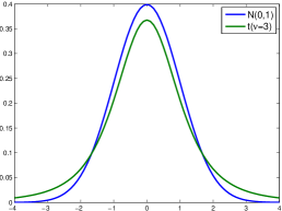
(a) Experiment 1

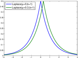
(b) Experiment 2

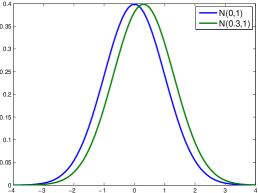
(c) Experiment 3

Figure B.1: An illustration of distribution $P$ vs. $Q$ in our numerical experiments.

In the main text, we presented two numerical experiments, on testing between samples from different distributions $P,Q$. In the first experiment $P=N(0,1)$ and $Q=t_{3}$, so the difference between $P,Q$ was mainly in the tails; in the second, $P=\mathrm{Laplace}(0)$ and $Q=\mathrm{Laplace}(0.3)$, and the difference between $P,Q$ was mainly in the centers of the distributions. The first experiment demonstrated that the power of the higher order KS test generally increased as we increased the polynomial degree $k$, the second demonstrated the opposite, i.e., that its power generally decreased for increasing $k$. Refer back to Figures 5.1 and 5.2 in the main text.

We should note that the first experiment was not carefully crafted in any way; the same performance is seen with a number of similar setups. However, we did have to look carefully to reveal the negative behavior shown in the second experiment. For example, in detecting the difference between mean-shifted standard normals (as opposed to Laplace distributions), the higher order KS tests do not encounter nearly as much difficulty. To demonstrate this, we examine a third experiment here with $P=N(0,1)$ and $Q=N(0.3,1)$. Figure B.1 gives a visual illustration of the distributions across the three experimental setups (the first two considered in the main text, and the third investigated here).

The ROC curves for experiment 3 are given in Figure B.2. The left panel shows that the test for $k=1$ improves on the usual test ($k=0$), even though the difference between the two distributions is mainly near their centers. The right panel shows that the higher order KS tests are competitive with other commonly used nonparametric tests in this setting. The results of this experiment hence suggest that the higher order KS tests provide a utility beyond simply detecting finer tail differences, and the tradeoff induced by varying the polynomial order $k$ is not completely explained as a tradeoff between tail and center sensitivity.

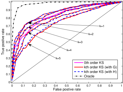
(a) Comparing higher order KS tests

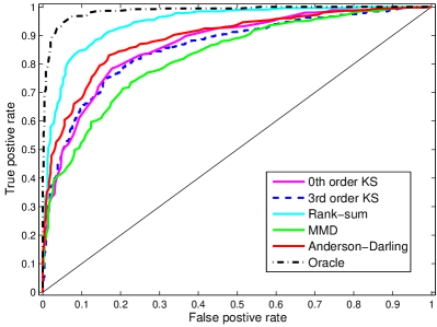
(b) Comparing other tests

Figure B.2: ROC curves for experiment 3, normal vs. shifted normal.

We also study the sample complexity of tests in the three experimental setups. Specifically, over $R=1000$ repetitions, we find the true positive rate associated with a 0.05 false positive rate, as we let $n$ vary over $10,20,50,100,200,\ldots 1000$. The results for this sample complexity sudy are shown in Figures B.3, B.4, and B.5. We see that the higher order KS tests perform quite favorably the first experimental setup, not so favorably in the second, and somewhere in the middle in the third.

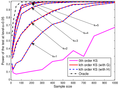
(a) Comparing higher order KS tests

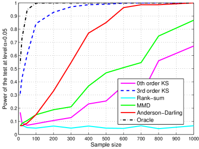
(b) Comparing other tests

Figure B.3: Sample complexities at the level $\alpha=0.05$ for experiment 1, normal vs. t.

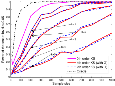
(a) Comparing higher order KS tests

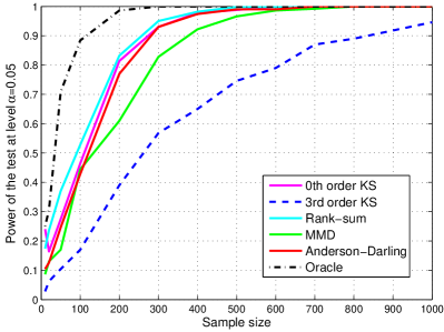
(b) Comparing other tests

Figure B.4: Sample complexities at level $\alpha=0.05$ in experiment 2, Laplace vs. shifted Laplace.

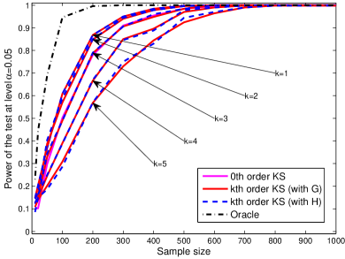
(a) Comparing higher order KS tests

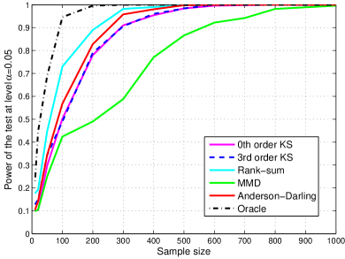
(b) Comparing other tests

Figure B.5: Sample complexities at level $\alpha=0.05$ in experiment 3, normal vs. shifted normal.

References

- Anderson & Darling (1954) Anderson, Theodore and Darling, Donald. A test of goodness of fit. Journal of the American Statistical Association, 49(268):765–769, 1954.
- Barbe (1992) Barbe, Philippe. Limiting distribution of the maximal spacing when the density function admits a positive minimum. Statistics & Probability Letters, 14(1):53–60, 1992.
- Buckheit & Donoho (1995) Buckheit, Jonathan and Donoho, David. Wavelab and reproducible research. Lecture Notes in Statistics, 103:55–81, 1995.
- David & Nagaraja (1970) David, Herbert Aron and Nagaraja, Haikady Navada. Order Statistics. Wiley, Hoboken, 1970.
- de Boor (1978) de Boor, Carl. A Practical Guide to Splines. Springer, New York, 1978.
- Gretton et al. (2012) Gretton, Arthur, Borgwardt, Karsten, Rasch, Malte, Schölkopf, Bernhard, and Smola, Alexander. A kernel two-sample test. Journal of Machine Learning Research, 13:723–773, 2012.
- Kim et al. (2009) Kim, Seung-Jean, Koh, Kwangmoo, Boyd, Stephen, and Gorinevsky, Dimitry. trend filtering. SIAM Review, 51(2):339–360, 2009.
- Mammen & van de Geer (1997) Mammen, Enno and van de Geer, Sara. Locally apadtive regression splines. Annals of Statistics, 25(1):387–413, 1997.
- Nussbaum (1985) Nussbaum, Michael. Spline smoothing in regression models and asymptotic efficiency in . Annals of Statistics, 13(3):984–997, 1985.
- Scholz & Stephens (1987) Scholz, Fritz and Stephens, Michael. K-sample Anderson-Darling tests. Journal of the American Statistical Association, 82(399):918–924, 1987.
- Tibshirani (2014) Tibshirani, Ryan J. Adaptive piecewise polynomial estimation via trend filtering. Annals of Statistics, 42(1):285–323, 2014.
- Wahba (1990) Wahba, Grace. Spline Models for Observational Data. Society for Industrial and Applied Mathematics, Philadelphia, 1990.
- Wilcoxon (1945) Wilcoxon, Frank. Individual comparisons by ranking methods. Biometrics Bulletin, 1(6):80–83, 1945.