Injection of $\kappa$-like Suprathermal Particles into Diffusive Shock Acceleration

Abstract

We consider a phenomenological model for the thermal leakage injection in the diffusive shock acceleration (DSA) process, in which suprathermal protons and electrons near the shock transition zone are assumed to have the so-called $\kappa$-distributions produced by interactions of background thermal particles with pre-existing and/or self-excited plasma/MHD waves or turbulence. The $\kappa$-distribution has a power-law tail, instead of an exponential cutoff, well above the thermal peak momentum. So there are a larger number of potential seed particles with momentum, above that required for participation in the DSA process. As a result, the injection fraction for the $\kappa$-distribution depends on the shock Mach number much less severely compared to that for the Maxwellian distribution. Thus, the existence of $\kappa$-like suprathermal tails at shocks would ease the problem of extremely low injection fractions, especially for electrons and especially at weak shocks such as those found in the intracluster medium. We suggest that the injection fraction for protons ranges $10^{-4}-10^{-3}$ for a $\kappa$-distribution with $10\lesssim\kappa_{p}\lesssim 30$ at quasi-parallel shocks, while the injection fraction for electrons becomes $10^{-6}-10^{-5}$ for a $\kappa$-distribution with $\kappa_{e}\lesssim 2$ at quasi-perpendicular shocks. For such $\kappa$ values the ratio of cosmic ray electrons to protons naturally becomes $K_{e/p}\sim 10^{-3}-10^{-2}$, which is required to explain the observed ratio for Galactic cosmic rays.

1. Introduction

Acceleration of nonthermal particles is ubiquitous at astrophysical collisionless shocks, such as interplanetary shocks in the solar wind, supernova remnant (SNR) shocks in the interstellar medium (ISM) and structure formation shocks in the intracluster medium (ICM) (Blandford & Eichler, 1987; Jones & Ellison, 1991; Ryu et al., 2003). Plasma physical processes operating at collisionless shocks, such as excitation of waves via plasma instabilities and ensuing wave-particle interactions, depend primarily on the shock magnetic field obliquity as well as on the sonic and Alfvénic Mach numbers, $M_{s}$ and $M_{A}$, respectively. Collisionless shocks can be classified into two categories by the obliquity angle, $\Theta_{BN}$, the angle between the upstream mean magnetic field and the shock normal: quasi-parallel ($\Theta_{BN}\lesssim 45^{\circ}$) and quasi-perpendicular ($\Theta_{BN}\gtrsim 45^{\circ}$). Diffusive shock acceleration (DSA) at strong SNR shocks with $M_{s}\sim M_{A}\sim 10-100$ is reasonably well understood, especially for the quasi-parallel regime, and it has been tested via radio-to-$\gamma$-ray observations of nonthermal emissions from accelerated cosmic ray (CR) protons and electrons (see Drury, 1983; Blandford & Eichler, 1987; Hillas, 2005; Reynolds et al., 2012, for reviews). On the contrary, DSA at weak shocks in the ICM ($M_{s}\sim 2-3$, $M_{A}\sim 10$) is rather poorly understood, although its signatures have apparently been observed in a number of radio relic shocks (e.g. van Weeren et al., 2010; Feretti et al., 2012; Kang et al., 2012; Brunetti & Jones, 2014). At the same time, in situ measurements of Earth’s bow shock, or traveling shocks in the interplanetary medium (IPM) with spacecrafts have provided crucial insights and tests for plasma physical processes related with DSA at shocks with moderate Mach numbers ($M_{s}\sim M_{A}\lesssim 10$) (e.g. Shimada et al., 1999; Oka et al., 2006; Zank et al., 2007; Masters et al., 2013).

Table 1 compares characteristic parameters for plasmas in the IPM, ISM (warm phase), and ICM to highlight their similarities and differences. Here the plasma beta $\beta_{p}~{}(=P_{g}/P_{B}\propto n_{H}T/B_{0}^{2}$) is the ratio of the thermal to magnetic pressures, so the magnetic field pressure is dynamically more important in lower beta plasmas. The plasma alpha is defined as the ratio of the electron plasma frequency to cyclotron frequency:

$$\alpha_{p}~{}={\omega_{pe}\over\Omega_{ce}}=\frac{2\pi r_{ge}}{\lambda_{De}}\approx{{\sqrt{m_{e}/m_{p}}\cdot c}\over v_{A}}\propto{\sqrt{n_{e}}\over B_{0}},$$ (1)

where $r_{ge}$ is the electron gyroradius, and $\lambda_{De}$ is the electron Debye length, $v_{A}=B_{0}/\sqrt{4\pi\rho}$ is the Alfvén speed. Plasma wave-particle interactions and ensuing stochastic acceleration are more significant in lower alpha plasmas (e.g. Pryadko & Petrosian, 1997). Among the three kinds of plasmas in Table 1, the ICM with the highest $\beta_{p}$ has dynamically least significant magnetic fields, but, with the smallest $\alpha_{p}$, plasma interactions are expected to be most important there. The last three columns of Table 1 show typical shock speeds, sonic Mach numbers, and Alfvénic Mach numbers for interplanetary shocks near 1 AU, SNR shocks and ICM shocks.

This paper focuses on the injection of suprathermal particles into the DSA process at astrophysical shocks. Since the shock thickness is of the order of the gyroradius of postshock thermal protons, only suprathermal particles (both protons and electrons) with momentum $p\gtrsim p_{\rm inj}\approx(3-4)p_{\rm th,p}$ can re-cross to the shock upstream and participate in the DSA process (e.g. Kang et al., 2002). Here, $p_{\rm th,p}=\sqrt{2m_{p}k_{B}T_{2}}$ is the most probable momentum of thermal protons with postshock temperature $T_{2}$ and $k_{B}$ is the Boltzmann constant. Hereafter, we use the subscripts ‘1’ and ‘2’ to denote the conditions upstream and downstream of shock, respectively. At quasi-parallel shocks, in the so-called thermal injection leakage model, protons leaking out of the postshock thermal pool are assumed to interact with magnetic field fluctuations and become the CR population (e.g. Malkov & Drury, 2001; Kang et al., 2002). In a somewhat different interpretation based on hybrid plasma simulations, protons reflected off the shock transition layer are thought to form a beam of streaming particles, which in turn excite resonant waves that scatter particles into the DSA process (e.g. Quest, 1988; Guo & Giacalone, 2013). At quasi-perpendicular shocks, on the other hand, the self-excitation of waves is ineffective and the injection of suprathermal protons is suppressed significantly (Caprioli & Spitkovsky, 2013), unless there exists pre-existing MHD turbulence in the background plasma (Giacalone, 2005; Zank et al., 2006).

Assuming that downstream electrons and protons have the same kinetic temperature ($T_{e}\approx T_{p}$), for a Maxwellian distribution there will be fewer electrons than protons that will have momenta above the required injection momentum. Thus electrons must be pre-accelerated from the thermal momentum ($p_{\rm th,e}=(m_{e}/m_{p})^{1/2}p_{\rm th,p}$) to the injection momentum ($p_{\rm inj}\approx(130-170)p_{\rm th,e}$) in order to take part in the DSA process. Contrary to the case of protons, which are effectively injected at quasi-parallel shocks, according to in situ observations made by spacecrafts, electrons are known to be accelerated at Earth’s bow shock and interplanetary shocks preferentially in the quasi-perpendicular configuration (e.g. Gosling et al., 1989; Shimada et al., 1999; Simnett et al., 2005; Oka et al., 2006). However, in a recent observation of Saturn’s bow shock by the Cassini spacecraft, the electron injection/acceleration has been detected also in the quasi-parallel geometry at high-Mach, high-beta shocks ($M_{A}\sim 100$ and $\beta_{p}\sim 10$) (Masters et al., 2013). Riquelme & Spitkovsky (2011) suggested that electrons can be injected and accelerated also at quasi-parallel portion of strong shocks such as SNR shocks, because the turbulent magnetic fields excited by the CR streaming instabilities upstream of the shock may have perpendicular components at the corrugated shock surface. So, locally transverse magnetic fields near the shock surface seem essential for the efficient electron injection regardless of the obliquity of the large-scale, mean field.

Non-Maxwellian tails of high energy particles have been widely observed in space and laboratory plasmas (e.g. Vasyliunas, 1968; Hellberg et al., 2000). Such particle distributions can be described by the combination of a Maxwellian-like core and a suprathermal tail of power-law form, which is known as the $\kappa$-distribution. There exists an extensive literature that explains the $\kappa$-distribution from basic physical principles and processes relevant for collisionless, weakly coupled plasmas (e.g. Leubner, 2004; Pierrard & Lazar, 2010). The theoretical justification for the $\kappa$-distribution is beyond the scope of this paper, so readers are referred to those papers. Recently, the existence of $\kappa$-distribution of electrons has been conjectured and examined in order to explain the discrepancies in the measurements of electron temperatures and metallicities in H II regions and planetary nebulae (Nicholls et al., 2012; Mendoza & Bautista, 2014).

The development of suprathermal tails of both proton and electron distributions are two outstanding problems in the theory of collisionless shocks, which involve complex wave-particle interactions such as the excitation of kinetic/MHD waves via plasma instabilities and the stochastic acceleration by plasma turbulence (see Petrosian, 2012; Schure et al., 2012, for recent reviews). For example, stochastic acceleration of thermal electrons by electron-whistler interactions is known to be very efficient in low $\beta_{p}$ and low $\alpha_{p}$ plasmas such as solar flares (Hamilton & Petrosian, 1992). Recently, the pre-heating of electrons and the injection of protons at non-relativistic collisonless shocks have been studied using Particle-in-Cell (PIC) and hybrid plasma simulations for a wide range of parameters (e.g. Amano & Hoshino, 2009; Guo & Giacalone, 2010, 2013; Riquelme & Spitkovsky, 2011; Garaté & Spitkovsky, 2012; Caprioli & Spitkovsky, 2013). In PIC simulations, the Maxwell’s equations for electric and magnetic fields are solved along with the equations of motion for ions and electrons, so full wave-particle interactions can be followed from first principles. In hybrid simulations, only ions are treated kinetically, while electrons are treated as a neutralizing, massless fluid.

Using two and three-dimensional PIC simulations, Riquelme & Spitkovsky (2011) showed that for low Alfvénic Mach numbers ($M_{A}\lesssim 20$), oblique whistler waves can be excited in the foot of quasi-perpendicular shocks (but not at perfectly perpendicular shocks with $\Theta_{Bn}=90^{\circ}$). Electrons are then accelerated via wave-particle interactions with those whistlers, resulting in a power-law suprathermal tail. They found that the suprathermal tail can be represented by the energy spectrum $n_{e}(E)\propto E^{-a}$ with the slope $a=3-4$, which is harder for smaller $M_{A}$ (i.e., larger $v_{A}$ or smaller $\alpha_{p}$). Nonrelativistic electrons streaming away from a shock can resonate only with high frequency whistler waves with right hand helicity, while protons and relativistic electrons (with Lorentz factor $\gamma>m_{p}/m_{e}$) resonate with MHD (Alfvén) waves. So the generation of oblique whistlers is thought to be one of the agents for pre-acceleration of electrons (Shimada et al., 1999). In fact, obliquely propagating whistler waves and high energy electrons are often observed together in the upstream region of quasi-perpendicular interplanetary shocks (e.g. Shimada et al., 1999; Wilson et al., 2009). Recently, Wilson et al. (2012) observed obliquely propagating whistler modes in the precursor of several quasi-perpendicular interplanetary shocks with low Mach numbers (fast mode Mach number $M_{f}\approx 2-5$), simultaneously with perpendicular ion heating and parallel electron acceleration. This observation implies that oblique whistlers could play an important role in the development of a suprathermal halo around the thermal core in the electron velocity distribution at quasi-perpendicular shocks with moderate $M_{A}$.

Using two-dimensional PIC simulations for perpendicular shocks with $M_{A}\sim 45$, Matsumoto et al. (2013) found that several kinetic instabilities (e.g. Buneman, ion-acoustic, ion Weibel) are excited at the leading edge of the shock foot and that electrons can be energized to relativistic energies via the shock surfing mechanism. They suggested that the shock surfacing acceleration can provide the effective pre-heating of electrons at strong SNR shocks with high Alfvénic Mach numbers ($M_{A}\gtrsim 100$).

Because non-relativistic electrons and protons interact with different types of plasma waves and instabilities, they can have suprathermal tails with different properties that depend on plasma and shock parameters, such as $\Theta_{Bn}$, $\alpha_{p}$, $\beta_{p}$, $M_{s}$, and $M_{A}$. So the power-law index of the $\kappa$-distributions for electrons and protons, $\kappa_{e}$ and $\kappa_{p}$, respectively, should depend on these parameters, and they could be significantly different from each other. For example, the electron distributions measured in the IPM can be fitted with the $\kappa$-distributions with $\kappa_{e}\sim 2-5$, while the proton distributions prefer a somewhat larger $\kappa_{p}$ (Pierrard & Lazar, 2010). Using in situ spacecraft data, Neergaard-Parker & Zank (2012) suggested that the proton spectra observed downstream of quasi-parallel interplanetary shocks can be explained by the injection from the upstream (solar-wind) thermal Maxwellian or weak $\kappa$-distribution with $\kappa_{p}\gtrsim 10$. On the other hand, Neergaard-Parker et al. (2014) showed that the upstream suprathermal tail of the $\kappa_{p}=4$ distribution is the best to fit the proton spectra observed downstream of quasi-perpendicular interplanetary shocks. They reasoned that the upstream proton distribution may form a relatively flat $\kappa$-like suprathermal tail due to the particles reflected at the magnetic foot of quasi-perpendicular shocks, while at quasi-parallel shocks the upstream proton distribution remains more-or-less Maxwellian.

In this paper, we consider a phenomenological model for the thermal leakage injection in the DSA process by taking the $\kappa$-distributions as empirical forms for the suprathermal tails of the electron and proton distributions at collisionless shocks. The $\kappa$-distribution is described in Section 2. The injection fraction is estimated in Section 3, followed by a brief summary in Section 4.

2. Basic Models

For the postshock nonrelativistic gas of kinetic temperature $T_{2}$ and particle density $n_{2}$, the Maxwellian momentum distribution is given as

$$f_{\rm M}(p)={n_{2}\over\pi^{1.5}}~{}p_{\rm th}^{-3}~{}\exp\left[-\left({p\over p_{\rm th}}\right)^{2}\right],$$ (2)

where $p_{\rm th}=\sqrt{2mk_{B}T_{2}}$ is the thermal peak momentum and the mass of the particle is $m=m_{e}$ for electrons and $m=m_{p}$ for protons. The distribution function is defined in general as $\int 4\pi p^{2}f(p)dp=n_{2}$. Here we assume that the electron and proton distributions have the same kinetic temperature, so that $p_{\rm th,e}=\sqrt{m_{e}/m_{p}}\cdot p_{\rm th,p}$.

The $\kappa$-distribution can be described as

$$f_{\kappa}(p)={n_{2}\over\pi^{1.5}}~{}p_{\rm th}^{-3}{{\Gamma(\kappa+1)}\over{(\kappa-3/2)^{3/2}\Gamma(\kappa-1/2)}}\left[1+{p^{2}\over{(\kappa-3/2)p_{\rm th}^{2}}}\right]^{-(\kappa+1)},$$ (3)

where $\Gamma(x)$ is the Gamma function (e.g. Pierrard & Lazar, 2010). The $\kappa$-distribution asymptotes to a power-law form, $f_{\kappa}(p)\propto p^{-2(\kappa+1)}$ for $p\gg p_{\rm th}$, which translates into $N(E)\propto E^{-2\kappa}$ for relativistic energies, $E\gtrsim mc^{2}$. For large $\kappa$, it asymptotes to the Maxwellian distribution. For a smaller value of $\kappa$, the $\kappa$-distribution has a flatter, suprathermal, power-law tail, which may result from larger wave-particle interaction rates. Note that for the $\kappa$-distribution in equation (3), the mean energy per particle, $m\langle v^{2}\rangle/2=(2\pi m/n_{2})\int v^{2}f_{\kappa}(p)p^{2}dp$, becomes $(3/2)k_{B}T_{2}$ and the gas pressure becomes $P_{2}=n_{2}k_{B}T_{2}$, providing that particle speeds are nonrelativisitic.

The top panel of Figure 1 compares $f_{\rm M}$ and $f_{\kappa}$ for electrons and protons when $T_{2}=5\times 10^{7}$ K (corresponding to the shock speed of $u_{s}\approx 1.9\times 10^{3}~{}{\rm km~{}s^{-1}}$ in the large $M_{s}$ limit.) Here, the momentum is expressed in units of $m_{e}c$ for both electrons and protons, so the distribution function $f(p)$ is plotted in units of $n_{2}/(m_{e}c)^{3}$. Note that the plotted quantity is $p^{3}f(p)d\ln p=p^{2}f(p)dp\propto n(p)dp$. For smaller values of $\kappa$, the low energy portion of $f_{\kappa}(p)$ also deviates more significantly from $f_{\rm M}(p)$.

For the $\kappa$-distribution, the most probable momentum (or the peak momentum) is related to the Maxwellian peak momentum as $p_{\rm mp}^{2}=p_{\rm th}^{2}\cdot(\kappa-3/2)/\kappa$. So for a smaller $\kappa$, the ratio of $p_{\rm mp}/p_{\rm th}$ becomes smaller. In other words, the peak of $f_{\kappa}(p)$ is shifted to a lower momentum for a smaller $\kappa$, as can be seen in the top panel of Figure 1. To account for this we will suppose a hypothetical case in which the postshock temperature is modified for a $\kappa$-distribution as follows:

$$T_{2}^{\prime}(\kappa)=T_{2}{\kappa\over{(\kappa-3/2)}}.$$ (4)

Then the most probable momentum becomes the same for different $\kappa$’s. The bottom panel of Figure 1 compares the Maxwellian distribution for $T_{2}=5\times 10^{7}$ K and the $\kappa$-distributions with the corresponding $T_{2}^{\prime}(\kappa)$’s. For such $\kappa$-distributions, the distribution of low energy particles with $p\lesssim p_{\rm th}$ remains very similar to the Maxwellian distribution. In that case, low energy particles follow more-or-less the Maxwellian distribution, while higher energy particles above the thermal peak momentum show a power-law tail. This might represent the case in which thermal particles with $p\gtrsim p_{\rm th}$ gain energies via stochastic acceleration by pre-existing and/or self-excited waves in the shock transition layer, resulting in a $\kappa$-like tail and additional plasma heating. Such $\kappa$-distributions with plasma heating could be close to the real particle distributions behind collisionless shocks. So below we will consider two cases: the $T_{2}$ model in which the postshock temperature is same and the $T_{2}^{\prime}$ model in which the postshock temperature depends on $\kappa$ as in equation (4).

3. Injection Fraction

We assume that the distribution function of the particles accelerated by DSA, which we refer to as cosmic rays (CRs), at the position of the shock has the test-particle power-law spectrum for $p\geq p_{\rm inj}\equiv Q_{\rm inj}\cdot p_{\rm th,p}$,

$$f_{\rm CR}(p)=f(p_{\rm inj})\cdot\left({p\over p_{\rm inj}}\right)^{-q},$$ (5)

where the power-law slope is given as

$$q={{3(u_{1}-v_{A,1})}\over u_{1}-v_{A,1}-u_{2}}.$$ (6)

Here $u_{1}$ and $u_{2}$ are the upstream and downstream flow speeds, respectively, in the shock rest frame, and $v_{A,1}=B_{1}/\sqrt{4\pi\rho_{1}}$ is the upstream Alfvén speed. This expression takes account of the drift of the Alfvén waves excited by streaming instabilities in the shock precursor (e.g., Kang, 2011, 2012). If $v_{A,1}=0$, the power-law slope becomes $q=4$ for $M_{s}\gg 1$ and $q=4.5$ for $M_{s}=3$.

Note that in our phenomenological model, we assume the $\kappa$-distribution extends only to $p=p_{\rm inj}$, above which the DSA power-law in equation (5) sets in. In Figure 1 the vertical dotted lines show the range of $p_{\rm inj}=(3.5-4)\ p_{\rm th,p}$, above which the particles can participate the DSA process. With $\kappa_{p}=30$ for protons, $\kappa_{e}=2$ for electrons, and $p_{\rm inj}=4p_{\rm th,p}$, for example, the ratio of $f_{e}(p_{\rm inj})/f_{p}(p_{\rm inj})\approx 10^{-2.6}$ for the $T_{2}$ model, while $f_{e}(p_{\rm inj})/f_{p}(p_{\rm inj})\approx 10^{-1.9}$ for the $T_{2}^{\prime}$ model.

The parameter $Q_{\rm inj}$ determines the CR injection fraction, $\xi\equiv{n_{CR}/n_{2}}$ as follows. In the case of the Maxwellian distribution the fraction is

$$\xi_{\rm M}={4\over\sqrt{\pi}}{{Q_{\rm inj}^{3}}\over{(q-3)}}\cdot\exp(-Q_{\rm inj}^{2}),$$ (7)

while in the case of the $\kappa$-distribution it is

$$\xi_{\kappa}={4\over\sqrt{\pi}}{{Q_{\rm inj}^{3}}\over{(q-3)}}\cdot{{\Gamma(\kappa+1)}\over{(\kappa-3/2)^{3/2}\Gamma(\kappa-1/2)}}\left[1+{Q_{\rm inj}^{2}\over{(\kappa-3/2)}}\right]^{-(\kappa+1)}.$$ (8)

Note that both forms of the injection fraction are independent of the postshock temperature $T_{2}$, but dependent on $Q_{\rm inj}$ and the shock Mach number, through the slope $q(M_{s})$.

For the Maxwellian distribution, $\xi_{\rm M}$ decreases exponentially with the parameter $Q_{\rm inj}$, which in general depends on the shock Mach number as well as on the obliquity. Since the injection process should depend on the level of pre-existing and self-excited plasma/MHD waves, $Q_{\rm inj}$ is expected to increase with $\Theta_{Bn}$. For example, in a model adopted for quasi-parallel shocks (e.g. Kang & Ryu, 2010),

$$Q_{\rm inj}\approx\chi{{m_{p}u_{2}}\over{p_{\rm th,p}}}=\chi\sqrt{{\gamma\over{2\mu}}}{u_{2}\over c_{s,2}}=\chi\sqrt{{\gamma\over{2\mu}}}\left[{{(\gamma-1)M_{s}^{2}+2}\over{2\gamma M_{s}^{2}-(\gamma-1)}}\right]^{1/2},$$ (9)

where $\chi\approx 5.8-6.6$, $\gamma$ is the gas adiabatic index, and $\mu$ is the mean molecular weight for the postshock gas. For $\gamma=5/3$ and $\mu=0.6$, this parameter approaches to $Q_{\rm inj}\approx 3-4$ for large $M_{s}$, depending on the level of MHD turbulence, and it increases as $M_{s}$ decreases (see Figure 1 of Kang & Ryu (2010)). Using hybrid plasma simulations, Caprioli & Spitkovsky (2013) suggested $Q_{\rm inj}=3-4$ at quasi-parallel shocks with $M_{s}\approx M_{A}\approx 20$, leading to the injection fraction of $\xi_{p}\approx 10^{-4}-10^{-3}$ for protons.

For highly oblique and perpendicular shocks, the situation is more complex and the modeling of $Q_{\rm inj}$ becomes difficult, partly because MHD waves are not self-excited effectively and partly because the perpendicular diffusion is not well understood (e.g. Neergaard-Parker et al., 2014). So the injection process at quasi-perpendicular shocks depends on the pre-existing MHD turbulence in the upstream medium as well as the angle $\Theta_{Bn}$. For example, Zank et al. (2006) showed that in the case of interplanetary shocks in the solar wind located near 1AU from the sun, the injection energy is similar for $\Theta_{Bn}=0^{\circ}$ and $90^{\circ}$, but it peaks at highly oblique shocks with $\Theta_{Bn}\sim 60-80^{\circ}$. So $Q_{\rm inj}$ would increase with $\Theta_{Bn}$, but decrease as $\Theta_{Bn}\rightarrow 90^{\circ}$. The same kind of trend may apply for cluster shocks, but again the details will depend on the MHD turbulence in the ICM. Here we will consider a range of values, $3\leq Q_{\rm inj}\leq 5$. For the $\kappa$-distribution, $\xi_{\kappa}$ also decreases with $Q_{\rm inj}$ but more slowly than $\xi_{M}$ does. This means that the dependence of injection fraction on the shock sonic Mach number would be weaker in the case of the $\kappa$-distribution.

Figure 2 shows the energy spectrum of protons for the two (i.e., $T_{2}$ and $T_{2}^{\prime}$) models shown in Figure 1. Here the energy spectrum is calculated as $n_{p}(E)=4\pi p^{2}f(p)({dp}/{dE})$, where the kinetic energy is $E=\sqrt{p^{2}c^{2}+m_{p}^{2}c^{4}}-m_{p}c^{2}$ and the distribution function $f(p)$ is given in equations (2) or (3). The filled and open circles mark the spectrum at the energies corresponding to $3.5\ p_{\rm th,p}$ and $4\ p_{\rm th,p}$ for the Maxwellian distribution and the $\kappa$-distributions with $\kappa_{p}=10$ and 30. This shows that the injection efficiency for CR protons would be enhanced in the $\kappa$-distributions, compared to the Maxwellian distribution, by a factor of $\xi_{\kappa_{p}=10}/\xi_{\rm M}\sim 100-300$ and $\xi_{\kappa_{p}=30}/\xi_{\rm M}\sim 10-20$.

There are reasons why the cases of $\kappa_{p}=10-30$ are shown here. It has been suggested that the upstream suprathermal populations can be represented by the $\kappa$-distribution with $\kappa_{p}\approx 4$ at quasi-perpendicular IPM shocks (Neergaard-Parker et al., 2014) and $\kappa_{p}\gtrsim 10$ at quasi-parallel IPM shocks (Neergaard-Parker & Zank, 2012). However, the proton injection at quasi-parallel shocks is much more efficient than that at quasi-perpendicular shocks, because the injection energy is much higher at highly oblique shocks (e.g. Zank et al., 2006). Moreover, Caprioli & Spitkovsky (2013) showed that the proton injection at quasi-parallel shocks can be modeled properly with the thermal leakage injection from the Maxwellian distribution at $p_{\rm inj}\approx(3-4)p_{\rm th,p}$. They also showed that a harder suprathermal population forms at larger $\Theta_{BN}$, which is consistent with the observations at IPM shocks. But the power-law CR spectrum does not develop at (almost) perpendicular shocks due to lack of self-excited waves in their hybrid simulations.

As shown in Figure 1 the electron distribution needs a substantially more enhanced suprathermal tail, for example, the one in the $\kappa$-distribution with $\kappa_{e}\sim 2$, in order to achieve the electron-to-proton ratio $K_{e/p}\sim 10^{-3}-10^{-2}$ with the thermal leakage injection model. Figure 3 shows the energy spectrum of electrons for the two models shown in Figure 1. Here the energy spectrum for electrons is calculated as $n_{e}(\Gamma_{e}-1)=4\pi p^{2}f(p)({dp}/{d\Gamma_{e}})$, where the Lorentz factor is $\Gamma_{e}=\sqrt{1+(p/m_{e}c)^{2}}$. The filled and open circles mark the spectrum at the energies corresponding to $p_{\rm inj}=(3.5-4)\ p_{\rm th,p}$ for the $\kappa$-distributions with $\kappa_{e}=1.6,2.0$, and 2.5. Note that the $\kappa$-distribution is defined for $\kappa>3/2$. In the PIC simulations of quasi-perpendicular shocks by Riquelme & Spitkovsky (2011), the power-law slope of $n_{e}(E)$ at $\Gamma_{e}\sim 10-100$ ranges $2.7<a<4$ for $3.5\leq M_{A}\leq 14$, where $m_{p}/m_{e}=1600$ was adopted (see their Figure 12). This would translate roughly into $\kappa_{e}\lesssim 2$, which is consistent with the observations at quasi-perpendicular IPM shocks (Pierrard & Lazar, 2010).

If the suprathermal tails of electrons and protons can be described by the $\kappa$-distributions with $\kappa_{e}$ and $\kappa_{p}$, respectively, for $p\leq p_{\rm inj}$, and if both CR electrons and protons have simple power-laws given in equation (5) for $p>p_{\rm inj}$, then the injection fractions, $\xi_{p}$ and $\xi_{e}$, for $\kappa$-distributions can be estimated by equation (8). Figure 4 compares the injection fractions, $\xi_{p}$ and $\xi_{e}$, for the two models shown in Figures 1-3. Note that the slope $q$ depends on $M_{s}$, so $\xi(q-3)$ is plotted instead of just $\xi$. Now the ratio of CR electron to proton numbers can be calculated as

$$K_{e/p}(Q_{\rm inj},\kappa_{e},\kappa_{p})\equiv{{\xi_{e}(Q_{\rm inj},\kappa_{e})}\over{\xi_{p}(Q_{\rm inj},\kappa_{p})}}={{f_{e}(p_{\rm inj},\kappa_{e})}\over{f_{p}(p_{\rm inj},\kappa_{p})}}.$$ (10)

In the $\kappa$-distribution of protons with $\kappa_{p}=30$ (dot-dashed line), for example, $\xi_{p}$ decrease from $10^{-3}$ to $10^{-4}$ when $Q_{\rm inj}$ increase from 3.5 to 4. We note that for $\kappa_{p}\lesssim 10$ or for $Q_{\rm inj}\lesssim 3.5$, the proton injection fraction would be too high (i.e., $\xi_{p}>10^{-3}$) to be consistent with commonly-accepted DSA modelings of observed shocks such as SNRs. The parameter $Q_{\rm inj}$ would in general increase for a smaller $M_{s}$ as illustrated in equation (9). The dependence of the injection fraction on $M_{s}$ becomes weaker for the $\kappa$-distribution than for the Maxwellian distribution. As a result, the suppression of the CR injection fraction at weak shocks will be less severe if the $\kappa$-distribution is considered.

For electrons, the injection fraction would be too small if they were to be injected by way of thermal leakage from the Maxwellian distribution. So that case is not included in Figure 4. The expected electron injection would be $\xi_{e}\sim 10^{-6}-10^{-5}$, if one takes $K_{e/p}\sim 10^{-3}-10^{-2}$ and $\xi_{p}\sim 10^{-4}-10^{-3}$. Then, the suprathermal tails of the $\kappa$-distributions with $\kappa_{e}\lesssim 2$ would be necessary. For electron distributions with such flat suprathermal tails, the injection fraction would not be significantly suppressed even at weak shocks.

Turbulent waves excited in the shock precursor/foot should decay away from the shock (both upstream and downstream), as seen in the interplanetary shocks (Wilson et al., 2012) and the PIC simulations (Riquelme & Spitkovsky, 2011). Thus it is possible the $\kappa$-like suprathermal electron populations exist only in a narrow region around the shock, and in any case the differences from Maxwellian form that we discuss here are too limited to produce easily observable signatures such as clearly nonthermal hard X-ray bremsstrahlung.

During the very early stage of SNR expansion with $u_{s}>10^{4}~{}{\rm km~{}s^{-1}}$, the postshock electrons should be described by the relativistic Maxwellian distribution with a relatively slow exponential cutoff of $\exp(-\Gamma_{e}m_{e}c^{2}/k_{B}T)$ instead of equation (2). However, injection from relativistic electron plasmas at collisionless shocks could involve much more complex plasma processes and lie beyond the scope of this study.

4. Summary

In the so-called thermal leakage injection model for DSA, the injection fraction depends on the number of suprathermal particles near the injection momentum, $p_{\rm inj}=Q_{\rm inj}p_{\rm th,p}$, above which the particles can participate in the DSA process (e.g. Kang et al., 2002). The parameter $Q_{\rm inj}$ should be larger for larger oblique angle, $\Theta_{Bn}$, and for smaller sonic Mach number, $M_{s}$, leading to a smaller injection fraction. Moreover, it should depend on the level of magnetic field turbulence, both pre-existing and self-excited, which in turn depends on the plasma parameters such as $\beta_{p}$ and $\alpha_{p}$ as well as the power-spectrum of MHD turbulence. Since the detailed plasma processes related with the injection process are not fully understood, here we consider a feasible range, $3\leq Q_{\rm inj}\leq 5$.

Assuming that suprathermal particles, both protons and electrons, follow the $\kappa$-distribution with a wide range of the power-law index, $\kappa_{p}$ and $\kappa_{e}$, we have calculated the injection fractions for protons and electrons. A $\kappa$-type distribution or distribution consisting of a quasi-thermal plus a nonthermal tail, with a short dynamic range as the one needed here, is expected in a variety of models for acceleration of nonrelativistic thermal particles (see e.g. Petrosian & East (2008) for acceleration in ICM or Petrosian & Lui (2004) for acceleration in Solar flares). The fact that efficient accelerations of electrons and protons require $\kappa$-type distributions with different values of $\kappa$ suggests that they are produced by interactions with different types of waves; e.g., Alfven waves for protons and whistler waves for electrons. We show that $\kappa_{p}\sim 10-30$ leads to the injection fraction of $\xi_{p}\sim 10^{-4}-10^{-3}$ for protons at quasi-parallel shocks, while $\kappa_{e}\lesssim 2$ leads to the injection fraction of $\xi_{e}\sim 10^{-6}-10^{-5}$ for electrons at quasi-perpendicular shocks. The proton injection is much less efficient at quasi-perpendicular shocks, compared to quasi-parallel shocks, because MHD waves are not efficiently self-excited (Zank et al., 2006; Caprioli & Spitkovsky, 2013). For electrons, a relatively flat $\kappa$-distribution may form due to obliquely propagating whistlers at quasi-perpendicular shocks with moderate Mach numbers ($M_{A}\lesssim 20$), and $\kappa_{e}$ is expected to decrease for a smaller $M_{A}$ (i.e. smaller $\alpha_{p}$ or stronger magnetization) (Riquelme & Spitkovsky, 2011). We note that these $\kappa$-like suprathermal populations are expected to exist only in a narrow region around the shock, since they should be produced via plasma/MHD interactions with various waves, which could be excited in the shock precursor and then decay downstream.

In addition, we point out that acceleration (to high CR energies) is less sensitive to shock and plasma parameters for a $\kappa$-distribution than the Maxwellian distribution. So, the existence of $\kappa$-like suprathermal tails in the electron distribution would alleviate the problem of extremely low injection fractions for weak quasi-perpendicular shocks such as those widely thought to power radio relics found in the outskirts of galaxy clusters (Kang et al., 2012; Pinzke et al., 2013; Brunetti & Jones, 2014).

Finally, we mention that electrons are not likely to be accelerated at weak quasi-parallel shocks, according to in situ measurements of interplanetary shocks (e.g. Oka et al., 2006) and PIC simulations (e.g. Riquelme & Spitkovsky, 2011). At strong quasi-parallel shocks, on the other hand, Riquelme & Spitkovsky (2011) suggested that electrons could be injected efficiently through locally perpendicular portions of the shock surface, since turbulent magnetic fields are excited and amplified by CR protons streaming ahead of the shock. Thus the magnetic field obliquity, both global and local to the shock surface, and magnetic field amplification via wave-particle interactions are among the key players that govern the CR injection at collisionless shocks and need to be further studied by plasma simulations.

Table 1.  Characteristic Plasma Parameters^a

	$n_{H}$	$T$	$B$	$c_{s}$	$v_{A}$	$\beta_{p}$	$\alpha_{p}$	$u_{s}$	$M_{s}$	$M_{A}$
	$(\rm cm^{-3})$	(K)	($\mu$G)	(${\rm km~{}s^{-1}}$)	(${\rm km~{}s^{-1}}$)	($P_{g}/P_{B}$)	($\omega_{pe}/\Omega_{e}$)	(${\rm km~{}s^{-1}}$)
IPM	5	$10^{5}$	50	50	40	1.6	140	$5\times 10^{2}$	10	13
ISM	0.1	$10^{4}$	5	15	30	0.3	200	$3\times 10^{3}$	200	100
ICM	$10^{-4}$	$5\times 10^{7}$	1	$10^{3}$	180	40	30	$2\times 10^{3}$	2	11

^aIPM=interplanetary medium, ISM=interstellar medium, ICM=intracluster medium

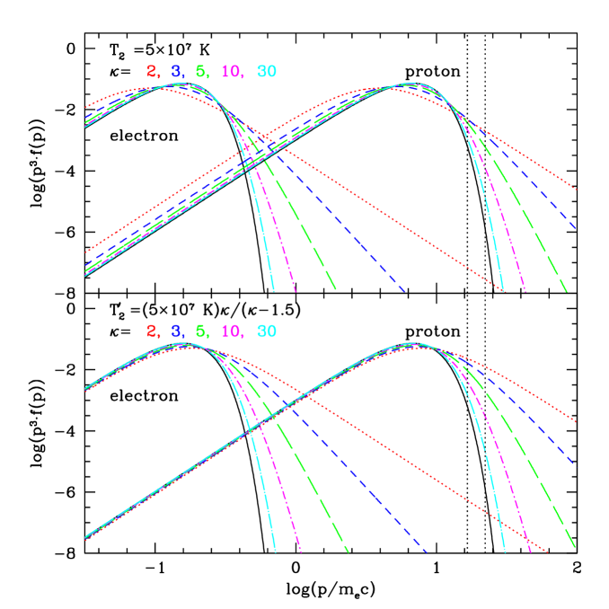
Figure 1.— Momentum distribution, $p^{3}f(p)$, of electrons and protons for kinetic temperature $T_{2}=5\times 10^{7}$ K (top) and $T_{2}^{\prime}$ given equation (4) (bottom). The momentum is expressed in units of $m_{e}c$ for both electrons and protons, and the distribution function $f(p)$ is plotted in units of $n_{2}/(m_{e}c)^{3}$. The Maxwellian distributions are shown in (black) solid lines, while the $\kappa$-distributions are shown in (red) dotted, (blue) dashed, (green) long dashed, (magenta) dot-dashed, and (cyan) dot-long dashed lines for $\kappa=$ 2, 3, 5, 10, and 30, respectively. The vertical lines indicate the range of the injection momentum of $p_{\rm inj}=(3.5-4)\ p_{\rm th,p}$, above which particles can be injected into the DSA process.

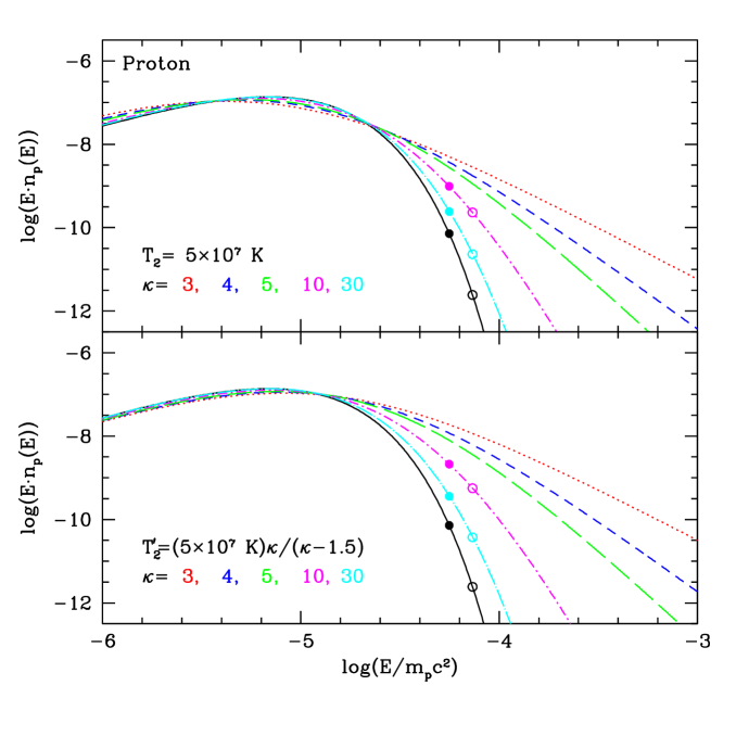
Figure 2.— Kinetic energy spectrum for protons, $E\cdot n_{p}(E)$, for kinetic temperature $T_{2}=5\times 10^{7}$ K (top) and $T_{2}^{\prime}$ given equation (4) (bottom). The kinetic energy, $E$, is expressed in units of $m_{p}^{2}c$ and the energy spectrum, $n_{p}(E)$, is plotted in units of $n_{2}/(m_{p}c^{2})$. The Maxwellian distributions are shown in (black) solid lines, while the $\kappa$-distributions are shown in (red) dotted, (blue) dashed, (green) long dashed, (magenta) dot-dashed, and (cyan) dot-long dashed lines for $\kappa=$ 3, 4, 5, 10, and 30, respectively. Three filled and open circles indicate $3.5\ p_{\rm th,p}$ and $4\ p_{\rm th,p}$, respectively.

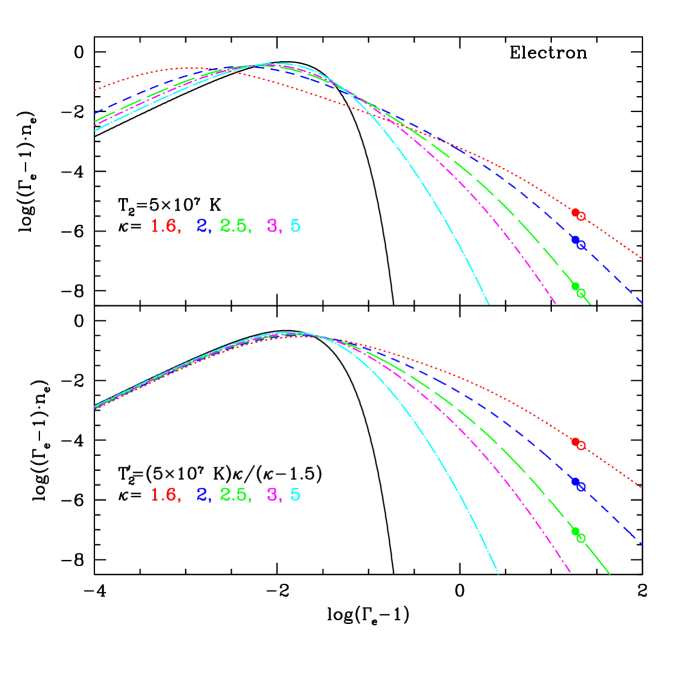
Figure 3.— Energy spectrum for electrons, $(\Gamma_{e}-1)\cdot n_{e}(\Gamma_{e})$, for kinetic temperature $T_{2}=5\times 10^{7}$ K (top) and $T_{2}^{\prime}$ given equation (4) (bottom), where $\Gamma_{e}$ is the Lorentz factor. The Maxwellian distributions are shown in (black) solid lines, while the $\kappa$-distributions are shown in (red) dotted, (blue) dashed, (green) long dashed, (magenta) dot-dashed, and (cyan) dot-long dashed lines for $\kappa=$ 1.6, 2, 2.5, 3, and 5 respectively. Three filled and open circles indicate $3.5\ p_{\rm th,p}$ and $4\ p_{\rm th,p}$, respectively.

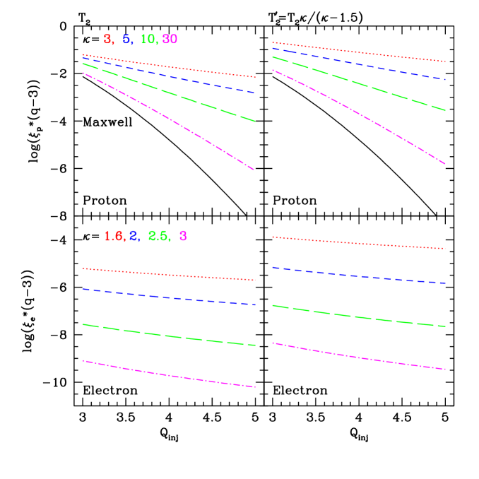
Figure 4.— Fraction of injected CR protons, $\xi_{p}\cdot(q-3)$, and electrons, $\xi_{e}\cdot(q-3)$, given in equations (7) $-$ (8) as a function $Q_{\rm inj}=p_{\rm inj}/p_{\rm th,p}$ for the $T_{2}$ (left panels) and $T_{2}^{\prime}$ (right panels) model. The CR spectrum is assumed to be a power-law given in equation (5) for $p\geq p_{\rm inj}$. For protons (top panels) the Maxwellian distributions are shown in (black) solid lines, while the $\kappa_{p}$-distributions are shown in (red) dotted, (blue) dashed, (green) long dashed, and (magenta) dot-dashed lines for $\kappa=$ 3, 5, 10, and 30, respectively. For electrons (bottom panels) only the $\kappa$-distributions are shown in (red) dotted, (blue) dashed, (green) long dashed, and (magenta) dot-dashed lines for $\kappa=$ 1.6, 2, 2.5, and 3, respectively.

References

- Amano & Hoshino (2009) Amano, T., & Hoshino, M. 2009, ApJ, 690, 244
- Bell (1978) Bell, A. R. 1978, MNRAS, 182, 147
- Blandford & Eichler (1987) Blandford, R. D., & Eichler, D. 1987, Phys. Rept., 154, 1
- Brunetti & Jones (2014) Brunetti, G., & Jones, T. W. 2014, Int. J. of Modern Physics D. 23, 000
- Caprioli & Spitkovsky (2013) Caprioli, D. & Spitkovsky, A. 2013, ApJ, 765, L20
- Drury (1983) Drury, L. O’C. 1983, Rept. Prog. Phys., 46, 973
- Feretti et al. (2012) Feretti, L., Giovannini, G., Govoni, F., & Murgia, M. 2012, A&A Rev, 20, 54
- Garaté & Spitkovsky (2012) Gargaté L. & Spitkovsky, A. 2012, ApJ, 744, 67
- Giacalone (2005) Giacalone, J. 2005, ApJ, 628, L37
- Gosling et al. (1989) Gosling, J. T., Thomsen, M. F.,& Bame, S. J. 1989, J. Geophys. Res., 94, 10011
- Guo & Giacalone (2010) Guo, F., & Giacalone, J. 2010, ApJ, 715, 406
- Guo & Giacalone (2013) Guo, F., & Giacalone, J. 2013, ApJ, 773, 158
- Hamilton & Petrosian (1992) Hamilton, R. J., & Petrosian, V. 1992, ApJ, 398, 350
- Hellberg et al. (2000) Hellberg, M. A., Mace, R. L., Armstrong, R. J., & Karlstad, G. 2000, J. Plasma Phys. 64, 433
- Hillas (2005) Hillas, A. M., 2005, Journal of Physics G, 31, R95
- Jones & Ellison (1991) Jones, F.C., & Ellison, D.C. 1991,Space Sci. Rev., 58, 259
- Kang (2011) Kang, H. 2011, J. Korean Astron. Soc., 44, 1
- Kang (2012) Kang, H. 2012, J. Korean Astron. Soc., 45, 127
- Kang et al. (2002) Kang, H., Jones, T. W., & Gieseler, U.D.J. 2002, ApJ, 579, 337
- Kang & Ryu (2010) Kang, H., & Ryu, D. 2010, ApJ, 721, 886
- Kang et al. (2012) Kang, H., Ryu, D., & Jones, T. W. 2012, ApJ, 756, 97
- Leubner (2004) Leubner, M.P. 2004, Physics of Plasmas, 11, 1308
- Malkov & Drury (2001) Malkov, M. A., & Drury, L.O’C. 2001, Rep. Progr. Phys., 64, 429
- Masters et al. (2013) Masters, A., Stawarz, L., Fujimoto, M., et al. 2013, Nat. Phys., 9, 164
- Matsumoto et al. (2013) Matsumoto, Y., Amano, T., & Hoshino, M. 2013, Phys. Rev. Lett., 111, 215003
- Mendoza & Bautista (2014) Mendoza, C. & Bautista, M. A. 2014, ApJ, 785, 91
- Neergaard-Parker & Zank (2012) Neergaard-Parker, L., & Zank, G.P. 2012, ApJ, 757, 97
- Neergaard-Parker et al. (2014) Neergaard-Parker, L., Zank, G.P., & Hu, Q. 2014, ApJ, 782, 52
- Nicholls et al. (2012) Nicholls, D.C., Dopita, M.A., & Sutherland, R. S. 2012, ApJ, 752, 148
- Oka et al. (2006) Oka, M., Terasawa, T., Seki, Y., et al. 2006, Geophys. Res. Lett., 33, L24104
- Petrosian (2012) Petrosian, V. 2012, Space Sci. Rev., 173, 535
- Petrosian & East (2008) Petrosian, V., & East, W. E. 2008, ApJ, 682, 175
- Petrosian & Lui (2004) Petrosian, V., & Lui, S. 2004, ApJ, 610, 550
- Pierrard & Lazar (2010) Pierrard, V., & Lazar, M. 2010, Sol. Phys., 265, 153
- Pinzke et al. (2013) Pinzke, A., Oh, S. P., & Pfrommer, C. 2013 MNRAS, 435, 1061
- Pryadko & Petrosian (1997) Pryadko, J. M., & Petrosian, V. 1997, ApJ, 482, 774
- Quest (1988) Quest, K.B. 1988, J. Geophys. Res., 93, 9649
- Reynolds et al. (2012) Reynolds, S. P., Gaensler, B. M., & Bocchino, F. 2012, Space Sci. Rev., 166, 231
- Riquelme & Spitkovsky (2011) Riquelme, M. A., & Spitkovsky, A. 2011, ApJ, 733, 63
- Ryu et al. (2003) Ryu, D., Kang, H., Hallman, E., & Jones, T. W. 2003, ApJ, 593, 599
- Schure et al. (2012) Schure, K. M., Bell, A. R, Drury, L. O’C., &. Bykov, A. M. 2012, Space Sci. Rev., 173, 491
- Shimada et al. (1999) Shimada, N., Terasawa, T., Hoshino, M., et al. 1999, Ap&SS, 264, 481
- Simnett et al. (2005) Simnett, G.M., Sakai, J.-I., & Forsyth, R.J. 2005, A&A, 440, 759
- Vasyliunas (1968) Vasyliunas, V. M. 1968, J. Geophys. Res., 73, 2839
- van Weeren et al. (2010) van Weeren, R., Röttgering, H. J. A., Brüggen, M., & Hoeft, M. 2010, Science, 330, 347
- Wilson et al. (2009) Wilson, L. B., III, Cattell, C. A., Kellogg, P. J. et al. 2009, J. Geophys. Res., 114, A10106
- Wilson et al. (2012) Wilson, L. B., III, Koval, A., Szabo, A. et al. 2012, Geophys. Res. Lett., 39, L08109
- Zank et al. (2006) Zank, G. P., Li, G., Florinski, V., et al. 2006, J. Geophys. Res., 111, A06108
- Zank et al. (2007) Zank, G.P, Li, G., & Verkhoglyadova, O. 2007, Space Sci. Rev., 130, 255