Percolation on sparse networks
Abstract
We study percolation on networks, which is used as a model of the resilience of networked systems such as the Internet to attack or failure and as a simple model of the spread of disease over human contact networks. We reformulate percolation as a message passing process and demonstrate how the resulting equations can be used to calculate, among other things, the size of the percolating cluster and the average cluster size. The calculations are exact for sparse networks when the number of short loops in the network is small, but even on networks with many short loops we find them to be highly accurate when compared with direct numerical simulations. By considering the fixed points of the message passing process, we also show that the percolation threshold on a network with few loops is given by the inverse of the leading eigenvalue of the so-called non-backtracking matrix.
Percolation, the random occupation of sites or bonds on a lattice or network with independent probability , is one of the best-studied processes in statistical physics. It is used as a model of porous media Machta91 ; MG95 , granular and composite materials OT98 ; Tobochnik99 ; BFD92 ; BG92 , resistor networks ARC85 , forest fires Henley93 , and many other systems of scientific interest. In this paper we study the bond (or edge) percolation process on general networks or graphs, which is used to model the spread of disease Grassberger83 ; Newman02c and network robustness CEBH00 ; CNSW00 ; Holme02a in social and technological networks, among other things. Although percolation has been studied extensively on simple model networks such as random graphs CEBH00 ; CNSW00 ; GDM08 ; Janson09 , there are few analytic results for real-world networks, whose structure is typically more complicated. We show that percolation properties of networks can be calculated using a message passing technique, leading to a range of new results. In particular, we derive equations for the size of the percolating cluster and the average size of non-percolating clusters, which can be solved rapidly by numerical iteration given the structure of a network and the value of . By expanding the message passing equations about the critical point we also derive an expression for the position of the percolation threshold, showing that the critical value of is given by the inverse of the leading eigenvalue of the so-called non-backtracking matrix Hashimoto89 ; Krzakala13 , an edge-based matrix representation of network structure that has found recent use in studies of community detection and centrality in networks Krzakala13 ; MZN14 . The quantities we calculate are averages over all possible realizations of the randomness inherent in the percolation process, rather than over a single realization, obviating the need for a separate average over realizations as is typically required in direct numerical simulations.
We focus in particular on sparse networks, those for which only a small fraction of possible edges are present, which includes most real-world networks. Our results are exact for large, sparse networks that contain a vanishing density of short loops, but even for networks that do contain loops, as most real-world networks do, we find the cluster size calculations to be highly accurate and the threshold calculations can be shown to give a lower bound on the true percolation threshold.
Consider, then, a bond percolation process on an arbitrary undirected network of nodes and edges. Edges are occupied uniformly at random with probability or unoccupied with probability . The primary entities of interest are the percolation clusters, sets of nodes connected by occupied edges. Since percolation is a random process, one cannot know with certainty the identity of the clusters ahead of time, but some things are known. In general there will (with high probability) be at most one percolating cluster, a cluster that fills a non-vanishing fraction of the network in the limit of large , plus an extensive number of small clusters of finite average size. The percolating cluster appears only for sufficiently large values of and the percolation threshold is the value above which it appears; below there are only small clusters.
Define to be the probability that node belongs to a small cluster of exactly nodes, averaged over many realizations of the random percolation process. If the network is a perfect tree—if it contains no loops—then the size of the cluster is equal to one (for node itself) plus the sum of the numbers of nodes reachable along each edge attached to , which is zero if the edge is unoccupied or nonzero otherwise. If, on the other hand, there are loops in the network then this calculation will not, in general, give the exact value of , since it may be possible to reach the same node along two different occupied edges, which leads to overcounting. If the network is sparse, however, and locally tree-like, meaning that in the limit of large network size an arbitrarily large neighborhood around any node takes the form of a tree (and hence contains no loops), then our calculation gives a good approximation, which becomes exact in the limit.
Working in the large limit then and assuming the network to be locally tree-like, the probability is equal to the probability that the numbers of nodes reachable along each edge from add up to , which we can write as
| (1) |
where is the probability that exactly nodes are reachable along the edge connecting and , is the set of immediate network neighbors of node , and is the Kronecker delta.
We now introduce a probability generating function , whose value is given by
| (2) |
which can be conveniently written as
| (3) |
where is the generating function for .
To calculate , we note that is zero if the edge between and is unoccupied (which happens with probability ) and nonzero otherwise (probability ), which means that , and for
| (4) |
where the notation denotes the set of neighbors of excluding . Substituting this expression into the definition of above, we then find that
| (5) |
This self-consistent equation for the generating function suggests a message-passing algorithm: for any value of one guesses (for instance at random) an initial set of values for the and feeds them into the right-hand side of Eq. (5), giving a new set of values on the left. Repeating this process to convergence gives a solution for the generating functions, which can then be substituted into Eq. (3) to give the generating function for the cluster probabilities , from which we can recover the probabilities themselves by differentiating.
As an example application of this method, note that, since is the probability that belongs to a small (non-percolating) cluster of size , the probability that it belongs to a small cluster of any size is and the probability that it belongs to the percolating cluster is one minus this. Then the expected fraction of the network occupied by the entire percolating cluster is given by the average over all nodes:
| (6) |
Setting in Eq. (5) we have
| (7) |
and the solution of this equation, for instance by iteration from a random initial guess, allows us to calculate the size of the percolating cluster Rivoire05 . We give illustrative applications to several networks below.
As another example, consider the case were vertex does not belong to the percolating cluster. Then the expected size of the cluster it does belong to is given by
| (8) |
and, differentiating Eq. (5), we have
| (9) |
By iterating both Eq. (7) and Eq. (9) from random initial values and substituting the results into Eq. (8) we can calculate the expected cluster size. Or we can average over all vertices to calculate the network-wide average size of a non-percolating cluster.
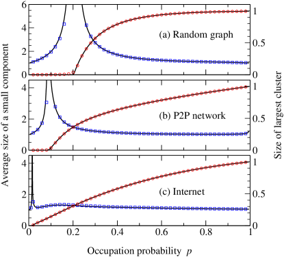
Figure 1 shows results from the application of these techniques to the calculation of cluster sizes for three networks: a computer-generated network which is genuinely tree-like (so the method should work well), and two real-world networks for which percolation could be useful as a model of resilience—a network representation of the Internet at the level of autonomous systems and a peer-to-peer file sharing network. Also shown on the figure are results from direct numerical simulations of percolation on the same networks. As the figure shows, the message passing and numerical results are in excellent agreement, not only for the computer-generated example but also for the two real-world networks, even though the latter are not tree-like. Both the size of the percolating cluster and the mean size of the small clusters are given accurately by the message passing method.
One might ask what the virtue of the message passing method is if one can perform direct percolation simulations of the kind used in Fig. 1. There are two answers to this question. First, simulation algorithms calculate cluster sizes for only a single realization of the randomness inherent in the percolation process. To get accurate results the simulation must be repeated over many realizations, but this can take a significant amount of time and even then the final results still contain statistical errors. The message passing method on the other hand returns the cluster size distribution over all realizations of the randomness in a single calculation.
Second, and perhaps more intriguing, the message passing method not only provides a numerical algorithm for percolation calculations but also allows us to derive new fundamental results by analyzing the behavior of the algorithm itself. As an example, we can calculate the exact position of the percolation threshold on an arbitrarily large, locally tree-like network, as follows.
The value for all is trivially a solution of Eq. (7) and hence also a fixed point under the iteration of that equation. Since is the probability that vertex does not belong to the percolating cluster, this solution corresponds the situation in which no vertex is in the percolating cluster. If the solution is a stable fixed point of Eq. (7), then iteration will converge to it and our message passing algorithm will tell us there is no percolating cluster. If it is unstable, we will end up at a different solution and there is a percolating cluster. Thus the point at which the trivial fixed point goes from being stable to being unstable is precisely the percolation threshold.
We can determine the stability of the fixed point by linearizing: we write and expand Eq. (7) to leading order in , which gives , or in matrix notation
| (10) |
where is the -element vector with elements and is a non-symmetric matrix with rows and columns indexed by directed edges and elements . This matrix is known as the Hashimoto or non-backtracking matrix and has been a focus of recent attention for its role in community detection and centrality calculations on networks Krzakala13 ; MZN14 .
The vector tends to zero and hence the fixed point is stable under iteration of (10) if and only if times the leading eigenvalue of is less than unity. Hence we conclude that the critical percolation probability of a sparse, locally tree-like network is equal to the reciprocal of the leading eigenvalue of the non-backtracking matrix.
A different result, reminiscent of this one, has been given recently by Bollobás et al. BBCR10 , who show that in the limit of large network size the critical occupation probability for percolation on a dense network is equal to the reciprocal of the leading eigenvalue of the adjacency matrix. The result given here is the equivalent for sparse networks.
As a simple example consider a random -regular graph, i.e., a network in which every node has exactly edges but connections are otherwise made at random. For such a graph the non-backtracking matrix has nonzero elements in each row and column and hence its largest eigenvalue is exactly , giving , which can easily be confirmed to be the correct answer using other methods CEBH00 ; CNSW00 . The leading eigenvalue of the adjacency matrix on the other hand, which gives the dense-graph percolation threshold as discussed above, is and hence would give a lower, and incorrect, result of .
In fact, the leading eigenvalue of the adjacency matrix is never less than the leading eigenvalue of the non-backtracking matrix. To see this, consider a matrix , which is a slight variant of the non-backtracking matrix having elements . An eigenvector of this matrix with elements and eigenvalue satisfies
| (11) |
which has solutions where are the elements of any eigenvector of the adjacency matrix and is the corresponding eigenvalue. Thus and have the same eigenvalues and in particular the leading eigenvalue of is also the leading eigenvalue of .
We now observe that the difference has elements , which are all nonnegative, and we apply the so-called Collatz–Wielandt formula, a corollary of the Perron–Frobenius theorem which says that for any real vector the leading eigenvalue of (which, as we have said, is equal to ) satisfies
| (12) |
Let us choose to be the leading eigenvector of , which has all elements nonnegative by the Perron–Frobenius theorem. Then , where is the leading eigenvalue of , and for all , so (12) implies that .
This in turn implies that the dense-matrix result for the percolation threshold based on the adjacency matrix is a lower bound on the percolation threshold of a sparse tree-like graph.
An interesting special case is that of a perfect tree, a network with no loops at all. Percolation, in the sense of a percolating cluster that fills a nonzero fraction of the network in the large- limit, never occurs on such a network—for all the largest cluster occupies only a vanishing fraction of the network and our formalism gives this result correctly. The diagonal elements of powers of the non-backtracking matrix count numbers of closed non-backtracking walks on a graph ABLS07 ; Krzakala13 (hence the name “non-backtracking matrix”), but a perfect tree has no such walks, so the trace of every power of the matrix is zero and hence so also are all eigenvalues. Thus the reciprocal of the largest eigenvalue diverges and there is no percolation threshold. The leading eigenvalue of the adjacency matrix, on the other hand, is nonzero on a tree. On a -regular tree, for instance, the leading eigenvalue of the adjacency matrix for large is again, implying a percolation threshold of . This is, indeed, a lower bound on the true percolation threshold, as it must be, but it is in error by a wide margin.
All of our results so far have been for tree-like networks, but most real-world networks are not trees. We can nonetheless use the techniques developed here to say something about the non-tree-like case. On a tree the number of nodes reachable along the edge from to is one (for node itself) plus the sum of the numbers reachable along every other edge attached to . On a non-tree, on the other hand, this sum overestimates the number of reachable nodes because some nodes are reachable along more than one edge from . This means that for the generating function for the true number of reachable nodes will be greater than or equal to the value given by a naive estimate calculated from a simple average over the randomness:
| (13) |
where the second inequality follows by an application of the Chebyshev integral inequality KN10a . But by definition, so we find that on a non-tree-like network the exact equality of Eq. (5) is replaced with an inequality:
| (14) |
Suppose, however, that we nonetheless decide to use the exact equality of (5), iterating to estimate the generating functions. If we start from an initial value of equal to the true answer we are looking for (which we don’t know, but let us suppose momentarily that we do), then it is straightforward to see from (14) that the value of will never increase under the iteration, implying that the value we calculate will be a lower bound on the true value for all . As we approach the percolation threshold from above in the large size limit, the true value of , which represents the probability that the edge from to connects to a small cluster, approaches 1, while the value calculated from Eq. (5), which is less than or equal to the true value, must reach 1 later, i.e., at a lower or equal value of . Thus the percolation threshold estimated from (5) is never higher than the true percolation threshold. Equivalently, we can say that for any network, is always greater than or equal to the inverse of the leading eigenvalue of the non-backtracking matrix. The only exception is for the case of a perfect tree, for which the largest eigenvalue is zero, as discussed above. Thus the leading eigenvalue gives us a bound on the percolation threshold.
We can also combine this result with our earlier observation that the leading eigenvalue of the adjacency matrix is never less than that of the non-backtracking matrix to make the further statement that for any network is always greater than or equal to the inverse of the leading eigenvalue of the adjacency matrix. Thus, both eigenvalues place lower bounds on , but the bound given by the non-backtracking matrix is better (or at least never worse) than the one given by the adjacency matrix. Numerical tests of these results on various networks are given in the Supplemental Information.
In summary, we have in this paper shown that percolation on sparse, locally tree-like networks can be reformulated as a message passing process, allowing us to solve for average percolation properties such as the size of the percolating cluster and the average size of the non-percolating clusters. Tests on both computer generated and real-world networks show good agreement with numerical simulations of percolation on the same networks. By analyzing the message passing equations we have also shown that the position of the percolation threshold on tree-like networks is given by the inverse of the leading eigenvalue of the non-backtracking matrix. On non-tree-like networks this result is not exact but it gives a bound on the exact result.
The authors thank Cris Moore, Leonid Pryadko, and Pan Zhang for useful conversations. After this work was completed we learned of concurrent work by Hamilton and Pryadko HP14 in which a similar result for the percolation threshold is derived. This work was funded in part by the National Science Foundation under grants DMS–1107796 and DMS–1407207 and by DARPA under grant FA9550–12–1–0432.
References
- (1) J. Machta, Phase transition in fractal porous media. Phys. Rev. Lett. 66, 169–172 (1991).
- (2) K. Moon and S. M. Girvin, Critical behavior of superfluid 4He in aerogel. Phys. Rev. Lett. 75, 1328–1331 (1995).
- (3) T. Odagaki and S. Toyofuku, Properties of percolation clusters in a model granular system in two dimensions. J. Phys. Cond. Mat. 10, 6447–6452 (1998).
- (4) J. Tobochnik, Granular collapse as a percolation transition. Phys. Rev. E 60, 7137–7142 (1999).
- (5) S. de Bondt, L. Froyen, and A. Deruyttere, Electrical conductivity of composites: A percolation approach. J. Mater. Sci. 27, 1983–1988 (1992).
- (6) D. P. Bentz and E. J. Garboczi, Modelling of the leaching of calcium hydroxide from cement paste: Effects on pore space percolation and diffusivity. Materials and Structures 25, 523–533 (1992).
- (7) L. de Arcangelis, S. Redner, and A. Coniglio, Anomalous voltage distribution of random resistor networks and a new model for the backbone at the percolation threshold. Phys. Rev. B 31, 4725–4728 (1985).
- (8) C. L. Henley, Statics of a self-organized percolation model. Phys. Rev. Lett. 71, 2741–2744 (1993).
- (9) P. Grassberger, On the critical behavior of the general epidemic process and dynamical percolation. Math. Biosci. 63, 157–172 (1983).
- (10) M. E. J. Newman, Spread of epidemic disease on networks. Phys. Rev. E 66, 016128 (2002).
- (11) R. Cohen, K. Erez, D. ben-Avraham, and S. Havlin, Resilience of the Internet to random breakdowns. Phys. Rev. Lett. 85, 4626–4628 (2000).
- (12) D. S. Callaway, M. E. J. Newman, S. H. Strogatz, and D. J. Watts, Network robustness and fragility: Percolation on random graphs. Phys. Rev. Lett. 85, 5468–5471 (2000).
- (13) P. Holme, B. J. Kim, C. N. Yoon, and S. K. Han, Attack vulnerability of complex networks. Phys. Rev. E 65, 056109 (2002).
- (14) A. V. Goltsev, S. N. Dorogovtsev, and J. F. F. Mendes, Percolation on correlated networks. Phys. Rev. E 78, 051105 (2008).
- (15) S. Janson, On percolation in random graphs with given vertex degrees. Electronic Journal of Probability 14, 5 (2009).
- (16) K. Hashimoto, Zeta functions of finite graphs and representations of p-adic groups. Adv. Stud. Pure Math. 15, 211–280 (1989).
- (17) F. Krzakala, C. Moore, E. Mossel, J. Neeman, A. Sly, L. Zdeborová, and P. Zhang, Spectral redemption in clustering sparse networks. Proc. Natl. Acad. Sci. USA 110, 20935–20940 (2013).
- (18) T. Martin, X. Zhang, and M. E. J. Newman, Localization and centrality in networks. Preprint arXiv:1401.5093 (2014).
- (19) Equations equivalent to (7) appeared previously in O. Rivoire, Ph.D. thesis, Université Paris Sud-Paris XI (2005).
- (20) A. Iamnitchi, M. Ripeanu, and I. Foster, Locating data in (small-world?) peer-to-peer scientific collaborations. In P. Druschel, F. Kaashoek, and A. Rowstron (eds.), Proceedings of the First International Workshop on Peer-to-Peer Systems, number 2429 in Lecture Notes in Computer Science, pp. 232–241, Springer, Berlin (2002).
- (21) B. Bollobás, C. Borgs, J. Chayes, and O. Riordan, Percolation on dense graph sequences. Annals of Probability 38, 150–183 (2010).
- (22) N. Alon, I. Benjamini, E. Lubetzky, and S. Sodin, Non-backtracking random walks mix faster. Communications in Contemporary Mathematics 9, 585–603 (2007).
- (23) B. Karrer and M. E. J. Newman, A message passing approach for general epidemic models. Phys. Rev. E 82, 016101 (2010).
- (24) K. E. Hamilton and L. P. Pryadko, Tight lower bound for percolation threshold on a quasi-regular graph. Preprint arXiv:1405.0050 (2014).
Appendix A Supplemental information
A.1 Numerical calculation of the leading eigenvalue
One can calculate the leading eigenvalue of the non-backtracking matrix numerically and invert to determine the percolation threshold, but the matrix has size , which can become quite large, making the calculation cumbersome. It can be sped up by using the so-called Ihara (or Ihara-Bass) determinant formula as described in Krzakala13 , where it is shown that the leading eigenvalue of the non-backtracking matrix is also the leading eigenvalue of the matrix
| (15) |
where is the diagonal matrix with the node degrees along its diagonal. For a sparse network this matrix is also sparse, with only nonzero elements—far fewer than the non-backtracking matrix itself—which permits rapid numerical calculation of the leading eigenvalue. This method was used to calculate the values given in the following section.
A.2 Percolation thresholds
We have shown that the inverse leading eigenvalues of the adjacency matrix and the non-backtracking matrix both provide lower bounds on the percolation threshold on a sparse network, but that the non-backtracking matrix always gives a better bound (or at least no worse). Moreover, on a network that is locally tree-like the non-backtracking matrix gives the exact threshold.
Table 1 shows percolation thresholds, both estimated and measured, for a range of sparse networks. For each network we have computed an approximation to the true percolation threshold by repeated numerical simulations and the bounds given by the leading eigenvalues of the non-backtracking and adjacency matrices.
On regular lattices, the common method for calculating the position of the percolation threshold is to look for the point at which a cluster forms that spans the lattice from edge to edge, but this is not possible on a network since a network has no edges. Instead, therefore, we identify the percolation threshold by looking at the size of the second-largest cluster. The largest cluster has size that always increases with increasing , but the second-largest peaks at the percolation threshold and then falls off again, so the point of largest size can be used as an estimate of the position of the threshold.
As the table shows, the results for the percolation threshold are in good agreement for the two computer-generated networks (the random graph and the block model), which are genuinely tree-like. The four remaining networks on the other hand are not tree-like and hence we don’t expect exact agreement and this is confirmed by the results in the table. The degree of disagreement varies from case to case, but in all cases the non-backtracking matrix gives a lower bound on the true threshold, and it gives a better bound than the adjacency matrix.
| Percolation threshold | |||
|---|---|---|---|
| Network | Adjacency | Non-backtracking | Actual |
| Random graph | 0.161 | 0.200 | 0.200 |
| Block model | 0.140 | 0.167 | 0.173(1) |
| Circuit | 0.200 | 0.340 | 0.465(2) |
| Gnutella | 0.0759 | 0.0871 | 0.0967(2) |
| Internet | 0.0140 | 0.0155 | 0.0231(1) |
| Amazon | 0.0426 | 0.0562 | 0.097(1) |
References
- (1) \c@NAT@ctr24
- (2) R. Milo, S. Itzkovitz, N. Kashtan, R. Levitt, S. Shen-Orr, I. Ayzenshtat, M. Sheffer, and U. Alon, Superfamilies of evolved and designed networks. Science 303, 1538–1542 (2004).
- (3) J. Leskovec, L. Adamic, and B. A. Huberman, The dynamics of viral marketing. ACM Trans. Web 1, 5 (2007).