Abstract

A wireless quantum network is generated between multi-hop, where each hop consists of two entangled nodes. These nodes share a finite number of entangled two qubit systems randomly. Different types of wireless quantum bridges are generated between the non-connected nodes. The efficiency of these wireless quantum bridges to be used as quantum channels between its terminals to perform quantum teleportation is investigated. We suggest a theoretical wireless quantum communication protocol to teleport unknown quantum signals from one node to another, where the more powerful wireless quantum bridges are used as quantum channels. It is shown that, by increasing the efficiency of the sources which emit the initial partial entangled states, one can increase the efficiency of the wireless quantum communication protocol.

Keyword: Wireless Network, Entanglement, Teleportation, Nodes.

PAC: 03.65.Aa, 03.65.Ud, 03.65.Yz, 03.67.Hk, 03.67.Lx

1 Introduction

Communication and exchange information are the most repaid developed phenomena. The current technologies which are used to transmit, store and manipulate information are developed each short period of time. The most challenge of these classical devices is the possibility of communicating and exchange information securely [1]. However, quantum techniques of manipulating information are developed parallel to the classical ones and they are more secure than the classical technology [2]. Quantum networks represent one of the most recent developments in the context of quantum communications [3, 4, 5, 6]. There are several types of these networks that have introduced. For example, the possibility of building quantum router based on ac control of qubit chains is discussed by Zueco et al. [7]. Duan and Monroe [8] have generated quantum network with trapped ions. Generating wireless quantum network between Josephen qubit is investigated by Sergeenkov and Rotoli [9]. Chudzicki and Strauch [10] studied the routing of quantum information in parallel on multidimensional networks of tunable qubits and oscillators. Spin networks have been used by Ross and Kay [11] to route quantum information perfectly. Generating quantum network between six maximum entangled qubits by Dzyaloshinskii- Moriya (DM) interaction is investigated by Metwally[12]. Moreover, Abdel-Aty et al., [13] used DM interaction to generated quantum network between partial entangled qubits. Cheng et al. [14] have introduced a quantum routing mechanism to teleport unknown quantum state from one quantum device to another by using their model of the wireless wide-area network. Routing quantum information via $XX$ spin chain has been investigated by Paganelli et al.[15]. The concept of distributed wireless quantum communication networks is considered by Tao et al. [16]. Recently, Wang et al. [17] have proposed a scheme for faithful quantum communication in quantum wireless multi- hop network, where they assumed that, the intermediate nodes share arbitrary pairs of Bell states.

This motivates us to investigate the possibility of generating wireless quantum network (WQN) between different disconnected hops’ members. This protocol is different from the others, where we assume that, the sending station contains three sources the first source $\mathcal{S}_{1}$, has the ability to emit different types of quantum signals (two-qubit systems). These quantum signals may be maximum entangled states as Bell states [19]or partial entangled states as Werner [22] and $X$ [21] states or generic pure states [20]. However, to be sure that each hop has at least one Werner state, the second source $\mathcal{S}_{2}$ supplies all the hops’ nodes with Werner states. The function of the third source $\mathcal{S}_{3}$ is supplying the nodes with the required unknown quantum signals to be teleported between the different nodes.

The structure of the paper is described as follows. In Sec. 2, we report the suggested theoretical wireless communication protocol. Sec.(2.1) is devoted to the distribution of the quantum signals to between hops’members. In Sec. (2.2), we describe how one can generate different wireless quantum bridges (QWBS) to be used as quantum channels to perform quantum teleportation. The efficiency of the generated WQBS to achieve quantum teleportation is discussed in Sec.(2.3). Teleporting unknown quantum signals from one member to another is studied in Sec.(2.4). The concept of purification is described shortly in Sec.3. Finally, in Sec.(4), we discussed our results.

2 The suggested Protocol

As we have mentioned above, we have three sources. These sources are similar to a source with multiple antennas that transmit different entangled or separable quantum signals to network’s members, who located in different hops. This type of transmitter in classical context is called multiple-input and multiple-output (MIMO), which transmit different signals. Similarly, we called this source is QMIMO. The following steps summarize the suggest protocol:

1. Quantum signals distribution
   At the sending station, one antenna of the quantum MIMO (QIMIO) supplies the nodes in each hop with different types of quantum signals, MES, PES, or separable states (SS), meanwhile the second antenna supplies the other hops with different types of Werner states randomly. The third antenna sends the unknown quantum signals which are needed to be teleported from one hops’partner (node) to another. The details of distributing the different quantum signals on the hops’s partners are given in Fig.(1a). Fig.(1b) shows the structure of the WQN clearly, where two hops with two nodes are considered. Each hop’s nodes share a class of partial entangled quantum signal of Werner type. Moreover the nodes share a finite number of partial entangled quantum signals with the other nodes [18].

2. Wireless Quantum Bridges
   If one of the hops’ partners receives a unknown quantum signal (qubit) and he/she is asked to send it to another member in the WQN, he/she has to generate a wireless quantum bridge (WQB) to be used as quantum channel. The two nodes are called quantum neighbors, if they share at least one of the Werner state. However, if the two nodes are not quantum neighbors, then the sender generates a wireless quantum bridge with the most nearer one to the required member. In Fig.(2), we show how the non-connected nodes generate a wireless quantum bridge.

3. Bridges’ efficiency
   The wireless quantum bridge’s partners (nodes) check if their WQB has the ability to be used as quantum channel to perform quantum teleportation or not. If yes, they move to the second step. If not, they send it to the purification lab to improve their efficiency.

4. Teleportation step
   As soon as the WQB is generated, the sender performs the CNOT operation and Hadamard gate between his/her qubits followed by Bell measurements. The sender sends his/her results to the receiver who retrieves the original state by performing a suitable local operations. The details are given in Sec. (2.4).

5. Purification step
   If the generated wireless bridges are not efficient to be used as quantum channels to perform teleportation, then they are sent to the purification lab to increase their entanglement and hence their ability to achieve quantum teleportation.

In the following subsections, the previous steps of the suggested theoretical wireless communications are investigated extensively and we show our idea by different cases.

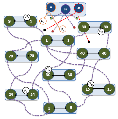
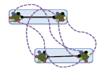
Figure 1: (a) This figure shows the distribution of the quantum signals to the different hops’nodes where the numbers on the circle represent the hops’ location. Each hop consists of entangled two nodes. The source $\mathcal{S}_{1}$, supplies the nodes randomly with different types of entangled quantum signals , Bell, $X$, pure or Werner states (dash-curves). The source $\mathcal{S}_{2}$ supplies each hop’s node with Werner state (solid curves). The source $\mathcal{S}_{3}$ supplies some nodes with unknown quantum signals $\rho_{u}$ to be teleported from one node to another using this wireless quantum network. (b) A two hops, where each hops’s node share a class of Werner state (solid-curves). Each node share a finite numbers of partial entangled quantum signals with other nodes.

2.1 Quantum Signal Distribution

As it has mentioned above, one antenna of the QMIMO sends different quantum signals to the hops’nodes. The emitted initial quantum signals to the hops’ nodes are classified as maximum entangled, partial entangled or separable states. The class of maximum entangled states (Bell states) includes $\rho_{\phi^{\pm}}=\bigl{|}\phi^{\pm}\bigr{\rangle}\bigl{\langle}\phi^{\pm}\bigr{|}$ and $\rho_{\psi^{\pm}}=\bigl{|}\psi^{\pm}\bigr{\rangle}\bigl{\langle}\psi^{\pm}\bigr{|}$, where $\bigl{|}\phi^{\pm}\bigr{\rangle}=\frac{1}{\sqrt{2}}(\bigl{|}00\bigr{\rangle}\pm\bigl{|}11\bigr{\rangle})$ and $\bigl{|}\psi^{\pm}\bigr{\rangle}=\frac{1}{\sqrt{2}}(\bigl{|}01\bigr{\rangle}\pm\bigl{|}10\bigr{\rangle})$. These entangled states can be described by using Pauli operators as [19],

$$\rho_{Bell} = \left\{\begin{array}[]{ll}\frac{1}{4}(1+\sigma_{1}^{(i)}\sigma_{1}^{(j)}+\sigma_{2}^{(i)}\sigma_{2}^{(j)}+\sigma_{3}^{(i)}\sigma_{3}^{(j)}),&\\ \frac{1}{4}(1+\sigma_{1}^{(i)}\sigma_{1}^{(j)}-\sigma_{2}^{(i)}\sigma_{2}^{(j)}+\sigma_{3}^{(i)}\sigma_{3}^{(j)}),&\\ \frac{1}{4}(1-\sigma_{1}^{(i)}\sigma_{1}^{(j)}+\sigma_{2}^{(i)}\sigma_{2}^{(j)}+\sigma_{3}^{(i)}\sigma_{3}^{(j)}),&\\ \frac{1}{4}(1-\sigma_{1}^{(i)}\sigma_{1}^{(j)}-\sigma_{2}^{(i)}\sigma_{2}^{(j)}-\sigma_{3}^{(i)}\sigma_{3}^{(j)}),&\\ \end{array}\right.$$ (5)

where $\sigma^{(i(j))}_{k},k=1,2,3$ are the Pauli operators for the qubits $"i"$ and $"j"$, respectively and $\sigma^{((i)j)}_{1}=\bigl{|}0\bigr{\rangle}\bigl{\langle}1\bigr{|}+\bigl{|}1\bigr{\rangle}\bigl{\langle}0\bigr{|}$, $\sigma^{((i)j)}_{2}=i(-\bigl{|}0\bigr{\rangle}\bigl{\langle}1\bigr{|}+\bigl{|}1\bigr{\rangle}\bigl{\langle}0\bigr{|})$ and $\sigma^{((i)j)}_{3}=\bigl{|}0\bigr{\rangle}\bigl{\langle}0\bigr{|}-\bigl{|}1\bigr{\rangle}\bigl{\langle}1\bigr{|}$. It is clear that, any one of these states can be transferred into another one by using local operations. The second types of the transmitted states from the QMIMO are partial entangled states. In this contribution, we consider two classes: $X$ and generic pure states, which can be defined as,

$$\rho_{PES} = \left\{\begin{array}[]{ll}\rho_{pure}=\frac{1}{4}\{1+p(\sigma_{1}^{(i)}-\sigma_{1}^{(j)})-\sigma_{1}^{(i)}\sigma_{1}^{(j)}-q(\sigma_{2}^{(i)}\sigma_{2}^{(j)}+\sigma_{3}^{(i)}\sigma_{3}^{(j)})\},&\\ \rho_{X}=\frac{1}{4}\{1-c^{(ij)}_{11}\sigma_{1}^{(i)}\sigma_{1}^{(j)}-c^{(ij)}_{22}\sigma_{2}^{(i)}\sigma_{2}^{(j)}-c^{(ij)}_{33}\sigma_{3}^{(i)}\sigma_{3}^{(j)}\},&\\ \end{array}\right.$$ (8)

where $p=\sqrt{1-q^{2}}$. It is clear that, if we set $p=0$ in $\rho_{pure}$, one gets a maximum entangled state (fourth state (Eq.(1)). This entangled pure state turns into a separable state if we set $p=1$. However, this type of the pure states can be transformed into four equivalent forms by local operations and consequently all the maximum entangled states can be obtained from the other forms of these pure states [20]. The degree of entanglement of this pure state is given by Wootter’s concurrence [23] as,

$$\mathcal{C}_{pure}=max\Bigl{\{}0,\frac{1}{2}(1+2q)-\frac{1}{2}\Bigr{\}}.$$ (9)

The second type of the transmitted partial entangled states is called $X-state$ [21], where one can obtain what is called Werner state [22], $\rho_{w}$ by setting $c_{11}=c_{22}=c_{33}=x$ and $\rho_{Bell}$ if we set $x=1$. The degree of entanglement of the $X-$ state is given by,

$$\mathcal{C}_{X}=max\Bigl{\{}0,\frac{3}{2}tr\{\mathord{\begin{picture}(12.0,12.0)(-1.0,0.0)\put(-1.0,9.0){\makebox(0.0,0.0)[t]{$\scriptscriptstyle\downarrow$}} \put(-1.0,9.0){\makebox(0.0,0.0)[l]{$\scriptscriptstyle\longrightarrow$}} \put(5.0,0.0){\makebox(0.0,0.0)[b]{$C$}} \end{picture}}^{\mathsf{T}}{\mathord{\begin{picture}(12.0,12.0)(-1.0,0.0)\put(-1.0,9.0){\makebox(0.0,0.0)[t]{$\scriptscriptstyle\downarrow$}} \put(-1.0,9.0){\makebox(0.0,0.0)[l]{$\scriptscriptstyle\longrightarrow$}} \put(5.0,0.0){\makebox(0.0,0.0)[b]{$C$}} \end{picture}}}\}-\frac{1}{2}\Bigr{\}},$$ (10)

where $\mathord{\begin{picture}(12.0,12.0)(-1.0,0.0)\put(-1.0,9.0){\makebox(0.0,0.0)[t]{$\scriptscriptstyle\downarrow$}} \put(-1.0,9.0){\makebox(0.0,0.0)[l]{$\scriptscriptstyle\longrightarrow$}} \put(5.0,0.0){\makebox(0.0,0.0)[b]{$C$}} \end{picture}}$ is a $3\times 3$ matrix called cross dyadic represents the correlation between the two qubits. The non-zero elements of the cross dyadic $\mathord{\begin{picture}(12.0,12.0)(-1.0,0.0)\put(-1.0,9.0){\makebox(0.0,0.0)[t]{$\scriptscriptstyle\downarrow$}} \put(-1.0,9.0){\makebox(0.0,0.0)[l]{$\scriptscriptstyle\longrightarrow$}} \put(5.0,0.0){\makebox(0.0,0.0)[b]{$C$}} \end{picture}}$ are given by $c_{11},c_{22}$ and $c_{33}$.

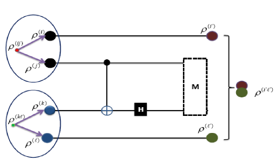
Figure 2: Circuit for generating wireless bridges between different hops.

2.2 Wireless Quantum Bridges:Entanglement Routing

Now, each node in different hops has its own qubits. The aim of this section is generating wireless quantum bridges (WQBS) between any two non-connected nodes located in different hops. This procedure can be achieved via CNOT operation and Hadamard gate followed by Bell measurements [14] as shown in Fig.(2).

Let us first consider two hops their partners share a class of $X-$ state, where the first hop’s nodes share the state $\rho^{(ij)}$ while the second hop’s nodes share the state $\rho^{(k\ell)}$. The nodes $(j)$ and $(k)$ perform CNOT operation followed by Hadamard gate on the qubit $(k)$. After performing Bell measurements on the qubits $(j\&k)$, the final state is projected into $\rho^{(i^{\prime}\ell^{\prime})}$ (see Fig.(2)). The final state $\rho^{(i^{\prime}\ell^{\prime})}$ represents the generated wireless quantum bridge between the nodes $(i\&j)$. However, if the nodes of the first and the second hops share $X-$ states, then we call the generated entangled states by $XX$ wireless bridge. In the computational basis, $00,01,10,11$, this bridge can be written as,

$$\rho_{XX}=\left(\begin{array}[]{cccc}\varrho_{11}&0&0&\varrho_{14}\\ 0&\varrho_{22}&\varrho_{23}&0\\ 0&\varrho_{32}&\varrho_{33}&0\\ \varrho_{41}&0&0&\varrho_{44}\end{array}\right),$$ (11)

where

$$\varrho_{11} = \frac{1}{2}(\mathcal{A}_{1}\mathcal{B}_{1}+\mathcal{A}_{2}\mathcal{B}_{2}),\quad\varrho_{14}=\frac{1}{2}(\mathcal{A}_{3}\mathcal{B}_{3}+\mathcal{A}_{4}\mathcal{B}_{4}),$$

$$\varrho_{22} = \frac{1}{2}(\mathcal{A}_{1}\mathcal{B}_{2}+\mathcal{A}_{2}\mathcal{B}_{1}),\quad\varrho_{23}=\frac{1}{2}(\mathcal{A}_{3}\mathcal{B}_{4}+\mathcal{A}_{4}\mathcal{B}_{3}),$$

$$\varrho_{32} = \varrho_{23},\quad\varrho_{33}=\varrho_{22},\quad\varrho_{41}=\varrho_{14},\quad\varrho_{44}=\varrho_{11},\quad\mbox{with}$$

$$\mathcal{A}_{1} = \mathcal{B}_{1}=\frac{1+c_{33}}{4},\quad\mathcal{A}_{2}=\mathcal{B}_{2}=\frac{1-c_{33}}{4},$$

$$\mathcal{A}_{3} = \mathcal{B}_{3}=\frac{c_{11}-c_{22}}{4},\quad\mathcal{A}_{4}=\mathcal{B}_{4}=\frac{c_{11}+c_{22}}{4}.$$ (12)

From this wireless quantum bridge, one can obtain the following bridges:

1. If we set $c^{(ij)}_{xx}=c^{(ij)}_{yy}=c^{(ij)}_{zz}=x$ and $c^{(k\ell)}_{11}=c^{(k\ell)}_{22}=c^{(k\ell)}_{33}=x$, one gets the wireless Werner-Werner quantum bridge ($WW$-bridge).

2. If we set $c^{(ij)}_{11}=c^{(ij)}_{22}=c^{(ij)}_{33}=x$ and $c^{(k\ell)}_{11}=c^{(k\ell)}_{22}=c^{(k\ell)}_{33}=-1$, one gets the wireless Werner-Bell quantum bridge $WB$-bridge.

3. If we set $c^{(ij)}_{11}=c^{(ij)}_{22}=c^{(ij)}_{33}=x$ and $c^{(k\ell)}_{11}\neq c^{(k\ell)}_{22}\neq c^{(k\ell)}_{33}\neq 0$ one gets the wireless Werner-$X$ quantum bridge $WX$-bridge.

However, if the node of one hop share initially $X$ state while the nodes of the another hop share a class of the generic pure state, then the generated wireless quantum bridge is called $XP$ bridge. In the computational basis, this bridge can be described by a density matrix of size $4\times 4$, its elements are given by,

$$\tilde{\varrho}_{11} = \mathcal{A}_{1}\mathcal{C}_{1}+\mathcal{A}_{2}\mathcal{C}_{2},\quad\tilde{\varrho}_{12}=-(\mathcal{A}_{1}\mathcal{C}_{3}+\mathcal{A}_{2}\mathcal{C}_{3}),\quad\tilde{\varrho}_{13}=\mathcal{C}_{3}(\mathcal{A}_{3}+\mathcal{A}_{4}),$$

$$\tilde{\varrho}_{14} = (\mathcal{A}_{3}\mathcal{C}_{1}+\mathcal{A}_{4}\mathcal{C}_{2}),\quad\tilde{\varrho}_{21}=\tilde{\varrho}_{21},\quad\tilde{\varrho}_{22}=\mathcal{A}_{1}\mathcal{C}_{2}+\mathcal{A}_{2}\mathcal{C}_{1},\quad\tilde{\varrho}_{23}=\mathcal{C}_{2}(\mathcal{A}_{3}+\mathcal{A}_{4}),\quad$$

$$\tilde{\varrho}_{24} = \tilde{\varrho}_{13}\quad\tilde{\varrho}_{23}=\tilde{\varrho}_{32},\quad\tilde{\varrho}_{33}=\tilde{\varrho}_{22},\quad\tilde{\varrho}_{34}=\tilde{\varrho}_{12},\quad\tilde{\varrho}_{41}=\tilde{\varrho}_{14},\quad\tilde{\varrho}_{42}=\tilde{\varrho}_{24}$$

$$\tilde{\varrho}_{43} = \tilde{\varrho}_{34},\quad\tilde{\varrho}_{44}=\tilde{\varrho}_{11},$$ (13)

where $\mathcal{A}_{i},i=1..4$ are given from (6) and $\mathcal{C}_{1}=\frac{1-q}{4},\quad\mathcal{C}_{2}=\frac{1+q}{4}$ and $\mathcal{C}_{3}=\frac{p}{4}$.

Fig.(3a) describes the behavior of the degree of entanglement between the terminals of the generated wireless quantum bridge (WQBS). Firstly, we assume that, the non-connected nodes share a $WW$ bridge. From this figure, we can see that the entanglement between the terminals of $WW$ bridge is generated at $x>0.578$. However, for larger values of $x$, the entanglement between the terminals of $WW$ bridge increases and reaches its maximum values, i.e., ($\mathcal{E}=1$ at $x=1$, namely, the initial states are Bell states). Secondly, the nodes of the first hop share a class of Werner type, while the second hop’s nodes share a class of $X-$ state which is defined by $c_{11}=-0.9,c_{22}=-0.8$ and $c_{33}=-0.7$. In this case, the entanglement between the terminals of the wireless quantum bridge $(WX$) is generated at $x>41$. As $x$ increases, the entanglement increases to reach its maximum value $(\mathcal{E}=0.7$ at $x=1)$. Thirdly, the nodes of one hop share a maximum entangled state (Bell types), while the second hop’s nodes share Werner state. In this case, the entanglement between the $WB$ bridge terminals is generated for smaller values of $x(=0.34)$.

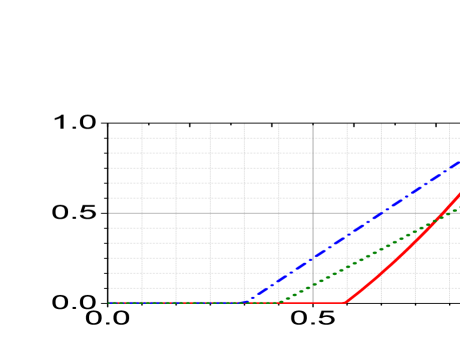
Figure 3: The entanglement $\mathcal{C}_{\mu\nu}$, of the wireless quantum bridges between the non-interacted hops. (a)The solid, dot and dash-dot curves for $WW,WX$ and $WB$, respectively. (b) The entanglement between the terminales of the wireless quantum bridge $(WP)$, where the solid, dash, dash-dot and dot curves for $p=0,0,0.9,0.7$ and $1$, respectively.

In Fig.(3b), we assume that, the hops share two different initial quantum signals. The first hop’s nodes share Werner sate, while the nodes of the second hop share a class of pure state. However, if the second hop is supplied with different initial entangled pure states, where we set $p=0,0.7,0.9,1$. It is clear that, at $p=0$, which corresponding to Bell state, the two hops entangle together at $x=0.33$. The degree of entanglement between the terminals of the wireless $WP$ bridge increases as $x$ increases to reach its maximum value ($\mathcal{E}=1$ at $x=1)$, where the initial two quantum signals are maximum entangled states. As one increases $p$, namely the second hop is supplied with less entangled pure state, the entanglement between the two hops appears suddenly for smaller values of $x$. However, the maximum values of the entanglement is reached at $x=1$, where it is smaller than ”1” for larger values of $p$. Starting from separable state, where we set $p=1$, the two hops generate a wireless quantum bridge at very small value of $x$, but the degree of entanglement between the bridge’ terminals is very small compared with those depicted for entangled pure state.

From Fig.(3), we can conclude that, it is possible to entangle different hops, their partners share arbitrary classes of initial two qubit systems. The results show that, if each hop’s nodes share a pure states even they are initially separable, one can generate entangled wireless quantum bridges between the hops’ nodes. Using Werner state with larger value of its parameter ($x>0.5$), one can generate wireless quantum bridges between the hops’ nodes with high degree of entanglement.

2.3 Bridges efficiency

In this section, we investigate the efficiency of the generated wireless quantum bridges (WQBS), where we discuss the possibility of using them as quantum channels to perform quantum teleportation. The inequality which measures the efficiency of the WQBS to perform quantum teleportation is given by [24],

$$Telp=tr\{\sqrt{\mathord{\begin{picture}(12.0,12.0)(-1.0,0.0)\put(-1.0,9.0){\makebox(0.0,0.0)[t]{$\scriptscriptstyle\downarrow$}} \put(-1.0,9.0){\makebox(0.0,0.0)[l]{$\scriptscriptstyle\longrightarrow$}} \put(5.0,0.0){\makebox(0.0,0.0)[b]{$C$}} \end{picture}}^{{}^{\mathsf{T}}}\cdot\mathord{\begin{picture}(12.0,12.0)(-1.0,0.0)\put(-1.0,9.0){\makebox(0.0,0.0)[t]{$\scriptscriptstyle\downarrow$}} \put(-1.0,9.0){\makebox(0.0,0.0)[l]{$\scriptscriptstyle\longrightarrow$}} \put(5.0,0.0){\makebox(0.0,0.0)[b]{$C$}} \end{picture}}}\}>1,$$ (14)

where the elements of the cross dyadic $\mathord{\begin{picture}(12.0,12.0)(-1.0,0.0)\put(-1.0,9.0){\makebox(0.0,0.0)[t]{$\scriptscriptstyle\downarrow$}} \put(-1.0,9.0){\makebox(0.0,0.0)[l]{$\scriptscriptstyle\longrightarrow$}} \put(5.0,0.0){\makebox(0.0,0.0)[b]{$C$}} \end{picture}}$ are given by $c_{mn}=tr\{\sigma^{(1)}_{m}\sigma^{(2)}_{n}\rho_{B}\},m,n=1,2,3$ and $\rho_{B}$ stands for the state of the wireless quantum bridge. For example, $c_{11}=tr\{\sigma_{1}^{(1)}\sigma_{1}^{(2)}\rho_{B}\}$, $c_{12}=tr\{\sigma_{1}^{(1)}\sigma_{2}^{(2)}\rho_{B}\}$ and so on,

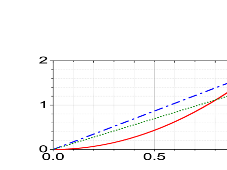
Figure 4: The efficiency of the WQBS to perform quantum teleportation.(a)The solid, dot and dash-dot for $WW,WX$ and $WB$ bridges, respectively (ba)For $WP$ bridge where, the solid, dash, dash-dot and dot curves for $p=0,0.7,0.9$,and $1$, respectively.

The behavior of teleportation inequality $(8)$, is described in Fig.(4) for different wireless quantum bridges. In Fig.(4a), the behavior of the teleportation inequality is displayed for $WW,WX$ and $WB$ bridges. It is clear that, the possibility of using the generated wireless bridges as quantum channels to perform quantum teleportation, depending on the initial degree of entanglement. However, the $WW$ bridge is useful for quantum teleportaion for $x\geq 0.8$, while $WX$ bridge for $x\geq 0.6$ and $BW$ bridge for $x\geq 0.5$. Fig.(4b) describes the behavior of the teleportation inequality (8) for $WP$ bridge. This figure shows that, the possibility of using the $WP$ bridge as quantum channel increases as $p$ decreases.

From this figure, we can find the lower values of Werner parameter $(x)$, where the generated wireless quantum bridges are useful for quantum teleportation. This means that if one can improve the efficiency of the source that sends Werner states, one can increases the efficiency of the generated wireless quantum bridges.

2.4 Teleportation

In this section, we investigate the possibility of using the more powerful wireless quantum bridges (WQBS) to teleport an unknown quantum signal given by,

$$\rho_{u}=\left(\begin{array}[]{cc}|\alpha|^{2}&\alpha\beta^{*}\\ \alpha^{*}\beta&|\beta|^{2}\end{array}\right),\quad\mbox{with}\quad|\alpha|^{2}+|\beta|^{2}=1,$$ (15)

from one hop’s partners to another. Let us first consider that, the nodes use $XX$ wireless bridge. In this case, the nodes use the state (6) as a quantum channel to perform the original protocol [25] which is based on local operations followed by Bell measurements at the sender hops’ node. These measurements are send via classical channel to the receiver’s hop, who performs some local operations depending on the received classical information. However, if the sender measures Bell state $\rho_{\phi^{+}}$, then the sent quantum signal is retrieved at receiver’s hand with a fidelity given by,

$$\mathcal{F}_{\mu\nu} = |\alpha|^{2}\Bigl{\{}(\varrho_{11}+\varrho_{22})+(\alpha\beta^{*}+\alpha^{*}\beta)(\varrho_{11}-\varrho_{22})\Bigr{\}}$$ (16)

$$+\alpha^{*}\beta\bigl{\{}(|\alpha|^{2}-|\beta|^{2})(\varrho_{14}+\varrho_{23})+(\alpha\beta^{*}-\alpha^{*}\beta)*(\varrho_{14}-\varrho_{23})\Bigr{\}}$$

$$+\alpha\beta^{*}\Bigl{\{}(|\alpha|^{2}-|\beta|^{2})(\varrho_{14}+\varrho_{23})-(\alpha\beta^{*}-\alpha^{*}\beta)*(\varrho_{14}-\varrho_{23})\Bigr{\}}$$

$$+|\beta|^{2}\Bigl{\{}(\varrho_{11}+\varrho_{22})-(\alpha\beta^{*}+\alpha^{*}\beta)(\varrho_{11}-\varrho_{22})\Bigr{\}},$$

where $\mu\nu=WW,WB$ or $WX$, if the users use Werener-Werner, Werner-Bell and X-Wernner bridges, respectively.

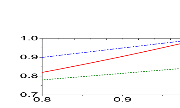
Figure 5: The fidelity of the teleported state (9) with $\alpha=\beta=\frac{1}{\sqrt{2}}$. The solid, dash and dot curves represent the fidelity, $\mathcal{F}_{\mu\nu}$ of the teleported state by using the wireless bridges $WW$, $WB$ and $WX$( $c_{xx}=-0.9,c_{yy}=-0.8,c_{zz}=-0.7$), respectively.

Fig.(5), describes the behavior of the fidelity of the teleported quantum signal via the wireless quantum bridge $WW$ (solid-curve), $WB$ bridge(dash-dot curve) and $WX$ bridge (dot curve), where we consider only the bridges which are generated at $x\geq 0.7$ (efficient bridges for teleportation). It is clear that, the initial fidelity of the teleported state depends on the initial entanglement. As an example, if the partners use the $WB$ bridge with($x\geq 0.7)$, the initial fidelity of the teleported quantum signal is large. However, as $x$ increases, the fidelity $\mathcal{F}_{\mu\nu}$ increases to reach its maximum value ($\mathcal{F}_{\mu\nu}=1$ at $x=1$). On the other hand, if the partners use the wireless $WW$ bridge, then the initial fidelity is smaller than the previous case. As the Werener’s parameter $x$ increases, the fidelity increases to become maximum at $x=1$, namely, the initially states of the two hops’ members turn into Bell states. Finally, the users use the generated $WX$ bridge then the initially fidelity depends on the degree of entanglement of $X-$ state. However, the fidelity increases as $x$ increases to reach its maximum bounds.

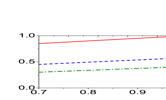
Figure 6: The same as Fig.(5), but the users use the wireless $WP$ bridge. The solid, dash and dash-dot curves for $p=0,0.7$ and $0.9$, respectively.

Finally, if the users decide to use the wireless quantum bridge $(WP)$ to teleport the unknown quantum signal (9) with a fidelity given by,

$$\mathcal{F}_{WP} = \alpha^{2}\Bigl{\{}\tilde{\varrho}_{11}+\tilde{\varrho}_{22}+2(\alpha^{2}-\beta^{2})\tilde{\varrho}_{24}+(\alpha^{*}\beta+\beta^{*}\alpha)(\tilde{\varrho}_{11}-\tilde{\varrho}_{22})\Bigr{\}}$$ (17)

$$+(\alpha^{*}\beta+\beta^{*}\alpha)\Bigl{\{}(\alpha^{2}-\beta^{2})(\tilde{\varrho}_{23}-\tilde{\varrho}_{14})-(\alpha^{*}\beta+\beta^{*}\alpha)\tilde{\varrho}_{23}-2\tilde{\varrho}_{12}\Bigr{\}}$$

$$+\beta^{2}\Bigl{\{}\tilde{\varrho}_{11}+\tilde{\varrho}_{22}+2(\alpha^{2}-\beta^{2})\tilde{\varrho}_{24}-(\alpha^{*}\beta+\beta^{*}\alpha)(\tilde{\varrho}_{11}-\tilde{\varrho}_{22})\Bigr{\}}$$

Fig.(6) shows the behavior of the fidelity $\mathcal{F}_{WP}$. The behavior shows that, the initial fidelity depends on the parameter $p$, where for $p=0$ the pure state turns into a Bell state. Therefore, the initial fidelity of the teleported state $\mathcal{F}_{WP}$ is larger. This fidelity reaches its maximum value ($\mathcal{F}_{WP}=1$ at $x=1$), which means that the two hops share a Bell state. However as $p$ increases, the initial fidelity of the teleported state decreases and the maximum bounds are reached at $x=1$. The maximum bounds decreases as $p$ increases.

3 Purification

Quantum purification has been used to distill small number of strongly entangled qubits from a large number of weakly entangled qubits, via local operations, classical communication and measurements. The first purification protocol (IBM) has proposed by Bennett et al.[26], where they obtain the singled states from Werner classes. Deutsch et al. [27] have suggested the Oxford protocol which is more efficient than IBM protocol. Since then there are several protocols have been suggested. For example, a more efficient entanglement purification protocol is suggested by Metwally[28], which is more efficient than the IBM and Oxford protocols. Another improvement has been done on the IBM protocol by Feng et al.[29]. All the previous protocol have been improved by several versions. Among of these improvements the protocol which is introduced by Metwally and Obada [30], where this improved version based on using the controlled-controlled NOT gate (CCNOT) instead of CNOT.

In this context, we can use one of the previous protocols to distill a wireless quantum bridges with high degree of entanglement from weakly entangled bridges. In this wireless quantum network, we suggested two strategies: The first is the initial partial entangled state can be purified before sending them to the hops’nodes. In this case, all the users will be supplied by MES, and the protocol turns into Wang et al. protocol [17]. The second possibility is performing a quantum purification protocol on the less entangled bridges (useless bridges for teleportation) to increase their efficiency. However this will be our next contribution to find which strategy is better.

4 Conclusion

The possibility of generating wireless quantum networks (WQNS) between different hops’nodes, where it is assumed that these nodes share together arbitrary two qubit systems randomly, is discussed. To achieve quantum communication between the non-connected hops’nodes, the users have to generated wireless quantum bridges. The type of these Wireless bridges depends on the states which are shared between the terminals of each hop, where we have generated Werner-Werner, Werner-Bell,Werner- $X$ and Werner-Pure bridges. The entanglement of each WQB is quantified by the means of concurrence. It is shown that, for less entangled state the non-connected hops’ nodes turn into wireless quantum bridges for larger values of Werener’s parameter, $x$. However, the partial entangled wireless quantum bridges turn into a maximum entangled wireless bridges when the Werner’s parameter namely ($x=1$). The entanglement of the Werner-Pure (WP) bridges, depends on pure and Werner states’s parameters, where it increases for larger values of Werner parameter and smaller values of the pure state parameter.

The efficiency of the generated wireless quantum bridges to perform quantum teleportation is discussed for different types of bridges. It is shown that, the teleportation inequality is violated for small values of the Werner’s parameter and consequently the efficiency of the WQBS to perform quantum teleportation decreases. However, this efficiency of the generated wireless quantum bridges increase for larger values of Werner’s parameter and smaller values of the pure state’s parameter.

The more powerful wireless quantum bridges are used to teleport unknown quantum signals from one node to another, where we consider only the bridges which obey the teleportation inequality. The fidelity of the teleported quantum signal increases by increasing Werner’s parameter or decreasing the pure state parameter for $WP$ bridge. The maximum value of the fidelity depends on the entanglement of the used wireless quantum bridge.

In conclusion: a wireless quantum networks (WQNS) can be generated between different hops’ nodes sharing arbitrary different two qubit states. The efficiency of the WQN and hence its ability to perform wireless quantum communication can be enhanced by controlling the devices which generate these signals.

References

- [1] H. Yang, F. Ricciato, S. Lu, and L. Zhang, ” Securing wireless world”, Proceeding IEEE 94 442-454 (2006).
- [2] P. Hemmer, ” Closer to Quantum Internet”, Physics, 6 62-64 (2013).
- [3] O. Giraud, B. Georgeot and D. L. Shepelynasky, ” Quantum computing of delocalization in small-world networks”, Phys. Rev. E. 036303 (2005).
- [4] O. Mülken, V. Pernic and A. Blumen, ” Quantum transport on small-word networks:A continuous-time quantum walk approch”, Phys. Rev. E 76 51125 (2007).
- [5] S. M. Platten, M,. A. Lohe and P. J. Moran,” Multiple frequencies of synchronization in classical and quantum network”, Phys. Rev. E 85 026207 (2011).
- [6] A. Halu, S. Garnerone, A. Vezzani and G. Bianconi,” Phase transition of light on complex quantum network”, Phys. Rev. E 87 022104 (2013).
- [7] D. Zueco, F. Galve, S. Kohler and P. Häggi,” Quantum router on ac control of qubit chain”, Phys. Rev. A80 042303-042313 (2009).
- [8] L.-M. Duan and Monroe,” Colloquium: Quantum networks with trapped ions”, Rev. Mod. Phys. 82 1209-1224 (2010).
- [9] S. Sergeenkov and G. Rotoli, ” Wireless connection between Josephson qubits”, Phys. Rev. A 79 044301- 044304 (2009).
- [10] C. Chudzicki and F. W. Strauch” Parallel State transfere and Efficient of Quantum Routing on Quantum Networks”, Phys. Rev. Lett. 105 260501-260504 (2010).
- [11] P. P.-Ross, A. Kay,” Perfect Quantum Routing in Regaular Spin Network”, Phys. Rev. Lett. 106 020503-020506 (2011).
- [12] N. Metwally, ”Entangled Network and Quantum Communication”, Phys. Lett. A 375 4268-4273 (2011).
- [13] A. Abdel-Aty, N. Zakaria, L. Cheong and N. Metwally,” Effect of Spin-Orbit Interaction (Heisenberg XYZ Model) On partial entangled Quantum Network”, Quant. Inf. Sci. 4 1-17 (2014).
- [14] S.-T. Cheng, C. Yen Wang and M,-Hon Tao” Quantum Communication for wireless Wide-Area Network”, IEEE Journal, 3 1424-1432 (2005).
- [15] S. Paganelli, S. Lorenzo, T. Appollaro, F. Plastina and G. Giorgi,”Routing quantum Information in Spin chains”, Phys. Rev. A 87 062309-062316 (2013).
- [16] Yu-Xu-Tao, Xu Jin and Zhang Zai-Chen, ” Distribited wireless quantum communication network”, Cin. Phys. B 22 090311-090317 (2013).
- [17] K. Wang, Xu-Tao-Yu, Sheng-Li-Lu, and Yan-Xiao Gong,” Quantum wireless multi Hop communicatioon based on arbitrary Bell pairs and teleportation”, Phys. Rev. A 89 022329-022339 (2014).
- [18] Liang Wu and Shigun Zhu, ” Entanglement percolation on a quantum internet with scale-free and clustreing characters”, Phys. Rev. A. 84 052304- 052309 (2011).
- [19] M. A. Nielsen and I. L. Chuang ”,Quantum Computation and Quantum Information” (Cambridge University Press, Cambridge UK (2010).
- [20] B. -G. Englert and N. Metwally,”Seperability of entangled q-bit pairs” J. Mod. Opt. 47 2221- (2000); B. -G. Englert and N. Metwally,” Remarks on 2-qubit states”, Appl. Phys.B 72 35- (2001).
- [21] T. Yu and J. H. Eberly ” Evolution from entanglement to decohetrenceof bipartite mixed ”” states”, Quantum Inform. Comput 7, 459 (2007).
- [22] R. F. Werner,” Quantum states with Einstein-Podolsky-Rosen correlations admitting a hidden-variable model”, Phys. Rev. A 40 4277-4281 (1989).
- [23] W. K. Woottors,” Entanglement of formation of an arbitrary state of two qubit”, Phys. Rev. Lett. 80 2245 (1998).
- [24] R. Horodeckia, P. Horodeckib, M. Horodecki, ”Violating Bell inequality by mixed View the MathML source states: necessary and sufficient condition”, Phys. Lett. A 200 340 344 (1995).
- [25] C. Bennett, C. Brassard, C. Crpeau, R. josa, A. Peres and W. K. Woottors” Teleporting an unknown quantum state via dual classical and Einstein- Podolosky- Rosen channel”, Phys. Rev. Lett. 70 1895-1899 (1993 ).
- [26] C. H. Bennett, G, Brassard, S. Popescu, B. Schoumacher, J. I. Somlin and W. K. Woottors, ”Mixed-state entanglement and quantum error correction ”, Phys. Rev. A 54 3284-3851 (1996).
- [27] D. Deutch, A. Ekert, R. Jozsa, C. Macchiavello, S. Popescu and A. Sanpera,” Quantum Privacy Ampli?cation and the Security of Quantum Cryptography over Noisy Channels”, Phys. Rev. Lett. 77 2818-2821 (1996).
- [28] N. Metwally,” More efficient entanglement purification”, Phys. Rev. A 66 054302-054305 (2002).
- [29] Xun-Li Feng, Shang-Qing Gong, Zhi-Zhan Xu,”Quantum Privacy Ampli?cation and the Security of Quantum Cryptography over Noisy Channels”, Phys. Lett. A 271 44 (2000).
- [30] N. Metwally and A. -S. Obada, ” More efficient purifying scheme via controlled-controlled NOT gate”, Phys. Lett. A 352 45-48 (2006).