Fatal Attractors in Parity Games:

Building Blocks for Partial Solvers

Michael Huth, Jim Huan-Pu Kuo, and Nir Piterman 

18 May 2014

Abstract: Formal methods and verification rely heavily on algorithms that compute which states of a model satisfy a specified property. The underlying decision problems are often undecidable or have prohibitive complexity. Consequently, many algorithms represent partial solvers that may not terminate or report inconclusive results on some inputs but whose terminating, conclusive outputs are correct. It is therefore surprising that partial solvers have not yet been studied in verification based on parity games, a problem that is known to be polynomial-time equivalent to the model checking for modal mu-calculus. We here provide what appears to be the first such in-depth technical study by developing the required foundations for such an approach to solving parity games and by experimentally validating the utility of these foundations.

Attractors in parity games are a technical device for solving “alternating” reachability of given node sets. A well known solver of parity games – Zielonka’s algorithm – uses such attractor computations recursively. We here propose new forms of attractors that are monotone in that they are aware of specific static patterns of colors encountered in reaching a given node set in alternating fashion. Then we demonstrate how these new forms of attractors can be embedded within greatest fixed-point computations to design solvers of parity games that run in polynomial time but are partial in that they may not decide the winning status of all nodes in the input game.

Experimental results show that our partial solvers completely solve benchmarks that were constructed to challenge existing full solvers. Our partial solvers also have encouraging run times in practice. For one partial solver we prove that its runtime is at most cubic in the number of nodes in the parity game, that its output game is independent of the order in which monotone attractors are computed, and that it solves all Büchi games and weak games.

We then define and study a transformation that converts partial solvers into more precise partial solvers, and we prove that this transformation is sound under very reasonable conditions on the input partial solvers. Noting that one of our partial solvers meets these conditions, we apply its transformation on $1.6$ million randomly generated games and so experimentally validate that the transformation can be very effective in increasing the precision of partial solvers.

1 Introduction

Formal methods are by now an accepted means of verifying the correctness of computing artifacts such as software (e.g. [BLR11]), protocol specifications (e.g. [Bla09], system architectures (e.g. [BG08]), behavioral specifications (e.g. [UABD⁺13]), etc.. Model checking [CE81, QS82] is arguably one of the success stories of formal methods in this context. In that approach, one expresses the artifact as a model $M$, the property to be analyzed as a formula $\phi$, and then can check whether $M$ satisfies $\phi$ through an automated analysis. It is well understood [EJS93, Sti95] that model checking of an expressive fixed-point logic, the modal mu-calculus [Koz83], is equivalent (within polynomial time) to the solving of parity games.

A key obstacle to the effectiveness of model checking and game-based verification is that the underlying decision problems are typically undecidable (e.g. for many types of infinite-state systems [BE01]) or have prohibitive complexity (e.g. subexponential algorithms for solving parity games [JPZ08]). Abstraction is seen as an important technique for addressing these challenges. Program analyses are a good example of this: a live variable analysis (see e.g. [NNH99]) has as output statements about the liveness of program variables at program points. These statements are of form “variable $x$ may be live at program point $p$” and “$x$ is not live at $p$”, but that particular live-variable analysis can then not produce statements of form “$x$ is definitely live at $p$”. This limitation trades off undecidability of the underlying decision problem “is $x$ live at $p$?” with the precision of the answer.

Abstraction of models is another prominent technique for making such trade-offs [CGL94, CGJ⁺03]: instead of verifying that model $M$ satisfies $\phi$, we may abstract $M$ to some model $A$ and verify $\phi$ on $A$ instead of on $M$. A successful verification on $A$ will then mean that $\phi$ is also verified for $M$. Failure to verify $\phi$ on $A$ may provide diagnostic evidence for failure of $\phi$ on $M$, but it may alternatively mean that we don’t know whether $M$ satisfies $\phi$ or not. So this is again trading off the precision of the analysis with its complexity: even a verification algorithm that is linear in the size of $M$ cannot be run on $M$ if the latter is prohibitively large; but we have to accept that verification on a much smaller abstraction may be inconclusive for the $M$ in question.

In light of this state of the art in formal verification, we think it is really surprising that no prior research appears to exist on algorithms that solve parity games by trading off the precision of the solution with its complexity. Let us first discuss parity games at an abstract level before we detail how such a trade off may work in this setting. Mathematically, parity games (see e.g. [Zie98]) can be seen as a representation of the model checking problem for the modal mu-calculus [EJS93, Sti95], and its exact computational complexity has been an open problem for over twenty years now. The decision problem of which player wins a given node in a given parity game is known to be in UP$\cap$coUP [Jur98].

Parity games are infinite, $2$-person, $0$-sum, graph-based games. Nodes are controlled by different players (player $0$ and player $1$), are colored with natural numbers, and the winning condition of plays in the game graph depends on the minimal color occurring in cycles. A fundamental result about parity games states that these games are determined [Mos91, EJ91, Zie98]: each node in a parity game is won by exactly one of the players $0$ or $1$. Moreover, each player has a non-randomized, memoryless strategy that guarantees her to win from every node that she can indeed win in that game [Mos91, EJ91, Zie98]. The condition for winning a node, however, is an alternation of existential and universal quantification. In practice, this means that the maximal color of its coloring function is the only exponential source for the worst-case complexity of most parity game solvers, e.g. for those in [Zie98, Jur00, VJ00].

We suggest that research on solving parity games may be loosely grouped into the following different methodological approaches:

• design of algorithms that solve all parity games by construction and that so far all have exponential or sub-exponential worst-case complexity (e.g. [Zie98, Jur00, VJ00, JPZ08]),

• restriction of parity games to classes for which polynomial-time algorithms can be devised as complete solvers (e.g. [BDHK06, DKT12]), and

• practical improvements to solvers so that they perform well across benchmarks (e.g. [FL09]).

We here propose a new methodology for researching solutions to parity games. We want to design and evaluate a new form of “partial” parity game solver. These are solvers that are well defined for all parity games, are guaranteed to run in time polynomial in the size of the input game, but that may not solve all games completely – i.e. for some parity games they may not decide the winning status of some nodes. In this approach, a partial solver has an arbitrary parity game as input and returns two things:

1. a sub-game of the input game, and

2. a decision on the winner of nodes from the input game that are not in that sub-game.

In particular, the returned sub-game is empty if, and only if, the partial solver classified the winners for all input nodes. The input/output type of our partial solvers clearly relates them to so called preprocessors that may decide the winner of nodes whose structure makes such a decision an easy static criterion (e.g. in the elimination of self-loops or dead ends [FL09]). But we here search for algorithmic building blocks from which we can construct efficient partial solvers that completely solve a range of benchmarks of parity games. This ambition sets our work apart from research on preprocessors but is consistent with it as one can, in principle, run a partial solver as preprocessor.

The motivation for the study reported in this paper is therefore that we want to investigate what algorithmic building blocks one may create and use for designing partial solvers that run in polynomial time and work well on many games, whether there are interesting subclasses of parity games for which partial solvers completely solve all game, and whether the insights gained in this study may lead to an understanding of whether partial solvers can be components of more efficient complete solvers.

We now summarize the main contributions made in this paper. We present a new form of attractor that can be used in fixed-point computations to detect winning nodes for a given player in parity games. Then we propose several designs of partial solvers for parity games by using this new attractor within greatest fixed-point computations. Next, we analyze these partial solvers and show, amongst other things, that they work in PTIME and that one of them is independent of the order of attractor computation. We then evaluate these partial solvers against known benchmarks and report that these experiments have very encouraging results. Next, we define a function that transforms partial solvers on that class of games to more precise partial solvers. Finally, we experimentally evaluate this transformation for the most efficient partial solver we proposed in this study and report that these experiments are very encouraging.

Outline of paper. Section 2 contains needed formal background and fixes notation. Section 3 introduces the building block of our partial solvers, a new form of attractor. Some partial solvers based on this attractor are presented in Section 4, theoretical results about these partial solvers are proved in Section 5, and experimental results for these partial solvers run on benchmarks are reported and discussed in Section 6. The transformation of partial solvers is presented in Section 7, where we also analyze and experimentally evaluate this transformation. We summarize and conclude the paper in Section 8.

2 Preliminaries

We write $\mathbb{N}$ for the set $\{0,1,\dots\}$ of natural numbers. A parity game $G$ is a tuple $(V,V_{0},V_{1},E,c)$, where $V$ is a set of nodes partitioned into possibly empty node sets $V_{0}$ and $V_{1}$, with an edge relation $E\subseteq V\times V$ (where for all $v$ in $V$ there is a $w$ in $V$ with $(v,w)$ in $E$), and a coloring function $c\colon V\to\mathbb{N}$. In figures, $c(v)$ is written within nodes $v$, nodes in $V_{0}$ are depicted as circles and nodes in $V_{1}$ as squares. For $v$ in $V$, we write $v.E$ for node set $\{w\in V\mid(v,w)\in E\}$ of successors of $v$. By abuse of language, we call a subset $U$ of $V$ a sub-game of $G$ if the game graph $(U,E\cap(U\times U))$ is such that all nodes in $U$ have some successor. We write ${\mathcal{P}G}$ for the class of all finite parity games $G$, which includes the parity game with empty node set for our convenience. We only consider games in ${\mathcal{P}G}$.

Throughout, we write $p$ for one of $0$ or $1$ and $1-p$ for the other player. In a parity game, player $p$ owns the nodes in $V_{p}$. A play from some node $v_{0}$ results in an infinite play $r=v_{0}v_{1}\dots$ in $(V,E)$ where the player who owns $v_{i}$ chooses the successor $v_{i+1}$ such that $(v_{i},v_{i+1})$ is in $E$. Let $\mathsf{Inf}({r})$ be the set of colors that occur in $r$ infinitely often:

$$\mathsf{Inf}({r})=\{k\in\mathbb{N}\mid\forall j\in\mathbb{N}\colon\exists i\in\mathbb{N}\colon i>j\mbox{ and }k=c(v_{i})\}$$

Player $0$ wins play $r$ iff $\min\mathsf{Inf}({P})$ is even; otherwise player $1$ wins play $r$.

A strategy for player $p$ is a total function $\tau\colon V_{p}\to V$ such that $(v,\tau(v))$ is in $E$ for all $v\in V_{p}$. A play $r$ is consistent with $\tau$ if each node $v_{i}$ in $r$ owned by player $p$ satisfies $v_{i+1}=\tau(v_{i})$. It is well known that each parity game is determined: node set $V$ is the disjoint union of two, possibly empty, sets $W_{0}$ and $W_{1}$, the winning regions of players $0$ and $1$ (respectively). Moreover, strategies $\sigma\colon V_{0}\to V$ and $\pi\colon V_{1}\to V$ can be computed such that

• all plays beginning in $W_{0}$ and consistent with $\sigma$ are won by player $0$; and

• all plays beginning in $W_{1}$ and consistent with $\pi$ are won by player $1$.

Solving a parity game means computing such data $(W_{0},W_{1},\sigma,\pi)$.

Example 1

In the parity game $G$ depicted in Figure 1, the winning regions are $W_{1}=\{v_{3},v_{5},v_{7}\}$ and $W_{0}=\{v_{0},v_{1},v_{2},v_{4},v_{6},v_{8},v_{9},v_{10},v_{11}\}$. Let $\sigma$ move from $v_{2}$ to $v_{4}$, from $v_{6}$ to $v_{8}$, from $v_{9}$ to $v_{8}$, and from $v_{10}$ to $v_{9}$. Then $\sigma$ is a winning strategy for player $0$ on $W_{0}$. And every strategy $\pi$ is winning for player $1$ on $W_{1}$.

3 Fatal attractors

In this section we define a special type of attractor that is used for our partial solvers in the next section. We start by recalling the normal definition of attractor, and that of a trap, and then generalize the former to our purposes.

Definition 1

Let $X$ be a node set in parity game $G$. For player $p$ in $\{0,1\}$, set

$${\mathsf{cpre}_{p}({X})} = \{v\in V_{p}\mid v.E\cap X\neq\emptyset\}\cup\{v\in V_{1-p}\mid v.E\subseteq X\}$$ (1)

$${{\mathsf{Attr}}_{{p}}[{G},{X}]} = \mu Z.(X\cup{\mathsf{cpre}_{p}({Z})})$$ (2)

where $\mu Z.F(Z)$ denotes the least fixed point of a monotone function $F\colon(2^{V},\subseteq)\to(2^{V},\subseteq)$.

The control predecessor of a node set $X$ for $p$ in (1) is the set of nodes from which player $p$ can force to get to $X$ in exactly one move. The attractor for player $p$ to a set $X$ in (2) is computed via a least fixed-point as the set of nodes from which player $p$ can force the game in zero or more moves to get to the set $X$. Dually, a trap for player $p$ is a region from which player $p$ cannot escape.

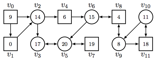
Figure 1: A parity game: circles denote nodes in $V_{0}$, squares denote nodes in $V_{1}$.

Definition 2

Node set $X$ in parity game $G$ is a trap for player $p$ ($p$-trap) if for all $v\in V_{p}\cap X$ we have $v.E\subseteq X$ and for all $v\in V_{1-p}\cap X$ we have $v.E\cap X\neq\emptyset$.

It is well known that the complement of an attractor for player $p$ is a $p$-trap and that it is a sub-game. We state this here formally as a reference:

Theorem 1

Given a node set $X$ in a parity game $G$, the set $V\setminus{{\mathsf{Attr}}_{{p}}[{G},{X}]}$ is a $p$-trap and a sub-game of $G$.

We now define a new type of attractor, which will be a crucial ingredient in the definition of all our partial solvers developed in this paper.

Definition 3

Let $A$ and $X$ be node sets in parity game $G$, let $p$ in $\{0,1\}$ be a player, and $c$ a color in $G$. We set

$${{{\mathsf{mpre}}}_{p}({A},{X},{c})} = \{v\in V_{p}\mid c(v)\geq c\land v.E\cap(A\cup X)\neq\emptyset\}\cup$$

$$\{v\in V_{1-p}\mid c(v)\geq c\land v.E\subseteq A\cup X\}$$

$${{{{\mathsf{MAttr}}}}_{p}({X},{c})} = \mu Z.{{{\mathsf{mpre}}}_{p}({Z},{X},{c})}$$ (3)

The monotone control predecessor ${{{\mathsf{mpre}}}_{p}({A},{X},{c})}$ of node set $A$ for $p$ with target $X$ is the set of nodes of color at least $c$ from which player $p$ can force to get to either $A$ or $X$ in one move. The monotone attractor ${{{{\mathsf{MAttr}}}}_{p}({X},{c})}$ for $p$ with target $X$ is the set of nodes from which player $p$ can force the game in one or more moves to $X$ by only meeting nodes whose color is at least $c$. Notice that the target set $X$ is kept external to the attractor. Thus, if some node $x$ in $X$ is included in ${{{{\mathsf{MAttr}}}}_{p}({X},{c})}$ it is so as it is attracted to $X$ in at least one step.

Our control predecessor and attractor are different from the “normal” ones in a few ways. First, ours take into account the color $c$ as a formal parameter. They add only nodes that have color at least $c$. Second, as discussed above, the target set $X$ itself is not included in the computation by default. For example, ${{{{\mathsf{MAttr}}}}_{p}({X},{c})}$ includes states from $X$ only if they can be attracted to $X$.

We now show the main usage of this new operator by studying how specific instantiations thereof can compute so called fatal attractors.

Definition 4

Let $X$ be a set of nodes of color $c$, where $p=c\%2$.

1. For such an $X$ we denote $p$ by $p(X)$ and $c$ by $c(X)$. We denote ${{{{\mathsf{MAttr}}}}_{p}({X},{c})}$ by ${\mathsf{MA}({X})}$. If $X=\{x\}$ is a singleton, we denote ${\mathsf{MA}({X})}$ by ${\mathsf{MA}({x})}$.

2. We say that ${\mathsf{MA}({X})}$ is a fatal attractor if $X\subseteq{\mathsf{MA}({X})}$.

We record and prove that fatal attractors ${\mathsf{MA}({X})}$ are node sets that are won by player $p(X)$ in $G$:

Theorem 2

Let ${\mathsf{MA}({X})}$ be fatal in parity game $G$. Then the attractor strategy for player $p(X)$ on ${\mathsf{MA}({X})}$ is winning for $p(X)$ on ${\mathsf{MA}({X})}$ in $G$.

Proof: The winning strategy is the attractor strategy corresponding to the least fixed-point computation in ${{{{\mathsf{MAttr}}}}_{p}({X},{c})}$. First of all, player $p(X)$ can force, from all nodes in ${\mathsf{MA}({X})}$, to reach some node in $X$ in at least one move. Then, player $p(X)$ can do this again from this node in $X$ as $X$ is a subset of ${\mathsf{MA}({X})}$. At the same time, by definition of ${{{{\mathsf{MAttr}}}}_{p}({X},{c})}$ and ${{{\mathsf{mpre}}}_{p}({A},{X},{c})}$, the attraction ensures that only colors of value at least $c$ are encountered. So in plays starting in ${\mathsf{MA}({X})}$ and consistent with that strategy, every visit to a node of parity $1-p(X)$ is followed later by a visit to a node of color $c(X)$. It follows that in an infinite play consistent with this strategy and starting in ${\mathsf{MA}({X})}$, the minimal color to be visited infinitely often is $c$ – which is of $p$’s parity. $\blacksquare$

Let us consider the case when $X$ is a singleton $\{k\}$ and ${\mathsf{MA}({k})}$ is not fatal. We show that, under a certain condition, we can remove an edge from $G$ without changing the set of winning strategies or winning regions of either player:

Lemma 1

Let ${\mathsf{MA}({k})}$ be not fatal for node $k$. Then we may remove edge $(k,w)$ in $E$ if $w$ is in ${\mathsf{MA}({k})}$, without changing winning regions of parity game $G$.

Proof: Suppose that there is an edge $(k,w)$ in $E$ with $w$ in ${\mathsf{MA}({k})}$. We show that this edge cannot be part of a winning strategy (of either player) in $G$. Since ${\mathsf{MA}({k})}$ is not fatal, $k$ must be in $V_{1-p(k)}$ and so is controlled by player $1-p(k)$. But if that player were to move from $k$ to $w$ in a memoryless strategy, player $p(k)$ could then attract the play from $w$ back to $k$ without visiting colors of parity $1-p(k)$ and smaller than $c(k)$, since $w$ is in ${\mathsf{MA}({k})}$. And, by the existence of memoryless winning strategies [EJ91], this would ensure that the play is won by player $p(k)$ as the minimal infinitely occurring color would have parity $p(k)$. $\blacksquare$

Example 2

For $G$ in Figure 1, the only colors $k$ for which ${\mathsf{MA}({k})}$ is fatal are $4$ and $8$: monotone attractor ${\mathsf{MA}({4})}$ equals $\{v_{2},v_{4},v_{6},v_{8},v_{9},v_{10},v_{11}\}$ and monotone attractor ${\mathsf{MA}({8})}$ equals $\{v_{9},v_{10},v_{11}\}$. In particular, ${\mathsf{MA}({8})}$ is contained in ${\mathsf{MA}({4})}$ and nodes $v_{1}$ and $v_{0}$ are attracted to ${\mathsf{MA}({4})}$ in $G$ by player $0$. And $v_{11}$ is in ${\mathsf{MA}({11})}$ (but the node of color 11, $v_{10}$, is not), so edge $(v_{10},v_{11})$ may be removed.

4 Partial solvers

We can use the above definitions and results to define partial solvers next. In doing so, we will also prove their soundness. Throughout this paper, pseudo-code of partial solvers will not show the routine code for accumulating detected winning regions and their corresponding winning strategies – their nature will be clear from our discussions and soundness proofs.

4.1 Partial solver psol

Figure 2 shows the pseudocode of a partial solver, named psol, based on ${\mathsf{MA}({X})}$ for singleton sets $X$. Solver psol explores the parity game $G$ in descending color ordering. For each node $k$, it constructs ${\mathsf{MA}({k})}$, and aims to do one of two things:

• If node $k$ is in ${\mathsf{MA}({k})}$, then ${\mathsf{MA}({k})}$ is fatal for player $1-p(k)$, thus node set ${{\mathsf{Attr}}_{{p(k)}}[{G},{{\mathsf{MA}({k})}}]}$ is a winning region of player $p(k)$, and removed from $G$.

• If node $k$ is not in ${\mathsf{MA}({k})}$, and there is a $(k,w)$ in $E$ where $w$ is in ${\mathsf{MA}({k})}$, all such edges $(k,w)$ are removed from $E$ and the iteration continues.

psol($G=(V,V_{0},V_{1},\!E,c)$) {
  for ($k\in\!\!V$ in descending color ordering $c(k)$) {
    if ($k\in{{\mathsf{MA}({k})}}$) { return psol($G\!\!\setminus\!\!{{{\mathsf{Attr}}_{{p(k)}}[{G},{{\mathsf{MA}({k})}}]}}$) }
    if ($\exists\!\!(k,w)\in\!\!E\colon\!\!w\in\!{\mathsf{MA}({k})}$)
    $\{G=G\setminus\!\!\!\!\!\!\{(k,w)\in\!\!E\mid w\in\!\!{\mathsf{MA}({k})}\}\}$
  }
  return $G$
}

Figure 2: Partial solver psol based on detection of fatal attractors ${\mathsf{MA}({k})}$ and fatal moves.

If for no $k$ in $V$ attractor ${\mathsf{MA}({k})}$ is fatal, game $G$ is returned as is – empty if ${\tt psol}$ solves $G$ completely.

Example 3

In a run of psol on $G$ from Figure 1, there is no effect for colors larger than $11$. For $c=11$, psol removes edge $(v_{10},v_{11})$ as $v_{11}$ is in the monotone attractor ${\mathsf{MA}({11})}$. The next effect is for $c=8$, when the fatal attractor ${\mathsf{MA}({8})}=\{v_{9},v_{10},v_{11}\}$ is detected and removed from $G$ (the previous edge removal did not cause the attractor to be fatal). On the remaining game, the next effect occurs when $c=4$, and when the fatal attractor ${\mathsf{MA}({4})}$ is $\{v_{2},v_{4},v_{6},v_{8}\}$ in that remaining game. As player $0$ can attract $v_{0}$ and $v_{1}$ to this as well, all these nodes are removed and the remaining game has node set $\{v_{3},v_{5},v_{7}\}$. As there is no more effect of psol on that remaining game, it is returned as the output of psol’s run.

4.2 Partial solver psolB

Figure 3 shows the pseudocode of another partial solver, named psolB – the “B” suggesting a relationship to “Büchi”. This partial solver is based on ${\mathsf{MA}({X})}$, where $X$ is a set of nodes of the same color. This time, the operator ${\mathsf{MA}({X})}$ is used within a greatest fixed-point in order to discover the largest set of nodes of a certain color that can be (fatally) attracted to itself. Accordingly, the greatest fixed-point starts from all the nodes of a certain color and gradually removes those that cannot be attracted to the same color. When the fixed-point stabilizes, it includes the set of nodes of the given color that can be (fatally) attracted to itself. This node set can be removed (as a winning region for player $d\%2$) and the residual game analyzed recursively. As before, the colors are explored in descending order.

psolB($G=(V,V_{0},V_{1},\!E,c)$) {
  for (colors $d$ in descending ordering) {
    $X=\{v\ inV\mid c(v)=d\,\}$;
    cache = $\{\}$;
    while ($X\neq\{\}$ && $X\neq$ cache) {
      cache = $X$;
      if ($X\subseteq{{\mathsf{MA}({X})}}$) { return psolB($G\setminus{{{\mathsf{Attr}}_{{d\%2}}[{G},{{\mathsf{MA}({X})}}]}}$)
      } else { $X$ = $X\cap\!{{\mathsf{MA}({X})}}$; }
    }
  }
  return $G$
}

Figure 3: Partial solver psolB.

We make two observations. First, if we were to replace the recursive calls in psolB with the removal of the winning region from $G$ and a continuation of the iteration, we would get an implementation that discovers less fatal attractors – we confirmed this experimentally. Second, edge removal in psol relies on the set $X$ being a singleton. A similar removal could be achieved in psolB when the size of $X$ is reduced by one (in the operation $X=X\cap{\mathsf{MA}({X})}$). Indeed, in such a case the removed node would not be removed and the current value of $X$ be realized as fatal. We have not tested this edge removal approach experimentally for this variant of psolB.

Example 4

A run of psolB on $G$ from Figure 1 has the same effect as the one for psol, except that psolB does not remove edge $(v_{10},v_{11})$ when $c=11$.

A way of comparing partial solvers $P_{1}$ and $P_{2}$ is to say that $P_{1}\leq P_{2}$ if, and only if, for all parity games $G$ the set of nodes in the output sub-game $P_{1}(G)$ is a subset of the set of nodes of the output sub-game $P_{2}(G)$. The next example shows that psol and psolB are incomparable for this intentional pre-order over partial solvers:

Example 5

Consider the game $G$ in Figure 4(a). Partial solver psolB decides no nodes in this game since the monotone attractors it computes are empty for all colors of $G_{1}$. But psol detects for $k=v_{1}$ that $v_{0}$ is in the monotone attractor of $k$ and that $v_{1}$ is not. Therefore, it removes edge $(v_{1},v_{0})$ from $G_{1}$. When it comes to evaluating $k=v_{2}$, it now detects that $v_{2}$ is in its monotone attractor and so this fatal attractor decides $\{v_{0},v_{1},v_{3}\}$. The same process repeats for $v_{3}$. We note that when psolB computes the monotone attractor of $\{v_{1},v_{3}\}$ both nodes are removed from the attractor simultaneously. Thus, our optimization of psolB that tries to remove edges when the size of the set decreases by $1$ does not apply here.

Now consider game $G^{\prime}$ in Figure 4(b). Then all monotone attractors that psol computes are empty and so it solves no nodes. But running psolB on $G^{\prime}$ now decides all nodes since it detects for $d=0$ and $X=\{v_{0},v_{2}\}$ a fatal attractor for all nodes.

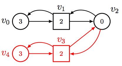
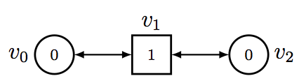
Figure 4: Subfigure (a): a game that psolB cannot solve at all and that psol solves completely. Subfigure (b): a game that psol cannot solve at all but that psolB solves completely.

Let us introduce some notation for the regions of nodes that are decided by partial solves.

Definition 5

Let $G$ be a parity game, ${\mathsf{\rho}}$ a partial solver, and $p$ in $\{0,1\}$ a player in $G$. Then ${{\mathsf{Win}}_{{{\mathsf{\rho}}}}[{G},{s}]}$ denotes the set of nodes in $G$ that ${\mathsf{\rho}}$ classifies as being won by player $p$ in $G$.

Next, we state that both psolB and psol are sound partial solver.

Theorem 3

The partial solvers psolB and psol are sound: let $G$ be a parity game. Then ${{\mathsf{Win}}_{{{\tt psol}}}[{G},{0}]}$ and ${{\mathsf{Win}}_{{{\tt psol}}}[{G},{0}]}$ are contained in the winning region of player $0$ in $G$, and ${{\mathsf{Win}}_{{{\tt psolB}}}[{G},{1}]}$ and ${{\mathsf{Win}}_{{{\tt psolB}}}[{G},{1}]}$ are contained in the winning region of player $1$ in $G$.

Proof:

1. We prove the claim for psolB first. Let $G$ be a parity game. In Theorem 2, we have proved that ${\mathsf{MA}({X})}$ is winning for player $p(X)$ if $X$ is a subset of ${\mathsf{MA}({X})}$. For every color $d$ in $G$, the for-loop in psolB constructs ${\mathsf{MA}({X})}$ where all nodes in $X$ have color $d$. If $X$ is a subset of ${\mathsf{MA}({X})}$, then ${\mathsf{MA}({X})}$ is identified as a winning region (for player $d\%2$) and its normal $d\%2$ attractor in $G$ is therefore removed from $G$, and this is the only code location where $G$ is modified.

2. We prove the claim for psol next. In Figure 2, psol only returns (not explicitly shown) ${{\mathsf{Attr}}_{{p(k)}}[{G},{{\mathsf{MA}({k})}}]}$ as a node set classified to be won by player $p(k)$ whenever ${\mathsf{MA}({k})}$ is fatal. Theorem 2 shows that these regions are winning for player $p(k)$. Lemma 1 shows edge removal does not alter the winning strategies. Since these are the only two code locations where $G$ is modified, the winning regions detected in psol are correct.

$\blacksquare$

4.3 Partial solver psolQ

It seems that psolB is more general than psol in that if there is a singleton $X$ with $X\subseteq{\mathsf{MA}({X})}$ then psolB will discover this as well. However, the requirement to attract to a single node seems too strong. Solver psolB removes this restriction and allows to attract to more than one node, albeit of the same color. Now we design a partial solver psolQ that can attract to a set of nodes of more than one color – the “Q” is our code name for this “Q”uantified layer of colors of the same parity. Solver psolQ allows to combine attraction to multiple colors by adding them gradually and taking care to “fix” visits to nodes of opposite parity.

We extend the definition of ${\mathsf{mpre}}$ and ${{\mathsf{MAttr}}}$ to allow inclusion of more (safe) nodes when collecting nodes in the attractor.

Definition 6

Let $A$ and $X$ be node sets in parity game $G$, let $p$ in $\{0,1\}$ be a player, and $c$ a color in $G$. We set

$${{{\mathsf{pmpre}}}_{p}({A},{X},{c})} = \{v\in V_{p}\mid(c(v)\geq c\vee v\in X)\land v.E\cap(A\cup X)\neq\emptyset\}\cup$$ (4)

$$\{v\in V_{1-p}\mid(c(v)\geq c\vee v\in X)\land v.E\subseteq A\cup X\}$$

$${{{{\mathsf{PMAttr}}}}_{p}({X},{c})} = \mu Z.{{{\mathsf{pmpre}}}_{p}({Z},{X},{c})}$$ (5)

The permissive monotone predecessor in (4) adds to the monotone predecessor also nodes that are in $X$ itself even if their color is lower than $c$, i.e., they violate the monotonicity requirement. The permissive monotone attractor in (5) then uses the permissive predecessor instead of the simpler predecessor. This is used for two purposes. First, when the set $X$ includes nodes of multiple colors – some of them lower than $c$. Then, inclusion of nodes from $X$ does not destroy the properties of fatal attraction. Second, increasing the set $X$ of target nodes allows to include the previous target as set of “permissible” nodes. This creates a layered structure of attractors.

layeredAttr($G$,$p$,$X$) { // PRE-CONDITION: all nodes in $X$ have parity $p$
   $A$ = $\{\}$;
   $b$ = max$\{c(v)\,\mid\,v\,\in\,X\}$;
   for ($d$ = $p$ up to $b$ in increments of 2) {
      $Y$ = $\{v\,\in\,X\,\mid\,c(v)\,\leq\,d\}$;
      $A$ = ${{{{\mathsf{PMAttr}}}}_{p}({A\,\cup\,Y},{d})}$;
   }
   return $A$;
}

psolQ($G=(V,V_{0},V_{1},\!E,c)$) {
   for (colors $b$ in ascending order) {
      $X$ = {$v\,\in\,V\,\mid\,c(v)\,\leq\,b\,\wedge\,c(v)\%2=b\%2$};
      cache = $\{\}$;
      while ($X\neq\{\}$ && $X\neq$cache) {
         cache = $X$;
         $W$ = layeredAttr($G$,$b\%2$,$X$);
         if ($X\,\subseteq\,W$) { return psolQ($G\,\setminus\,{{{\mathsf{Attr}}_{{b\%2}}[{G},{W}]}}$);
         } else { $X$ = $X\,\cap\,W$; }
      }
   }
   return $G$;
}

Figure 5: Operator layeredAttr($G,p,X$) and partial solver psolQ.

We use the permissive attractor to define psolQ. Figure 5 presents the pseudo-code of operator layeredAttr($G,p,X$). It is an attractor that combines attraction to nodes of multiple color. It takes a set $X$ of colors of the same parity $p$. It considers increasing subsets of $X$ with more and more colors and tries to attract fatally to them. It starts from a set $Y_{p}$ of nodes of parity $p$ with color $p$ and computes ${\mathsf{MA}({Y_{p}})}$. At this stage, the difference between ${\mathsf{pmpre}}$ and ${\mathsf{mpre}}$ does not apply as $Y_{p}$ contains nodes of only one color and $A$ is empty. Then, instead of stopping as before, it continues to accumulate more nodes. It creates the set $Y_{p+2}$ of the nodes of parity $p$ with color $p$ or $p+2$. Then, ${{{{\mathsf{PMAttr}}}}_{p}({A\cup Y_{p+2}},{p+2})}$ includes all the previous nodes in $A$ (as all nodes in $A$ are now permissible) and all nodes that can be attracted to them or to $Y_{p+2}$ through nodes of color at least $p+2$. This way, even if nodes of a color lower than $p+2$ are included they will be ensured to be either in the previous attractor or of the right parity. Then $Y$ is increased again to include some more nodes of $p$’s parity. This process continues until it includes all nodes in $X$.

This layered attractor may also be fatal:

Definition 7

We say that layeredAttr($G,p,X$) is fatal if $X$ is a subset of $\mbox{{\tt layeredAttr}(}G,p,X\mbox{)}$.

As before, fatal layered attractors layeredAttr($G,p,X$) are won by player $p$ in $G$. The winning strategy is more complicated as it has to take into account the number of iterations in the for loop in which a node was first discovered. Every node in layeredAttr($G,p,X$) belongs to a layer corresponding to a maximal color $d$. From a node in layer $d$, player $p$ can force to reach some node in $Y_{d}\subseteq X$ or some node in a lower layer $d^{\prime}$. As the number of layers is finite, eventually some node in $X$ is reached. When reaching $X$, player $p$ can attract to $X$ in the same layered fashion again as $X$ is a subset of layeredAttr($G,p,X$). Along the way, while attracting through layer $d$ we are ensured that only colors at least $d$ or of a lower layer are encountered. So in plays starting in layeredAttr($G,p,X$) and consistent with that strategy, every visit to a node of parity $1-p$ is followed later by a visit to a node of parity $p$ of lower color. We formally state the soundness of psolQ and extend the above argument to a detailed soundness proof:

Theorem 4

Let layeredAttr($G,p,X$) be fatal in parity game $G$. Then the layered attractor strategy for player $p$ on layeredAttr($G,p,X$) is winning for $p$ on layeredAttr($G,p,X$) in $G$.

Proof: We show that if $X\subseteq\mbox{{\tt layeredAttr}}(G,p,X)$ is winning for $p$. Without loss of generality, $p$ equals $0$.

By assumption all nodes in $X$ have parity $p$. Let $b$ be the maximal color in $b$. Let $A_{d}$ be an enumeration of the sets A computed by the instruction $A={{{{\mathsf{PMAttr}}}}_{p}({A\cup Y},{d})}$. It follows that $A_{0}={{{{\mathsf{PMAttr}}}}_{p}({X_{0}},{0})}$ and $A_{d}={{{{\mathsf{PMAttr}}}}_{p}({A_{d-2}\cup X_{d}},{d})}$, where $X_{d}$ is the set of nodes in $X$ of color at most $d$. It follows that $A_{b}$ is the value of $\mbox{{\tt layeredAttr}}(G,p,X)$. Note in the layeredAttr $b$ is a constant. Let $A_{d,i}$ be a partition of $A_{d}$ according to the iteration number in computing ${{{{\mathsf{PMAttr}}}}_{p}({A_{d-2}\cup X_{d}},{d})}$. For every node $v$ in $A$, let $r(v)=(d,i)$ be minimal in the lexicographic order such that $v$ is in $A_{d,i}$. We choose the strategy that selects the successor with minimal $r$ according to the same lexicographic order.

Consider an infinite play starting in $A_{b}$ in which player 0 follows this strategy. First, we show that the play remains in $A_{b}$ forever. Indeed, if $r(v)=(0,1)$ then all successors of $v$ (if $v\in V_{1=b\%2}$) or some successor of $v$ (if $v\in V_{b\%2}$) are in $X$ and $X\subseteq A_{d}$. If $r(v)=(d,i)>(0,1)$ then all successors of $v$ (if $v$ $\in V_{1-b\%2}$) or some successor of $v$ (if $v\in V_{b\%2}$) are/is either in $X$, or in $A_{d^{\prime},i^{\prime}}$ for some $(d^{\prime},i^{\prime})<r(v)$.

Second, we show that the play is winning for player 0. Consider an $odd$ colored node $v_{0}$ appearing in the play. Let $v_{0},v_{1},\ldots$ be an enumeration of the nodes in the play starting from $v_{0}$. By definition, $v_{0}$ is in $A_{d_{0},i_{0}}$ for some $(d_{0},i_{0})$, and clearly, $c(v_{0})>d_{0}$. We have to show that this play visits some even color that is at most $d_{0}$. By construction, $v_{1}$ is either in {$v\in X$ $\mid$ $c(v)$ $\leq$ $d_{0}$}, which implies that its color is even and smaller than $c(v_{0})$, or in $A_{d_{1},i_{1}}$ for some $(d_{1},i_{1})<(d_{0},i_{0})$. In this case, the obligation to visit an even color at most $d_{0}$ is passed to $v_{1}$. We strengthen the obligation to visit an even color at most $d_{1}$. Continuing this way, the play must reach $X$ with a lower color than that of $v_{0}$ by well-founded induction. $\blacksquare$

Pseudo-code of solver psolQ is also shown in Figure 5: psolQ prepares increasing sets of nodes $X$ of the same color and calls layeredAttr within a greatest fixed-point. For a set $X$, the greatest fixed-point attempts to discover the largest set of nodes within $X$ that can be fatally attracted to itself (in a layered fashion). Accordingly, the greatest fixed-point starts from all the nodes in $X$ and gradually removes those that cannot be attracted to $X$. When the fixed-point stabilizes, it includes a set of nodes of the same parity that can be attracted to itself. These are removed (along with the normal attractor to them) and the residual game is analyzed recursively.

We note that the first two iterations of psolQ are equivalent to calling psolB on colors $0$ and $1$. Then, every iteration of psolQ extends the number of colors considered. In particular, in the last two iterations of psolQ the value of $b$ is the maximal possible value of the appropriate parity. It follows that the sets $X$ defined in these last two iterations include all nodes of the given parity. These last two computations of greatest fixed-points are the most general and subsume all previous greatest fixed-point computations. We discuss in Section 6 why we increase the bound $b$ gradually and do not consider these two iterations alone.

Example 6

The run of psolQ on $G$ from Figure 1 finds a fatal attractor for bound $b=4$, which removes all nodes except $v_{3},v_{5}$, and $v_{7}$. For $b=19$, it realizes that these nodes are won by player $1$, and outputs the empty game. That psolQ is a partial solver can be seen in Figure 6, which depicts a game that is not modified at all by psolQ and so is returned as is.

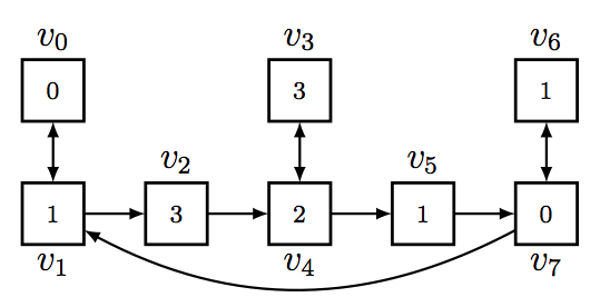
Figure 6: A 1-player parity game modified by neither psol, psolB nor psolQ.

5 Properties of our partial solvers

We already proved that our partial solvers are sound. Now we want to investigate additional properties of these partial solvers, looking first at their computational complexity.

5.1 Computational Complexity

We record that the partial solvers we designed above all run in polynomial time in the size of their input game.

Theorem 5

Let $G$ be a parity game with node set $V$, edge set $E$, and ${\mid\!{c}\!\mid}$ the number of its different colors.

1. The running time for partial solvers psol and psolB is in $O({{\mid\!{V}\!\mid}}^{2}\cdot{\mid\!{E}\!\mid})$.

2. The partial solvers psol and psolB can be implemented to run in time $O({{\mid\!{V}\!\mid}}^{3})$.

3. The partial solver psolQ runs in time $O({{\mid\!{V}\!\mid}}^{2}\!\cdot\!{\mid\!{E}\!\mid}\!\cdot\!{\mid\!{c}\!\mid})$.

Proof:

1. To see that the running time for psol is in $O({{\mid\!{V}\!\mid}}^{2}\cdot{\mid\!{E}\!\mid})$, note that all nodes have at least one successor in $G$ and so ${\mid\!{V}\!\mid}\leq{\mid\!{E}\!\mid}$. The computation of the attractor ${\mathsf{MA}({k})}$ in linear in the number of edges and so in $O({\mid\!{E}\!\mid})$. Each call of psol will compute at most ${\mid\!{V}\!\mid}$ many such attractors. In the worst case, there are ${\mid\!{V}\!\mid}$ many recursive calls. In summary, the running time is bound by $O({\mid\!{E}\!\mid}\cdot{\mid\!{V}\!\mid}\cdot{\mid\!{V}\!\mid})$ as claimed.

   To see that psolB also has running time in $O({{\mid\!{V}\!\mid}}^{2}\cdot{\mid\!{E}\!\mid})$, recall that we may compute ${\mathsf{MA}({X})}$ in time linear in ${\mid\!{E}\!\mid}$. Second, node set $V$ is partitioned into sets of nodes of a specific color, and so psolB can do at most ${\mid\!{V}\!\mid}$ many computations within the body of psolB before and if a recursive call happens.

2. The claim that psol and psolB can be implemented to run in $O({{\mid\!{V}\!\mid}}^{3})$ essentially reduces to showing that we can, in linear time, transform and reduce each computation of ${\mathsf{MA}({X})}$ to the solution of a Buchi game. This is so since Buchi games can be solved in time $O({{\mid\!{V}\!\mid}}^{2})$, as shown in [CH12]. Indeed, let $c$ denote $c(X)$, $p$ denote $p(X)$, and let $G[{\geq}c]$ denote the game obtained from $G$ by doing the following in the prescribed order.

   1. Remove from $G$ all nodes of color less than $c$, as well as all of their incoming and outgoing edges.

   2. Add to $G$ a sink node that has a self loop.

   3. Every node in $V_{p}$ not removed in the first step but where all of its successors were removed gets an edge to the new sink node.

   4. Every node in $V_{1-p}$ not removed in the first step but that had one of its successors removed gets an edge to the new sink node as well.

   5. If $p=1$, then we swap ownership of all remaining nodes: player $0$ nodes become player $1$ nodes, and vice versa.

   6. Finally, we color every node in $X$ by $0$ and all other nodes (including the new sink state) by $1$.

   It is possible to show that the winning region in $G[{\geq}c]$ is ${\mathsf{MA}({X})}$. Indeed, every node in the winning region of $G[{\geq}c]$ can be attracted to $X$ without passing through colors smaller than $c$ infinitely often. In the other direction, the attractor strategy to $X$ induced by ${\mathsf{MA}({X})}$ can be converted to a winning strategy in $G[{\geq}c]$. The size of $G[{\geq}c]$ is bounded by the size of $G$: there is at most one more node (the sink state), and each edge added to $G[{\geq}c]$ has a corresponding edge that is removed from $G$.

3. As before, the computation of layeredAttr($G,p,X$) can be completed in $O({\mid\!{V}\!\mid}\cdot{\mid\!{E}\!\mid})$. Indeed, the entire run of the for loop can be implemented so that each edge is crossed exactly once in all the monotone control predecessor computations. Then, the loop on $X$ and the loop on $b$ can run at most ${\mid\!{V}\!\mid}\cdot{\mid\!{c}\!\mid}$ times. And the number of times psolQ is called is bounded by ${\mid\!{V}\!\mid}$.

$\blacksquare$

If ${\tt psolQ}$ were to restrict attention to the last two iterations of the for loop, i.e., those that compute the greatest fixed-point with the maximal even color and the maximal odd color, the run time of ${\tt psolQ}$ would be bounded by $O({{\mid\!{V}\!\mid}}^{2}\cdot{\mid\!{E}\!\mid})$. For such a version of psolQ we also ran experiments on our benchmarks and do not report these results, except to say that this version performs considerably worse than psolQ in practice. We believe that this is so since psolQ more quickly discovers small winning regions that “destabilize” the rest of the games.

5.2 Robustness of psolB

Our pseudo-code for psolB iterates through colors in descending order. A natural question is whether the computed output game depends on the order in which these colors are iterated. Notice, that for psolQ there is no such dependency. Below, we formally state that the outcome of psolB – the residual parity game and the two sets ${{\mathsf{Win}}_{{{\tt psolB}}}[{G},{p}]}$ – is indeed independent of the iteration order. This suggests that the partial solver psolB computes a form of polynomial-time projection of parity games onto sub-games.

Let us formalize this. Let $\pi$ be some sequence of colors in $G$, that may omit or repeat some colors from $G$. Let ${\tt psolB}(\pi)$ be a version of psolB that checks for (and removes) fatal attractors according to the order in $\pi$ (including color repetitions in $\pi$). We say that ${\tt psolB}(\pi)$ is stable if for every color $c_{1}$, the input/output behavior of ${\tt psolB}(\pi)$ and ${\tt psolB}(\pi\cdot c_{1})$ are the same. That is, the sequence $\pi$ leads psolB to stabilization in the sense that every extension of the version ${\tt psolB}(\pi)$ with one color does not change the input/output behavior.

Theorem 6

Let $\pi_{1}$ and $\pi_{2}$ be sequences of colors with ${\tt psolB}(\pi_{1})$ and ${\tt psolB}(\pi_{2})$ stable. Then $G_{1}$ equals $G_{2}$ if $G_{i}$ is the output of ${\tt psolB}(\pi_{i})$ on $G$, for $1\leq i\leq 2$.

In order to prove Theorem 6 we first prove a few auxiliary lemmas. Below, we write $G[U]$ for the subgame identified by node set $U$.

Lemma 2

For every game $G$, for every set of nodes $K$ and for every trap $U$ for player $p$, the following holds: ${{\mathsf{Attr}}_{{p}}[{G},{K}]}\cap U\subseteq{{\mathsf{Attr}}_{{p}}[{G[U]},{K\cap U}]}$

Proof: The proof proceeds by induction on the distance from $K$ in ${{\mathsf{Attr}}_{{p}}[{G},{K}]}$. For every node $v$ of $G$ let $d(v)$ denote the distance of $v$ from $K$ in the attraction to $K$ in $G$.

• Suppose that $K\cap U=\emptyset$. Then, ${{\mathsf{Attr}}_{{p}}[{G[U]},{K\cap U}]}=\emptyset$ and we have to show that ${{\mathsf{Attr}}_{{p}}[{G},{K}]}\cap U=\emptyset$.

  Assume otherwise, then $v\in{{\mathsf{Attr}}_{{p}}[{G},{K}]}\cap U\neq\emptyset$. Let $v$ be the node of minimal distance to $K$ in ${{\mathsf{Attr}}_{{p}}[{G},{K}]}\cap U$. If $v\in V_{p}$, then there is some successor $w$ of $v$ such that $d(v)=d(w)+1$. However, $w$ cannot be in ${{\mathsf{Attr}}_{{p}}[{G},{K}]}\cap U$ by minimality of $v$. Thus, there is an edge from $v$ that leads to a node not in $U$ contradicting that $U$ is a trap for player $p$. Similarly, if $v\in V_{1-p}$, then for all successors $w$ of $v$ we have $d(v)>d(w)$ and it follows that all successors $w$ of $v$ are not in ${{\mathsf{Attr}}_{{p}}[{G},{K}]}\cap U$. So all successors of $v$ are not in $U$ and $U$ cannot be a trap for player $p$.

  It follows that ${{\mathsf{Attr}}_{{p}}[{G},{K}]}\cap U=\emptyset$ as required.

• Suppose that $K\cap U\neq\emptyset$. We prove that for every node $v\in{{\mathsf{Attr}}_{{p}}[{G},{K}]}\cap U$ we have $d_{G}(v,K)\geq d_{G[U]}(v,K\cap U)$, where $d_{G}(v,K)$ and $d_{G[U]}(v,K\cap U)$ are the distances of $v$ from $K$ (respectively $K\cap U$) in the computation of the corresponding attractor.

  Again, the proof proceeds by induction on $d_{G}(v,K)$. Consider a node $v$ in ${{\mathsf{Attr}}_{{p}}[{G},{K}]}\cap U$ such that $d_{G}(v,K)=0$. Then $v$ is in $K$ and from $v\in U$ we conclude that $v$ is in $K\cap U$ and $d_{G[U]}(v,K\cap U)=0$.

  Consider a node $v$ in ${{\mathsf{Attr}}_{{p}}[{G},{K}]}\cap U$ such that $d_{G}(v,K)>0$. If $v$ is in $V_{p}$, then there is a node $w$ such that $d_{G}(v,K)=d_{G}(w,K)+1$. Since $U$ is a trap, it must be the case that $w$ is in $U$ as well and hence $w$ is in ${{\mathsf{Attr}}_{{p}}[{G},{K}]}\cap U$. By induction $d_{G}(w,K)\geq d_{G[U]}(w,K\cap U)$.

  If $v$ is in $V_{1-p}$, then for all successors $w$ of $v$ we have $d_{G}(v,K)\geq d_{G}(w,K)+1$. Furthermore by $U$ being a trap, there is some successor $w$ of $v$ such that $w$ is in $U$. It follows that $w$ is in ${{\mathsf{Attr}}_{{p}}[{G},{K}]}\cap U$.

  As $U$ is a subset of the nodes of $G$ we have $succ(v,G)\supseteq succ(v,G[U])$, where $succ(v,G)$ is the set of successors of $v$ in $G$ and $succ(v,G[U])$ is the set of successors of $v$ in $G[U]$. But then, for every $w$ in $succ(v,G[U])$ we have $d_{G[U]}(w,K\cap U)\leq d_{G}(w,K)$. Hence, $d_{G[U]}(v,K\cap U)\leq d_{G}(v,K)$.

$\blacksquare$

We now specialize the above to the case of monotone attractors. We narrow the scope in this context to match its usage in ${\tt psolB}$. A more general claim talking about general sets in the spirit of Lemma 2 requires quite cumbersome notations and we skip it here (as it is not needed below).

Lemma 3

Consider a game $G$ and a set of nodes $K$ of color $c$ such that $p=c\%2$. For every trap $U$ for player $p$, the following holds: ${{{{\mathsf{MAttr}}}}_{p}({K},{c})}\cap U$ computed in $G$ is a subset of ${{{{\mathsf{MAttr}}}}_{p}({K\cap U},{c})}$ computed in $G[U]$.

Proof: The proof is very similar to the proof of Lemma 2 and proceeds by induction on the distance from $K$ in ${{{{\mathsf{MAttr}}}}_{p}({K},{c})}$. For every node $v$ of $G$ let $d(v)$ denote the distance of $v$ from $K$ in the monotone attraction to target $K$ in $G$.

• Suppose that $K\cap U=\emptyset$. Then, ${{{{\mathsf{MAttr}}}}_{p}({K\cap U},{c})}$ in $G[U]$ is empty and we have to show that ${{{{\mathsf{MAttr}}}}_{p}({K},{c})}$ in $G$ has empty intersection with $U$.

  Assume otherwise, then there is some $v$ such that $v$ is in ${{{{\mathsf{MAttr}}}}_{p}({K},{c})}$ in $G$ and $v\in U$. Let $v$ in $U$ be the node of minimal distance to $K$ in ${{{{\mathsf{MAttr}}}}_{p}({K},{c})}$ computed in $G$. If $d(v)=1$ and $v\in V_{p}$, then $v$ has some node in $K$ as successor. But $K\cap U=\emptyset$ and $v$ has a successor outside $U$ contradicting that $U$ is a trap. If $d(v)=1$ and $v$ is in $V_{1-p}$, then all successors of $v$ are in $K$. As $K\cap U=\emptyset$ all successors of $v$ are outside $U$ contradicting that $U$ is a trap. If $d(v)>1$, the case is similar. If $v$ is in $V_{p}$, then there is some successor $w$ of $v$ such that $d(v)=d(w)+1$. However, $w$ cannot be in ${{{{\mathsf{MAttr}}}}_{p}({K},{c})}\cap U$ computed in $G$, by the minimality of $v$. Thus, there is an edge from $v$ that leads to a node not in $U$ contradicting that $U$ is a trap for player $p$. Similarly, if $v$ is in $V_{1-p}$, then for all successors $w$ of $v$ we have $d(v)>d(w)$ and it follows that all successors $w$ of $v$ are not in ${{{{\mathsf{MAttr}}}}_{p}({K},{c})}\cap U$ in $G$. So all successors of $v$ are not in $U$ and $U$ cannot be a trap for player $p$.

  It follows that ${{{{\mathsf{MAttr}}}}_{p}({K},{c})}$ computed in $G$ does not intersect $U$ as required.

• Suppose that $K\cap U\neq\emptyset$. We prove that for every node $v$ in ${{{{\mathsf{MAttr}}}}_{p}({K},{c})}\cap U$ computed in $G$ we have $d_{G}(v,K)\geq d_{G[U]}(v,K\cap U)$, where $d_{G}(v,K)$ and $d_{G[U]}(v,K\cap U)$ are the distances of $v$ from $K$ (respectively $K\cap U$) in the computation of the corresponding monotone attractors.

  Again, the proof proceeds by induction on $d_{G}(v,K)$. Consider a node $v$ in ${{{{\mathsf{MAttr}}}}_{p}({K},{c})}$ computed in $G$ such that $v$ is in $U$ and $d_{G}(v,K)=1$. Then, if $v$ is in $V_{p}$, then $v$ has a successor in $K$. As $U$ is a trap, it must be the case that this successor is also in $U$ showing that $d_{G[U]}(v,K\cap U)=1$. If $v$ is in $V_{1-p}$, then all of $v$’s successors are in $K$. As $U$ is a trap, $v$ must have some successors in $G[U]$. It follows that $d_{G[U]}(v,K\cap U)=1$.

  Consider a node in ${{{{\mathsf{MAttr}}}}_{p}({K},{c})}$ such that $v$ is in $U$ and $d_{G}(v,K)>1$. If $v$ is in $V_{p}$ then there is a node $w$ such that $d_{G}(v,K)=d_{G}(w,K)+1$. By $U$ being a trap, it must be the case that $w$ is in $U$ as well and hence $w$ is in ${{{{\mathsf{MAttr}}}}_{p}({K},{c})}\cap U$ computed in $G$. By induction $d_{G}(w,K)\geq d_{G[U]}(w,K\cap U)$.

  If $v$ is in $V_{1-p}$, then for all successors $w$ of $v$ we have $d_{G}(v,K)\geq d_{G}(w,K)+1$. Furthermore by $U$ being a trap, there is some $w$ successor of $v$ such that $w$ is in $U$. It follows that all such $w$ are in ${{{{\mathsf{MAttr}}}}_{p}({K},{c})}\cap U$ computed in $G$.

  As $U$ is a subset of the nodes of $G$, we have $succ(v,G)\supseteq succ(v,G[U])$, where $succ(v,G)$ is the set of successors of $v$ in $G$ and $succ(v,G[U])$ is the set of successors of $v$ in $G[U]$. But then, for every $w$ in $succ(v,G[U])$ we have $d_{G[U]}(w,K\cap U)\leq d_{G}(w,K)$. Hence, $d_{G[U]}(v,K\cap U)\leq d_{G}(v,K)$.

$\blacksquare$

We now show that the order of removal of attractors for even and odd colors are interchangeable.

Lemma 4

Removal of fatal attractors for even colors and for odd colors are interchangeable.

Proof: Let $c_{1}$ be some odd color and $c_{0}$ be some even color. Let $X_{1}$ be the set of nodes of color $c_{1}$ such that $X_{1}\subseteq{{{{\mathsf{MAttr}}}}_{1}({X_{1}},{c_{1}})}$ and $X_{1}$ is the maximal node set with this property. (That is to say, $X_{1}$ is the set computed by a call to psolB with the color $c_{1}$.) Similarly, let $X_{0}$ be the set of nodes of color $c_{0}$ such that $X_{0}\subseteq{{{{\mathsf{MAttr}}}}_{0}({X_{0}},{c_{0}})}$ and $X_{0}$ is the maximal with this property. We assume that both ${{{{\mathsf{MAttr}}}}_{1}({X_{1}},{c_{1}})}$ and ${{{{\mathsf{MAttr}}}}_{0}({X_{1}},{c_{1}})}$ are not empty.

By soundness, ${{{{\mathsf{MAttr}}}}_{1}({X_{1}},{c_{1}})}$ is part of the winning region for player 1. Let $U$ be the residual game $G\setminus{{\mathsf{Attr}}_{{1}}[{G},{{{{{\mathsf{MAttr}}}}_{1}({X_{1}},{c_{1}})}}]}$. We note that Lemma 2 does not help us directly. Indeed, node set ${{\mathsf{Attr}}_{{1}}[{G},{{{{{\mathsf{MAttr}}}}_{1}({X_{1}},{c_{1}})}}]}$ is an attractor for player 1. Hence, $U$ is a trap for player 1 but not necessarily for player 0.

By soundness, ${{{{\mathsf{MAttr}}}}_{0}({X_{0}},{c_{0}})}$ is a subset of $U$. Indeed, all the nodes that are removed from $G$ are winning for player 1 but ${{{{\mathsf{MAttr}}}}_{0}({X_{0}},{c_{0}})}$ is part of the winning region for player 0. It follows that $X_{0}$ is a subset of $U$.

Furthermore, ${{{{\mathsf{MAttr}}}}_{0}({X_{0}\cap U},{c_{0}})}$ is a superset of ${{{{\mathsf{MAttr}}}}_{0}({X_{0}},{c_{0}})}$, where this follows from an argument similar to the one made in the proof of Lemma 2 above.

But from the construction of ${{{{\mathsf{MAttr}}}}_{0}({X_{0}\cap U},{c_{0}})}$ it follows that node set ${{{{\mathsf{MAttr}}}}_{0}({X_{0}\cap U},{c_{0}})}$ is also a subset of ${{{{\mathsf{MAttr}}}}_{0}({X_{0}},{c_{0}})}$. Indeed, if we consider the entire doubly nested fixpoint, then the computation of ${{{{\mathsf{MAttr}}}}_{0}({X_{0}\cap U},{c_{0}})}$ starts from a subset of the nodes of color $c_{0}$ and ${{{{\mathsf{MAttr}}}}_{0}({X_{0}},{c_{0}})}$ starts from the entire set of nodes of color $c_{0}$. $\blacksquare$

It follows that we may think about the removal of (attractors of) fatal attractors separately for all the even colors and all the odd colors. We now have all the tools in place to prove Theorem 6:

Proof: [of Theorem 6] By Lemma 4, we may assume that in both $\pi_{1}$ and $\pi_{2}$ all even colors occur before odd colors. We show that the node set of the output of version ${\tt psolB}(\pi_{1}\cdot\pi_{2})$ is a subset of the node set of the output of version ${\tt psolB}(\pi_{2})$. As $\pi_{1}$ is stable, it follows that actually ${\tt psolB}(\pi_{1})\subseteq{\tt psolB}(\pi_{2})$. The same argument works in the other direction and it follows that the two residual games are actually equivalent.

Let $\pi_{1}=c^{1}_{1}\cdots c^{1}_{n}$, where $c^{1}_{1},\ldots,c^{1}_{m}$ are even and $c^{1}_{m+1},\ldots,c^{1}_{n}$ are odd. Let $G^{1}_{0}$, $G^{1}_{1}$, $\ldots$, $G^{1}_{n}$ be the sequence of games after the different applications of the colors in $\pi_{1}$. That is, $G^{1}_{0}=G$, and $G^{1}_{i}$ is the result of applying psolB with color $c^{1}_{i}$ on $G^{1}_{i-1}$. It follows that $G^{1}_{n}=G_{1}$. Similarly, let $\pi_{2}=c^{2}_{1}\cdots c^{2}_{p}$, where $c^{2}_{1},\ldots,c^{2}_{q}$ are even and $c^{2}_{q+1},\ldots,c^{2}_{p}$ are odd. Let $G^{2}_{0}=G$ and let $G^{2}_{i}$ be the result of applying psolB with color $c^{2}_{i}$ on $G^{2}_{i-1}$. Let $G^{1,2}_{0}=G^{1}_{n}$ and $G^{1,2}_{i}$ is the result of applying psolB with color $c^{2}_{i}$ on $G^{1,2}_{i-1}$. We show that $G^{1,2}_{j}$ is a subset of $G^{2}_{j}$.

By Lemma 4 it is clear that we can consider the application of $c^{2}_{1},\ldots,c^{2}_{q}$ right after the application of $c^{1}_{1},\ldots,c^{1}_{m}$. Indeed, in the sequence $c^{1}_{m+1},\ldots,c^{1}_{n}$ is interchangeable with $c^{2}_{1},\ldots,c^{2}_{q}$.

Consider the application of $c^{2}_{j}$ to $G^{1,2}_{j-1}$ and to $G^{2}_{j-1}$. By induction $G^{1,2}_{j-1}$ is a subset of $G^{2}_{j-1}$. Furthermore, $G^{1,2}_{j-1}$ is obtained from $G$ by removing a sequence of attractors for player 0. It follows that $G^{1,2}_{j-1}$ is $G^{2}_{j-1}$ restricted to a trap for player 0.

It follows from Lemmas 3 and 2 that the computation of the attractor removes a larger part of $G^{1,2}_{j-1}$ than that of $G^{2}_{j-1}$. Hence $G^{1,2}_{j}$ is a subset of $G^{2}_{j}$. $\blacksquare$

5.3 Complete sub-classes for psolB

Next, we formally define classes of parity games, those that psolB solves completely and those that psolB does not modify. We concentrate on psolB as it seems to offer the best trade off between efficiency and discovery (see Section 6).

Definition 8

We define class ${\mathcal{S}}$ (for “Solved”) to consist of those parity games $G$ for which ${\tt psolB}(G)$ outputs the empty game. And we define ${\mathcal{K}}$ (for “Kernel”) as the class of those parity games $G$ for which ${\tt psolB}(G)$ outputs $G$ again.

The meaning of psolB is therefore a total, idempotent function of type ${\mathcal{P}G}\to{\mathcal{K}}$ that has ${\mathcal{S}}$ as inverse image of the empty parity game. By virtue of Theorem 6, classes ${\mathcal{S}}$ and ${\mathcal{K}}$ are semantic in nature.

We now show that ${\mathcal{S}}$ contains the class of Büchi games, which we identify with parity games $G$ with color $0$ and $1$ and where nodes with color $0$ are those that player $0$ wants to reach infinitely often.

Theorem 7

Let $G$ be a parity game whose colors are only $0$ and $1$. Then $G$ is in ${\mathcal{S}}$, i.e. psolB completely solves $G$.

Proof: We recall one way of solving a Büchi game, which takes the perspective of player $0$. First we inductively define, for $n\geq 0$, and $X=\{v\in V\mid c(v)=0\}$ the sets

$$Z^{0} = V\qquad\qquad\ \ U^{n}={{\mathsf{Attr}}_{{0}}[{G},{Z^{n}}]}$$ (6)

$$Z^{n+1} = Y^{n}\cap X\qquad Y^{n}={\mathsf{cpre}_{0}({U^{n}})}$$

Let $n_{0}$ be minimal such that $Z^{n_{0}}=Z^{n_{0}+1}$. The winning region for $W_{0}$ for player $0$ in game $G$ with colors $0$ and $1$ only is then equal to

$$W_{0}={{\mathsf{Attr}}_{{0}}[{G},{Z^{n_{0}}}]}$$ (7)

Since the order of processing colors in psolB does not impact its output game (by Theorem 6), we may assume that color $d=0$ gets processed first (this is just for convenience of presentation).

When the first iteration of psolB does process $d=0$, the computation essentially captures the process defined in the equations (6): the interplay of $U^{n}$ and $Y^{n}$ achieves the effect that player $0$ can move from $Y^{n}$ into $U^{n}$, which models that player $0$ can reach the target set again from every node in the target set. The computation of $Z^{n+1}$ corresponds to the else branch of the iteration within psolB. The constraint of our monotone attractor, that $c(v)\geq d$, is vacuously true here as $d$ equals $0$. So the first iteration will effectively compute set $Z^{n_{0}}$ as fixed-point. Then psolB will be called recursively on $G\setminus W_{0}$ by the definition of $W_{0}$ in (7).

In that remaining game, player $1$ can secure that all plays visit nodes of color $0$ only finitely often. This follows from the fact that $W_{0}$ was removed from game $G$ and that Büchi games are determined. In particular, psolB will not detect a fatal attractor for $d=0$ in that remaining game. But when its iteration runs with $d=1$ we argue as follows.

The following algorithm computes the winning region for player 1 in a Büchi game. Let $X=\{v\in V\mid c(v)=1\}$.

$$Z^{0} = \emptyset\qquad\qquad\qquad\qquad\ \ Y^{n,0}=X$$ (8)

$$Z^{n} = {{\mathsf{Attr}}_{{1}}[{G},{Y^{n,m^{n}_{0}}}]}\qquad Y^{n,m}=X\cap{\mathsf{cpre}_{1}({Z^{n-1}\cup Y^{n,m-1}})}$$

where $m^{n}_{0}$ is the minimal natural number such that $Y^{n,m^{n}_{0}}$ equals $Y^{n,m^{n}_{0}+1}$. Let $n_{0}$ be the minimal natural number such that $Z^{n_{0}}$ equals $Z^{n_{0}+1}$. Let $X^{i,j}$ denote the sequence of values computed for the variable $X$ in psolB, where $i$ is the number of recursive invocations of psolB, and $j$ is the value of $X$ computed after running in the loop $j$ times.

It is simple to see that $X^{n,m}$ is a superset of $Y^{n,m}$ restricted to the residual game in the $n$th call to psolB. Indeed, both start from the set $X$ and the computation of $X\cap{\mathsf{cpre}_{1}({Z^{n-1}\cup Y^{n,m-1}})}$ is contained in the computation of ${\mathsf{MA}({X^{n,m-1}})}$. The intersection with $X$ in the algorithm above is included in the definition of ${\mathsf{MA}({X})}$. Furthermore, every recursive call to psolB computes the exact attractor ${{\mathsf{Attr}}_{{1}}[{G},{{\mathsf{MA}({X})}}]}$ just as above. And the removal of nodes in psolB is equivalent to the inclusion of $Z^{n-1}$ in the computation of ${\mathsf{cpre}_{1}({Z^{n-1}\cup Y^{n,m-1}})}$. $\blacksquare$

There is interest in the computational complexity of specify types of parity games: do they have bespoke solvers that run in polynomial time, or are they solved in polynomial time by specific general solvers of parity games? Dittmann et al. [DKT12] prove that restricted classes of digraph parity games can be solved in polynomial time. Berwanger and Grädel prove such polynomial run-time complexities for weak and dull parity games [BG04]. Gazda and Willemse study the behavior of Zielonka’s algorithm for weak, dull, and solitaire games and adjust Zielonka’s algorithm to solve all three classes of parity games in polynomial time [GW13].

It is therefore of interest to examine whether ${\mathcal{S}}$ contains such classes of parity games. For example, not all 1-player parity games are in ${\mathcal{S}}$ (see Figure 6). Since the parity game in Figure 6 is also a dull [BG04] game, we infer that not all dull games are in ${\mathcal{S}}$ either. Class ${\mathcal{S}}$ is also not closed under sub-games, as the next example shows.

Example 7

Consider the game $G$ that is obtained from the one in Figure 1 by adding an edge from $v_{7}$ to $v_{3}$. Then psolB solves this game completely as there is now also a fatal attractor for $k=17$. But the game in Figure 1 is a sub-game of this game whose subset of nodes $\{v_{3},v_{5},v_{7}\}$ is not solved by psolB – as discussed in Example 1.

We recall that a parity game $G$ is deterministic if for all its nodes $v$, set $v.E$ has size $1$. We record that psolB solves completely all deterministic games – the proof of this fact easily can be modified to prove the corresponding fact for the partial solvers psol and psolQ.

Lemma 5

Let $G$ be a deterministic parity game. Then psolB solves $G$ completely.

Proof: Let $v$ be a node in $G$. Since $G$ is deterministic, there is exactly one play in $G$ beginning in $v$. This play has form $w_{1}w_{2}^{\omega}$ for finite words $w_{1}$ and $w_{2}$ over set $V$ and is won by player $k\%2$ where $k$ is defined to be $\min\{c(v^{\prime})\mid v^{\prime}\in w_{2}\}$. Let $v^{\prime}$ be in $w_{2}$ with $c(v^{\prime})=k$. Then the monotone attractor for $k$ in $G$ will contain at least $v^{\prime}$ and so the set $X$ of nodes of color $k$ in this attractor is non-empty. This means that ${\mathsf{MA}({X})}$ is a fatal attractor attractor that will be detected by psolB – by virtue of Theorem 6. Since $v$ is in ${{\mathsf{Attr}}_{{k\%2}}[{G},{X}]}$, we see that psolB decides the winner of node $v$ in $G$. $\blacksquare$

Finally, psolB solves all parity games that are weak in the sense of [BG04]. Weak parity games $G=(V,V_{0},V_{1},E,c)$ satisfy that for all edges $(v,w)$ in $E$ we have $c(v)\leq c(w)$. These games correspond to model-checking problems for the alternation-free fragment of the modal mu-calculus. The fact that colors increase along edges means that each maximal strongly connected component of the game graph $(V,E)$ has to have constant color, although different components may have different colors. We show that psolB solves such games completely.

Theorem 8

Let $G$ be a parity game such that for each of its maximal strongly connected components $C$ there is some color $c$ such that $c(v)=c$ for all $v$ in $C$. Then psolB completely solves $G$.

Proof: Let $G$ be such a game and consider the decomposition of $(V,E)$ into maximal strongly connected components (SCCs). The set of these SCCs is a partial order with $C\leq C^{\prime}$ iff there is some $(v,w)$ in $E\cap C\times C^{\prime}$. By Theorem 6, we may schedule the exploration of colors in the execution of psolB on $G$ in every possible order without changing the output. Let $c$ be a color of an SCC that is maximal in the partial order on SCCs. Then psolB will detect a fatal attractor for $c$ that contains $C$, and so $C$ (and possibly other nodes and edges) will be removed from $G$. Next, psolB will call itself recursively on this smaller game. Since psolB only removes normal game attractors before making such recursive calls, we know that the remaining game also satisfies the assumptions of this theorem. Therefore, after we applied a new SCC decomposition on that smaller game, we may again chose a color from some maximal SCC that will give rise to a fatal attractor. Thus, psolB solves $G$ completely after at most ${\mid\!{V}\!\mid}$ many recursive calls. $\blacksquare$

6 Experimental results

6.1 Experimental setup

We wrote Scala implementations of psol, psolB, and psolQ, and of Zielonka’s solver [Zie98] (zlka) that rely on the same data structures and do not compute winning strategies – which has routine administrative overhead. The (parity) Game object has a map of Nodes (objects) with node identifiers (integers) as the keys. Apart from colors and owner type (0 or 1), each Node has two lists of identifiers, one for successors and one for predecessors in the game graph $(V,E)$. For attractor computation, the predecessor list is used to perform “backward” attraction.

This uniform use of data types allows for a first informed evaluation. We chose zlka as a reference implementation since it seems to work well in practice on many games [FL09]. We then compared the performance of these implementations on all eight non-random, structured game types produced by the PGSolver tool [FL10]. Here is a list of brief descriptions of these game types.

• Clique: fully connected games with alternating colors and no self-loops.

• Ladder: layers of node pairs with connections between adjacent layers.

• Recursive Ladder: layers of $5$-node blocks with loops.

• Strategy Impr: worst cases for strategy improvement solvers.

• Model Checker Ladder: layers of $4$-node blocks.

• Tower Of Hanoi: captures well-known puzzle.

• Elevator Verification: a verification problem for an elevator model.

• Jurdzinski: worst cases for small progress measure solvers.

The first seven types take as game parameter a natural number $n$ as input, whereas Jurdzinski takes a pair of such numbers $n,m$ as game parameter.

For regression testing, we verified for all tested games that the winning regions of psol, psolB, psolQ and zlka  are consistent with those computed by PGSolver. Runs of these algorithms that took longer than 20 minutes (i.e. 1200K milliseconds) or for which the machine exhausted the available memory during solver computation are recorded as aborts (“abo”) – the most frequent reason for abo was that the used machine ran out of memory. The experiments on structured games were conducted on a machine with an Intel^® Core™ i5 (four cores) CPU at 3.20GHz and 8G of RAM, running on a Ubuntu 11.04 Linux operating system. The random part (Section 6.5) and precision tuning part (Section 7.2) of the experiments were conducted at a later stage, the test server used has two Intel^® E5 CPUs, with 6-core each running at 2.5GHz and 48G of RAM.

For most game types, we used unbounded binary search starting with $2$ and then iteratively doubling that value, in order to determine the abo boundary value for parameter $n$ within an accuracy of plus/minus $10$. As the game type Jurdzinski[$n,m$] has two parameters, we conducted three unbounded binary searches here: one where $n$ is fixed at $10$, another where $m$ is fixed at $10$, and a third one where $n$ equals $m$. We used a larger parameter configuration ($10$ $\times$ power of two) for Jurdzinski games.

We report here only the last two powers of two for which one of the partial solvers didn’t timeout, as well as the boundary values for each solver. For game types whose boundary value was less than $10$ (Tower Of Hanoi and Elevator Verification), we didn’t use binary search but incremented $n$ by $1$. Finally, if a partial solver didn’t solve its input game completely, we ran zlka on the remaining game and added the observed running times for zlka to that of the partial solver. (This occurred for Elevator Verification for psol and psolB.)

6.2 Experiments on structured games

Our experimental results are depicted in Figures 7–9, colored green (respectively red) for the partial solver with best (respectively worst) result. Running times are reported in milliseconds. The most important outcome is that partial solvers psol and psolB solved seven of the eight game types completely for all runs that did not time out, the exception being Elevator Verification; and that psolQ solved all eight game types completely. This suggests that partial solvers can actually be used as solvers on a range of structured game types.

Clique[$n$]                            $n$ psol psolB psolQ zlka 2**11 6016.68 48691.72 3281.57 12862.92 2**12 abo 164126.06 28122.96 76427.44 20min ${\color[rgb]{1,0,0}n=3680}$ ${\color[rgb]{0,1,0}n=5232}$ $n=4608$ $n=5104$

Ladder[$n$]            $n$ psol psolB psolQ zlka 2**19 abo 22440.57 26759.85 24406.79 2**20 abo 47139.96 59238.77 75270.74 20min ${\color[rgb]{1,0,0}n=14712}$ ${\color[rgb]{0,1,0}n=1596624}$ $n=1415776$ $n=1242376$

Model Checker Ladder[$n$]   $n$ psol psolB psolQ zlka 2**12 119291.99 90366.80 117006.17 79284.72 2**13 560002.68 457049.22 644225.37 398592.74 20min $n=11528$ $n=12288$ ${\color[rgb]{1,0,0}n=10928}$ ${\color[rgb]{0,1,0}n=13248}$

Recursive Ladder[$n$]   $n$ psol psolB psolQ zlka 2**12 abo abo 138956.08 abo 2**13 abo abo 606868.31 abo 20min $n=1560$ $n=2064$ ${\color[rgb]{0,1,0}n=11352}$ ${\color[rgb]{1,0,0}n=32}$

Figure 7: First experimental results for partial solvers run over benchmarks

Strategy Impr[$n$]                          $n$ psol psolB psolQ zlka 2**10 174913.85 134795.46 abo abo 2**11 909401.03 631963.68 abo abo 20min $n=2368$ ${\color[rgb]{0,1,0}n=2672}$ $n=40$ ${\color[rgb]{1,0,0}n=24}$

Tower Of Hanoi[$n$]              $n$ psol psolB psolQ zlka 9 272095.32 54543.31 610264.18 56780.41 10 abo 397728.33 abo 390407.41 20min ${\color[rgb]{1,0,0}n=9}$ ${\color[rgb]{0,1,0}n=10}$ ${\color[rgb]{1,0,0}n=9}$ ${\color[rgb]{0,1,0}n=10}$

Elevator Verification[$n$]   $n$ psol psolB psolQ zlka 1 171.63 120.59 147.32 125.41 2 646.18 248.56 385.56 237.51 3 2707.09 584.83 806.28 512.72 4 223829.69 1389.10 2882.14 1116.85 5 abo 11681.02 22532.75 3671.04 6 abo 168217.65 373568.85 41344.03 7 abo abo abo 458938.13 20min ${\color[rgb]{1,0,0}n=4}$ $n=6$ $n=6$ ${\color[rgb]{0,1,0}n=7}$

Figure 8: Second experimental results for partial solvers run over benchmarks

Jurdzinski[$10,m$]    $m$ psol psolB psolQ zlka 10x2**7 abo 179097.35 abo abo 10x2**8 abo 833509.48 abo abo 20min $n=560$ ${\color[rgb]{0,1,0}n=2890}$ $n=1120$ ${\color[rgb]{1,0,0}n=480}$

Jurdzinski[$n,10$]    $n$ psol psolB psolQ zlka 2**7x10 308033.94 106453.86 abo abo 2**8x10 abo 406621.65 abo abo 20min $n=2420$ ${\color[rgb]{0,1,0}n=4380}$ $n=1240$ ${\color[rgb]{1,0,0}n=140}$

Jurdzinski[$n,n$]         $n$ psol psolB psolQ zlka 2**3x10 215118.70 23045.37 310665.53 abo 2**4x10 abo 403844.56 abo abo 20min $n=110$ ${\color[rgb]{0,1,0}n=200}$ $n=100$ ${\color[rgb]{1,0,0}n=50}$

Figure 9: Third experimental results run over Jurdzinski benchmarks

We now compare the performance of these partial solvers and of zlka. There were ten experiments, three for Jurdzinski and one for each of the remaining seven game types.

For seven out of these ten experiments, psolB had the largest boundary value of the parameter and so seems to perform best overall. The solver zlka was best for Model Checker Ladder and Elevator Verification, and about as good as psolB for Tower Of Hanoi. And psolQ was best for Recursive Ladder. Thus psol appears to perform worst across these benchmarks.

Solvers psolB and zlka seem to do about equally well for game types Clique, Ladder, Model Checker Ladder, and Tower Of Hanoi. But solver psolB appears to outperform zlka dramatically for game types Recursive Ladder, and Strategy Impr and is considerably better than zlka for game type Jurdzinski.

We think these results are encouraging and corroborate that partial solvers based on fatal attractors may be components of faster solvers for parity games.

6.3 Number of detected fatal attractors

We also recorded the number of fatal attractors that were detected in runs of our partial solvers. One reason for doing this is to see whether game types have a typical number of dynamically detected fatal attractors that result in the complete solving of these games.

We report these findings for psol and psolB first: for Clique, Ladder, and Strategy Impr these games are solved by detecting two fatal attractors only; Model Checker Ladder was solved by detecting one fatal attractor. For the other game types psol and psolB behaved differently. For Recursive Ladder[$n$], psolB requires $n=2^{k}$ fatal attractors whereas psolQ needs only $2^{k-2}$ fatal attractors. For Jurdzinski[$n,m$], psolB detects $mn+1$ many fatal attractors, and psol removes $x$ edges where $x$ is about $nm/2\leq x\leq nm$, and detects slightly more than these $x$ fatal attractors. Finally, for Tower Of Hanoi[$n$], psol requires the detection of $3^{n}$ fatal attractors whereas psolB solves these games with detecting two fatal attractors only.

We also counted the number of recursive calls for psolQ: it equals the number of fatal attractors detected by psolB for all game types except Recursive Ladder, where it is $2^{k-1}$ when $n$ equals $2^{k}$.

6.4 Experiments on variants of partial solvers

We performed additional experiments on variants of these partial solvers. Here, we report results and insights on two such variants. The first variant is one that modifies the definition of the monotone control predecessor to

$${{{\mathsf{mpre}}}_{p}({A},{X},{c})} = \{v\in V_{p}\mid((c(v)\%2=p)\lor c(v)\geq c)\land v.E\cap(A\cup X)\neq\emptyset\}\cup$$

$$\{v\in V_{1-p}\mid((c(v)\%2=p)\lor c(v)\geq c)\land v.E\subseteq A\cup X\}$$

The change is that the constraint $c(v)\geq c$ is weakened to a disjunction $(c(v)\%2=p)\lor(c(v)\geq c)$ so that it suffices if the color at node $v$ has parity $p$ even though it may be smaller than $c$. This implicitly changes the definition of the monotone attractor and so of all partial solvers that make use of this attractor; and it also impacts the computation of $A$ within psolQ. Yet, this change did not have a dramatic effect on our partial solvers. On our benchmarks, the change improved things slightly for psol and made it slightly worse for psolB and psolQ.

A second variant we studied was a version of psol that removes at most one edge in each iteration (as opposed to all edges as stated in Fig. 2). For games of type Ladder, e.g., this variant did much worse. But for game types Model Checker Ladder and Strategy Impr, this variant did much better. The partial solvers based on such variants and their combination are such that psolB (as defined in Figure 3) is still better across all benchmarks.

6.5 Experiments on random games

With psolB having the best overall behavior over the structured games, we proceed to check its behavior over random games. It is our belief that comparing the behavior of parity game solvers on random games does not give an impression of how these solvers perform on parity games in practice. However, evaluating how often psolB completely solves random games complements the insight gained above that it completely solves many structured types of games. The experiment we conducted for this evaluation generated $100{,}000$ games with the randomgame command of PGSolver for each of $16$ different configurations, rendering a total of $1.6$ million games for that experiment. All of these games had $500$ nodes and no self-loops. A configuration had two parameters: a pair $(l,u)$ of minimal out-degree $l$ and maximal out-degree $u$ for all nodes in the game (ranging over $(1,5)$, $(5,10)$, $(50,250)$, and $(1,100)$ and where the out-degree for each node is chosen at random within the integer interval $[l,u]$), and a bound $c$ on the number of colors in the game (ranging over $500$, $250$, $50$, and $5$ and where colors at nodes are chosen at random).

This gave us $4\cdot 4=16$ configurations for random games on which we ran psolB. The results are shown in Figure 10. From the results in that figure we see that the behavior of psolB was similar across the four different color bounds for each of the four out-degree pairs $(l,u)$. For sake of brevity, we therefore only discuss here its behavior in terms of those out-degree pairs. Our results show that psolB did not solve completely only $4{,}534$ of all $1.6$ million random games ($99.9972\%$ solved completely). Breaking this down further, we see that when the edge density is low, with out-degree pair $(1,5)$, psolB did not solve completely only $4{,}529$ of the corresponding $400{,}000$ random games ($99.9887\%$ solved completely). The percentage of completely solved games increased to $99.9999875\%$ for the $400{,}000$ games with out-degree pair $(5,10)$ as only $5$ of these games were then not solved completely. For the remaining $800{,}000$ games, those with out-degree pairs $(50,250)$ or $(1,100)$, all were completely solved by psolB, i.e. it solved $100$% of those games. The average psolB run-time over these $1.6$ million games was $22$ms.

$c$	$(l,u)$	# nonempty	runtime
500	(1,5)	1086	22.56
250	(1,5)	1138	21.04
50	(1,5)	1030	20.79
5	(1,5)	1275	21.40
500	(5,10)	2	13.08
250	(5,10)	2	13.21
50	(5,10)	1	12.93
5	(5,10)	0	14.72

$c$	$(l,u)$	# nonempty	runtime
500	(50,250)	0	38.63
250	(50,250)	0	39.07
50	(50,250)	0	41.35
5	(50,250)	0	37.15
500	(1,100)	0	17.04
250	(1,100)	0	17.01
50	(1,100)	0	17.69
5	(1,100)	0	23.69

Figure 10: Experimental results for psolB. Each row shows for $100{,}000$ random games $G$ with color bound $c$ and out-degree pair $(l,u)$: how often psolB did not solve games completely (# nonempty), and average running times in milliseconds of psolB. All but $4{,}534$ of these $1.6$ million games were solved completely

7 Tuning the precision of partial solvers

So far, we constructed partial solvers that result from variants of monotone attractor definitions and that simply remove such attractors whenever they are fatal. We now suggest another principle for building partial solvers, one that takes a partial solver as input and outputs another partial solver that may increase the precision of its input solver. As before, we concentrate on psolB as it seems to offer the best balance of performance and accuracy.

7.1 Partial solver transformation ${\mathsf{lift}}$

We fix notation for removing choices from a parity game:

Definition 9

Let $G=(V,V_{0},V_{1},E,c)$ be a parity game and $e=(v,w)$ an edge in $E$.

1. Parity game $G_{e}$ equals $(V,V_{0},V_{1},E^{\prime},c)$ with $E^{\prime}=\{(v^{\prime},w^{\prime})\in E\mid v^{\prime}\not=v\hbox{ or }w^{\prime}=w\}$.

2. Parity game $G\setminus e$ equals $(V,V_{0},V_{1},E\setminus\{e\},c)$.

Game $G_{e}$ is obtained from game $G$ by selecting an edge in $G$ and then removing all edges from the source of $e$ that do not point to its target node. This makes the game deterministic at the source node of $e$. And game $G\setminus e$ simply removes edge $e$ from $G$. We next introduce formal properties of partial solvers that are useful for reasoning about the transformation of partial solvers that we will define below.

Definition 10

Let ${\mathsf{\rho}}$ be a partial solver.

1. Soundness: ${\mathsf{\rho}}$ is sound if for all games $G$ all nodes in ${{\mathsf{Win}}_{{{\mathsf{\rho}}}}[{G},{0}]}$ are won by player $0$ in $G$, and all nodes in ${{\mathsf{Win}}_{{{\mathsf{\rho}}}}[{G},{1}]}$ are won by player $1$ in $G$.

2. Idempotency: ${\mathsf{\rho}}$ is idempotent if for all games $G$ as input game, the output games for ${\mathsf{\rho}}$ and the sequential composition of ${\mathsf{\rho}}$ with itself are equal: $\rho(G)=\rho(\rho(G))$.

3. Locality: ${\mathsf{\rho}}$ is local if for all games $G$, all players $p$ in $\{0,1\}$, and all edges $e=(v,w)$ in $G$ with $v$ in $V_{p}$ we have that ${{\mathsf{Win}}_{{{\mathsf{\rho}}}}[{G},{1-p}]}=\emptyset$ and ${{\mathsf{Win}}_{{{\mathsf{\rho}}}}[{G_{e}},{1-p}]}\not=\emptyset$ imply $v\in{{\mathsf{Win}}_{{{\mathsf{\rho}}}}[{G_{e}},{1-p}]}$.

The property Locality considers scenarios in which partial solver $\rho$ cannot decide winning nodes for player $1-p$ in game $G$, but where $\rho$ can decide winning nodes for player $1-p$ in $G$ after we restrict node $v$ in $V_{p}$ to have $w$ as only successor in the game graph. In such scenarios, locality of $\rho$ means that $\rho$ then also decides node $v$ to be won by player $1-p$ in the restricted game $G_{(v,w)}$. This behavior is expected, for example, when a partial solver decides winning nodes through a variant of attractor computations as studied in this paper. We formally prove that psolB satisfies these properties.

Lemma 6

Partial solver psolB satisfies Soundness, Idempotency, and Locality.

Proof: Soundness of psolB has been shown in Theorem 3. Idempotency follows from Theorem 6. We now show Locality. Let $G$, $p$, and $e=(v,w)$ in $E_{G}$ be given with $v\in V_{p}$ such that ${{\mathsf{Win}}_{{{\tt psolB}}}[{G},{1-p}]}=\emptyset$ and ${{\mathsf{Win}}_{{{\tt psolB}}}[{G_{e}},{1-p}]}\not=\emptyset$. Proof by contradiction: Assume that $v$ is not in ${{\mathsf{Win}}_{{{\tt psolB}}}[{G_{e}},{1-p}]}$. Then $w$ also cannot be in ${{\mathsf{Win}}_{{{\tt psolB}}}[{G_{e}},{1-p}]}$ since $v.E_{G_{e}}=\{w\}$ and since ${{\mathsf{Win}}_{{{\tt psolB}}}[{G_{e}},{1-p}]}$ is a $1-p$ attractor in game $G_{e}$ by definition of psolB. But then neither $v$, nor $w$, nor the edge $(v,w)$ can be part of a fatal attractor discovered in ${{\mathsf{Win}}_{{{\tt psolB}}}[{G_{e}},{1-p}]}$. From ${{\mathsf{Win}}_{{{\tt psolB}}}[{G_{e}},{1-p}]}\not=\emptyset$ we know that the run ${\tt psolB}(G_{e})$ discovers at least one such fatal attractor. But since neither $v$ nor $w$ are contained in it, this would also be a fatal attractor in $G$, contradicting that ${{\mathsf{Win}}_{{{\tt psolB}}}[{G},{1-p}]}=\emptyset$. $\blacksquare$

We now describe a transformation of partial solvers that is sound for partial solvers that satisfy the above properties. Pseudo-code for our transformation of partial solvers is depicted in Figure 11. Function ${\mathsf{lift}}$ takes a partial solver ${\mathsf{\rho}}$ as input and outputs another partial solver ${\mathsf{lift}}({\mathsf{\rho}})$. The pseudo-code describes the behavior of ${\mathsf{lift}}({\mathsf{\rho}})$ on a parity game $G$.

The partial solver ${\mathsf{lift}}({\mathsf{\rho}})$ first applies partial solver ${\mathsf{\rho}}$ to game $G$ and resets $G$ to the sub-game of $G$ of nodes that ${\mathsf{\rho}}$ did not decide to be won by some player. Next, an iteration starts over all nodes of the remaining game that have out-degree $>1$. For such a node $v$, we record the owner of $v$ in $p$. We then cache in $W$ the value of node set $v.E$ and start an iteration over that node set $W$. In each such iteration, we use ${\mathsf{\rho}}$ to compute a winning region of player $1-p$ in game $G_{(v,w)}$. If that region is non-empty, we call ${\mathsf{lift}}({\mathsf{\rho}})$ recursively on the game $G\setminus(v,w)$. The intuition for this is that, by fixing the edge $(v,w)$ as the strategy of player $p$ from node $v$ in $V_{p}$ makes player $p$ lose plays from that node. Therefore, it is safe to remove edge $(v,w)$ from the game without limiting the ability of player $p$ to win node $v$.

${\mathsf{lift}}$(${\mathsf{\rho}}$)($G$) {
l1:   $G$ = ${\mathsf{\rho}}$($G$);
l2:   for ($v\in\!\!V$ with outdegree $>1$) {
l3:       $p$ = owner($v$);
l4:       $W$ = $v.E$;
l5:       for ($w\in\!\!W$) {
l6:           if ($\mathsf{}{Win}_{{\mathsf{\rho}}}(G_{(v,w)},\!\!1-p)$ != $\emptyset$) { return ${\mathsf{lift}}({\mathsf{\rho}})(G\setminus\!\!(v,w))$; }
l7:       }
l8:   }
l9:   return $G$;
}

Figure 11: Pseudo-code of a transformation that takes a partial solver ${\mathsf{\rho}}$ of parity games as input and returns another partial solver.

We emphasize that ${\mathsf{lift}}({\mathsf{\rho}})$ does not directly detect winning nodes, it merely removes edges. Rather, the detection of winning nodes is done by ${\mathsf{\rho}}$ itself at program point ${\tt l1}$. We illustrate this with an example.

Example 8

Reconsider the parity game $G$ in Figure 6 and the following execution of ${\mathsf{lift}}({\tt psolB})(G)$: the initial assignment to $G$ won’t change $G$ as psolB cannot detect winning nodes in $G$. Suppose that the execution first picks $v$ to be $v_{4}$ and chooses as first $w$ node $v_{3}$. Then both $v_{3}$ and $v_{4}$ are contained in ${{\mathsf{Win}}_{{{\tt psolB}}}[{G_{(v_{4},v_{3})}},{0}]}$, which is therefore non-empty. The execution therefore removes edge $(v_{4},v_{3})$ from $G$, calls psolB on the resulting game, and assigns its output to $G$. But that output is the empty game since the removed edge make the nodes of color $0$ a fatal attractor for that color. We conclude that ${\mathsf{lift}}({\tt psolB})$ solves this game completely.

We now analyze the computational overhead of ${\mathsf{lift}}$ when called with a partial solver ${\mathsf{\rho}}$, and prove that ${\mathsf{lift}}({\mathsf{\rho}})$ is sound for partial solvers ${\mathsf{\rho}}$ that satisfy the above formal properties.

Theorem 9

Let ${\mathsf{\rho}}$ be a sound partial solver. Then we have the following:

1. If partial solver ${\mathsf{\rho}}$ satisfies Soundness, Itempotency, and Locality then ${\mathsf{lift}}({\mathsf{\rho}})$ satisfies Soundness.

2. The computational time complexity of ${\mathsf{lift}}({\mathsf{\rho}})$ is in $O(({\mid\!{E}\!\mid}-{\mid\!{V}\!\mid})^{2}\cdot{\mid\!{{\mathsf{\rho}}}\!\mid}))$ where ${\mid\!{{\mathsf{\rho}}}\!\mid}$ is the computational time complexity of partial solver ${\mathsf{\rho}}$. In particular, ${\mathsf{lift}}({\mathsf{\rho}})$ runs in polynomial time if ${\mathsf{\rho}}$ does.

Proof: Let $\rho$ be a partial solver that satisfies these properties. Let $G$ be a parity game.

1. Consider the run of ${\mathsf{lift}}({\mathsf{\rho}})(G)$. Each execution of its body removes a (possibly empty) node set $X_{i}$ from the game at program point ${\tt l1}$. If a recursive call happens (in the if-branch at program point ${\tt l6}$), this node removal event $X_{i}$ is then followed by the removal of an edge $e_{i}$ from the game. We can therefore capture essential state change information for such a run by a finite sequence

   $$X_{0},e_{0},X_{1},e_{1},\dots,X_{m-1},e_{m-1},X_{m}$$ (9)

   where the removal of node set $X_{m}$ results in a game that is the output of ${\mathsf{lift}}({\mathsf{\rho}})(G)$ (no more recursive calls occur thereafter). Since ${\mathsf{\rho}}$ satisfies Soundness, we can conclude that the decisions of winning nodes made implicitly by ${\mathsf{lift}}({\mathsf{\rho}})(G)$ in node sets $X_{i}$ are sound provided that the edge removals in the above sequence change neither winning regions nor the sets of winning strategies in these games. We formalize the latter notion now:

   Let $G$ and $G^{\prime}$ be parity games that have the same set of nodes and the same coloring function. We write $G\equiv G^{\prime}$ iff the winning regions of these parity games are equal and the sets of winning strategies of players, when restricted to their winning regions, are equal as well. So let $G$ be the state of the game in the run in (9) right before edge $e_{i}$ gets removed. And let $G^{\prime}$ be $G\setminus e_{i}$. It suffices to show that $G\equiv G^{\prime}$ since then all edge removals performed in (9) preserve winning regions and sets of winning strategies until the next set of nodes $X_{j}$ gets removed from the game. Soundness of ${\mathsf{\rho}}$ and the transitivity of $\equiv$ then guarantee that decisions made implicitly by the sound partial solver ${\mathsf{\rho}}$ in node set $X_{j}$ are sound as well.

   We now prove that $G\equiv G\setminus e_{i}$ where $e_{i}=(v,w)$ and $v$ in $V_{p}$. We do a case analysis over which player wins node $v$ in $G$:

   • Let $v$ be won by player $1-p$ in (the current state of) $G$. Since $v$ is owned by player $p$ and since $G^{\prime}$ equals $G\setminus(v,w)$ we infer $G\equiv G^{\prime}$: node $v$ is not in the winning region of player $p$ and so winning strategies of player $p$ won’t differ when restricted to the winning region of player $p$. Hence the sets of winning strategies for both players, restricted to their winning regions, are equal in $G$ and in $G^{\prime}$. And their winning regions are also equal since player $1-p$ wins node $v$ owned by player $p$ and so the edge chosen at $v$ affects the winning status of no nodes. So $G\equiv G^{\prime}$ follows.

   • Let $v$ be won by player $p$ in (the current state of) $G$. Let $\sigma$ be a winning strategy of player $p$ on her winning region in $G$. Then $\sigma(v)$ is defined on that winning region. Proof by contradiction: let $\sigma(v)=w$. Since $(v,w)$ gets removed from the current $G$ in this run, we know that

     $${{\mathsf{Win}}_{{{\tt psolB}}}[{G_{(v,w)}},{1-p}]}\not=\emptyset\hbox{ and }{{\mathsf{Win}}_{{{\tt psolB}}}[{G},{1-p}]}=\emptyset$$ (10)

     where the latter is true since program point ${\tt l1}$ got executed and since ${\mathsf{\rho}}$ satisfies Idempotency. Since ${\mathsf{\rho}}$ also satisfies Locality, we infer from (10) that $v$ is in ${{\mathsf{Win}}_{{{\tt psolB}}}[{G_{(v,w)}},{1-p}]}$. Since ${\mathsf{\rho}}$ satisfies Soundness, we conclude from this that $v$ is won by player $1-p$ in $G_{(v,w)}$. Since $\sigma(v)=w$ and $\sigma$ is a winning strategy for player $p$, we know that $G$ and $G_{(v,w)}$ have the same winning regions. Therefore, we know that $v$ is also won by player $1-p$ in game $G$. But this is a contradiction to this second case. Thus, we know that $\sigma(v)\not=w$. In particular, removing edge $(v,w)$ from $G$ won’t change the sets of winning regions of either player and it won’t change the sets of winning strategies for either player. So we showed that $G\equiv G^{\prime}$ holds.

   To summarize, we have shown that every sequence of edge removals $e_{i}\dots e_{i+k}$ with $k\geq 0$ for which all node sets $X_{i+1}$ up to $X_{i+k}$ are empty are such that $G\equiv G^{*}$ where $G$ is the game before the removal of $e_{i}$, and $G^{*}$ is the game after removal of $e_{i+k}$. As already discussed, this suffices to show that ${\mathsf{lift}}({\mathsf{\rho}})(G)$ is sound.

2. Let $G$ be an input parity game. Let $k$ be ${\mid\!{E}\!\mid}-{\mid\!{V}\!\mid}$. Since each node in $G$ has out-degree at least $1$, the value $k$ expresses an upper bound on the number of edges that can be removed from $G$ in ${\mathsf{lift}}({\mathsf{\rho}})$.

   • Let us analyze the complexity of the for-statement that ranges over $v\in U$: there is one initial call to ${\mathsf{\rho}}$ and at most $k$ many calls to ${\mathsf{\rho}}$ within these nested for-statements, and these calls are the dominating factor in that part of the code. Thus, an upper bound for the time complexity within these for-statements is $(k+1)\cdot{\mid\!{{\mathsf{\rho}}}\!\mid}$.

   • Now we turn to the question of how often ${\mathsf{lift}}({\mathsf{\rho}})$ may call itself. Each such call removes at least one edge from the input $G$ for the next call, and so there can be at most $k$ such calls.

   Combining this, we get as upper bound $k\cdot(k+1)\cdot{\mid\!{{\mathsf{\rho}}}\!\mid}$ which is in $O(k^{2}\cdot{\mid\!{{\mathsf{\rho}}}\!\mid})$.

$\blacksquare$

7.2 Experimental results for ${\mathsf{lift}}({\tt psolB})$

We now evaluate the effectiveness of ${\mathsf{lift}}$ on the partial solver psolB, where we are mostly interested in the increase of precision that ${\mathsf{lift}}({\tt psolB})$ has over psolB. We evaluated this over all structural parity game types used in earlier experiments and over the $1.6$ million randomly generated games. As before, we applied regression testing to confirm that all computed winning regions are consistent with the (full) winning regions computed by PGSolver.

For the data set of $1.6$ million randomly generated games, we ran ${\mathsf{lift}}({\tt psolB})$ on those $4{,}534$ games that psolB did not solve completely. Figure 12 shows the results we obtained. Let us first discuss the results for out-degree pair $(1,5)$. Partial solver ${\mathsf{lift}}({\tt psolB})$ completely solves $4{,}182$ of the $4{,}534$ games that psolB could not solve completely ($92.236\%$); in other words, it could not solve completely only $352$ of these $400{,}000$ random games. The last two columns in Figure 12 suggest that the run-time overhead of ${\mathsf{lift}}({\tt psolB})$ over psolB is proportional to the maximal number of recursive calls of ${\mathsf{lift}}({\tt psolB})$, i.e. to the maximal number of edge removals E_rem. We saw at most $31$ such recursive calls for these $500$ node games, and the values for N_sol are on average about half of the size of the node set ($500)$ of the input games.

For games of out-degree pair $(5,10)$ only five games were not solved completely by psolB and so only these five games were run with ${\mathsf{lift}}({\tt psolB})$ for that out-degree pair. It therefore make little sense to discuss edge and node removal and runtimes for such a small data set. However, we can see that ${\mathsf{lift}}({\tt psolB})$ completely solved all of these five games.

An additional result not shown in Figure 12 relates to games that are not solved completely by both psolB and ${\mathsf{lift}}({\tt psolB})$ – a total of $347$ out of $1.6$ million. On only four such games was ${\mathsf{lift}}({\tt psolB})$ able to solve additional nodes, on the remaining $343$ games ${\mathsf{lift}}({\tt psolB})$ had no effect over running psolB.

$c$	$(l,u)$	# games	# empty	E_rem	N_sol	runtime
500	(1,5)	1086	1051	16	225	126.90
250	(1,5)	1138	1102	22	224	150.59
50	(1,5)	1030	987	21	251	172.91
5	(1,5)	1275	1042	31	350	4905.58
500	(5,10)	2	2	1	4	19.57
250	(5,10)	2	2	1	3	19.48
50	(5,10)	1	1	1	3	22.33

Figure 12: Experimental results for ${\mathsf{lift}}({\tt psolB})$ for the seven configurations of Figure 10 in which psolB does not solve all games completely: how many games psolB could not solve completely (# games), how many of those games ${\mathsf{lift}}({\tt psolB})$ could solve completely (# empty), the maximal number of edges removed in a run of ${\mathsf{lift}}({\tt psolB})$ (E_rem), the maximum number of additional nodes solved by ${\mathsf{lift}}({\tt psolB})$ (N_sol), and the average running times in milliseconds of ${\mathsf{lift}}({\tt psolB})$

For the other data set with structured parity games, we ran ${\mathsf{lift}}({\tt psolB})$ only over games of type ${\tt Elevator\ Verification[n]}$, since this was the only structured game type that psolB did not solve completely in our experiments. In doing so, we determined that ${\mathsf{lift}}({\tt psolB})$ solves the same node sets that psolB solves, and so it also cannot solve such games completely. Therefore, we conclude that transformation ${\mathsf{lift}}$ is unable to deal with the stuttering inherent in these games when applied to psolB.

8 Conclusions

We proposed a new approach to studying the problem of solving parity games: partial solvers as polynomial algorithms that correctly decide the winning status of some nodes and return a sub-game of nodes for which such status cannot be decided. We demonstrated the feasibility of this approach both in theory and in practice. Theoretically, we developed a new form of attractor that naturally lends itself to the design of such partial solvers; and we proved results about the computational complexity and semantic properties of these partial solvers. Practically, we showed through extensive experiments that these partial solvers can compete with extant solvers on benchmarks – both in terms of practical running times and in terms of precision in that our partial solvers completely solve such benchmark games.

We then suggested that such partial solvers can be subjected to a transformation that increases their complexity within PTIME but also lets them solve more games completely. We studied such a concrete transformation and showed its soundness for partial solvers that satisfy reasonable conditions. We then proved that psolB meets these conditions and thoroughly evaluated the effect of this transformation on psolB over random games, demonstrating the potential of that transformation to increase the precision of partial solvers whilst still ensuring polynomial time running times.

In future work, we mean to study the descriptive complexity of the class of output games of a partial solver, for example of psolQ. We also want to research whether such output classes can be solved by algorithms that exploit invariants satisfied by these output classes; insights gained in such an investigation may lead to the design of full solvers that contain partial solvers as building blocks. Furthermore, we mean to investigate whether classes of games characterized by structural properties of their game graphs can be solved completely by partial solvers. Such insights may connect our work to that of [DKT12], where it is shown that certain classes of parity games that can be solved in PTIME are closed under operations such as the join of game graphs. Finally, we want to investigate whether and how partial solvers can be integrated into solver design patterns such as the one proposed in [FL09].

We refer to [HKP13b] for the initial conference paper reporting on this work, which neither contains proofs nor the material on transforming partial solvers. A technical report [HKP13a] accompanies the paper [HKP13b] and contains – amongst other things – selected proofs, the pseudo-code of our version of Zielonka’s algorithm, and further details on experimental results and their discussion. Transformations akin to ${\mathsf{lift}}$ have been suggested already in [HPW09] as a means of making preprocessors of parity games more effective.

References

- [BDHK06] Dietmar Berwanger, Anuj Dawar, Paul Hunter, and Stephan Kreutzer. Dag-width and parity games. In STACS, pages 524–536, 2006.
- [BE01] Olaf Burkart and Javier Esparza. More infinite results. In Current Trends in Theoretical Computer Science, pages 480–503. 2001.
- [BG04] Dietmar Berwanger and Erich Grädel. Fixed-point logics and solitaire games. Theory Comput. Syst., 37(6):675–694, 2004.
- [BG08] Antonio Bucchiarone and Juan P. Galeotti. Dynamic software architectures verification using dynalloy. ECEASST, 10, 2008.
- [Bla09] Bruno Blanchet. Automatic verification of correspondences for security protocols. Journal of Computer Security, 17(4):363–434, 2009.
- [BLR11] Thomas Ball, Vladimir Levin, and Sriram K. Rajamani. A decade of software model checking with slam. Commun. ACM, 54(7):68–76, 2011.
- [CE81] Edmund M. Clarke and E. Allen Emerson. Design and synthesis of synchronization skeletons using branching-time temporal logic. In Logic of Programs, pages 52–71, 1981.
- [CGJ+03] Edmund M. Clarke, Orna Grumberg, Somesh Jha, Yuan Lu, and Helmut Veith. Counterexample-guided abstraction refinement for symbolic model checking. J. ACM, 50(5):752–794, 2003.
- [CGL94] Edmund M. Clarke, Orna Grumberg, and David E. Long. Model checking and abstraction. ACM Trans. Program. Lang. Syst., 16(5):1512–1542, 1994.
- [CH12] Krishnendu Chatterjee and Monika Henzinger. An o(n) time algorithm for alternating büchi games. In SODA, pages 1386–1399, 2012.
- [DKT12] Christoph Dittmann, Stephan Kreutzer, and Alexandru I. Tomescu. Graph operations on parity games and polynomial-time algorithms. CoRR, abs/1208.1640, 2012.
- [EJ91] E. Allen Emerson and Charanjit S. Jutla. Tree automata, mu-calculus and determinacy (extended abstract). In FOCS, pages 368–377, 1991.
- [EJS93] E. Allen Emerson, Charanjit S. Jutla, and A. Prasad Sistla. On model-checking for fragments of -calculus. In CAV, pages 385–396, 1993.
- [FL09] Oliver Friedmann and Martin Lange. Solving parity games in practice. In ATVA, pages 182–196, 2009.
- [FL10] Oliver Friedmann and Martin Lange. The PGSolver Collection of Parity Game Solvers. Technical Report Version 3, Institut für Informatik, LMU Munich, 3 February 2010.
- [GW13] Maciej Gazda and Tim A. C. Willemse. Zielonka’s recursive algorithm: dull, weak and solitaire games and tighter bounds. In GandALF, pages 7–20, 2013.
- [HKP13a] Michael Huth, Jim Huan-Pu Kuo, and Nir Piterma. Fatal attractors in parity game. Technical Report 2013/1, Department of Computing, Imperial College London, January 2013.
- [HKP13b] Michael Huth, Jim Huan-Pu Kuo, and Nir Piterman. Fatal attractors in parity games. In FoSSaCS, pages 34–49, 2013.
- [HPW09] Michael Huth, Nir Piterman, and Huaxin Wang. A workbench for preprocessor design and evaluation: toward benchmarks for parity games. ECEASST, 23, 2009.
- [JPZ08] Marcin Jurdzinski, Mike Paterson, and Uri Zwick. A deterministic subexponential algorithm for solving parity games. SIAM J. Comput., 38(4):1519–1532, 2008.
- [Jur98] Marcin Jurdzinski. Deciding the winner in parity games is in up co-up. Inf. Process. Lett., 68(3):119–124, 1998.
- [Jur00] Marcin Jurdzinski. Small progress measures for solving parity games. In STACS, pages 290–301, 2000.
- [Koz83] Dexter Kozen. Results on the propositional mu-calculus. Theor. Comput. Sci., 27:333–354, 1983.
- [Mos91] Andrzej Wlodzimierz Mostowski. Games with forbidden positions. Technical Report 78, University of Gdańsk, 1991.
- [NNH99] Flemming Nielson, Hanne Riis Nielson, and Chris Hankin. Principles of program analysis. Springer, 1999.
- [QS82] Jean-Pierre Queille and Joseph Sifakis. Specification and verification of concurrent systems in cesar. In Symposium on Programming, pages 337–351, 1982.
- [Sti95] Colin Stirling. Local model checking games. In CONCUR, pages 1–11, 1995.
- [UABD+13] Sebastián Uchitel, Dalal Alrajeh, Shoham Ben-David, Víctor A. Braberman, Marsha Chechik, Guido de Caso, Nicolás D’Ippolito, Dario Fischbein, Diego Garbervetsky, Jeff Kramer, Alessandra Russo, and German E. Sibay. Supporting incremental behaviour model elaboration. Computer Science - R&D, 28(4):279–293, 2013.
- [VJ00] Jens Vöge and Marcin Jurdzinski. A discrete strategy improvement algorithm for solving parity games. In CAV, pages 202–215, 2000.
- [Zie98] Wieslaw Zielonka. Infinite games on finitely coloured graphs with applications to automata on infinite trees. Theor. Comput. Sci., 200(1-2):135–183, 1998.