Frequentist and Bayesian inference for Gaussian-log-Gaussian wavelet trees and statistical signal processing applications

Abstract

We introduce new estimation methods for a sub-class of the Gaussian scale mixture models for wavelet trees by Wainwright, Simoncelli & Willsky that rely on modern results for composite likelihoods and approximate Bayesian inference. Our methodology is illustrated for denoising and edge detection problems in two-dimensional images.

Key words: conditional auto-regression; EM algorithm; hidden Markov tree; integrated nested Laplace approximations.

1 Introduction

Statistical models of wavelet coefficients in signal processing aims at modelling their non-Gaussian nature and statistical dependencies. Different models have been proposed for this task, in particular a broad class of models for wavelet coefficients known as Gaussian scale mixtures [1, 13]. The present paper introduces new procedures for inference in a subclass of these models that we refer to as Gaussian-log-Gaussian wavelet tree models or just GLG models. Briefly, a GLG model specifies dependence in highpass wavelet coefficients with $d\geq 1$ directional subbands by a hidden Gaussian Markovian tree structure such that coefficients given the hidden states are independent and each coefficient follows a zero-mean Gaussian distribution with the log-variance equal to the corresponding hidden state. Further details of the GLG model are given in Section 2.

Section 3 introduces parameter estimation with moment matching and an expectation-maximization (EM) algorithm. The moment-based estimates can be used as initial values for the EM algorithm. The EM algorithm is based on composite likelihoods and is fast and accurate if $d=1$ or if we assume independence for hidden states corresponding to different directional subbands as is customary in many situations.

Section 4 demonstrates how the GLG model fits in the integrated nested Laplace approximation (INLA) framework [10, 11] for doing fast approximative Bayesian inference. In particular the marginal posterior distributions for the parameters can be estimated but the INLA approach requires a relatively low dimensional parameter as compared with the dimenionality of the parameter in the full GLG model. In a simulation study in Section 5 we compare the results of the INLA approach with the results of the EM algorithm.

As examples of applications Section 6 discusses how the GLG model can be used for denoising and edge detection in images.

Technical details are deferred to Appendices A-C . Matlab and R [9] codes for our statistical inference procedures are available at http://people.math.aau.dk/~robert/software.

2 The Gaussian-log-Gaussian wavelet tree model

This section recaps the GLG model [13] and sets the notation.

The wavelet transform of a signal is separated into lowpass and highpass coefficients. We wish to model the highpass coefficients, denoted $\mathbf{w}=(\bm{w}_{1},\ldots,\bm{w}_{n})$, with respect to a given directed tree, see Figure 1 for a simple example. Here $i=1,\ldots,n$ is an abstract index identified with the nodes of the tree, the root is $i=1$ (the coarsest level of the wavelet transform) and the directed edges correspond to the parent-child relations of the coefficients at the coarsest to the finest level. Specifically, we denote

• $r(i)$ the level of node $i$, that is, $r(i)$ is the number of nodes in the path from the root to $i$; thus $r(1)=1$;

• $L$ the number of levels (the longest path);

• $c(i)\subset\{1,\ldots,n\}$ the children of $i$, that is, there is a directed edge from $i$ to each child $j\in c(i)$; if $i$ is at the finest wavelet level, $i$ has no children ($c(i)=\emptyset$); else $c(i)\neq\emptyset$; in our image examples, $c(i)$ has cardinality 4 whenever $c(i)\not=\emptyset$; and for convenience we let $c(0)=\{1\}$;

• $\rho(j)$ the parent to node $j\neq 1$, that is, there is a directed edge from $\rho(j)$ to $j$.

Furthermore, each $\bm{w}_{i}=(w_{i}(1),\ldots,w_{i}(d))$ corresponds to $d\geq 1$ directional subbands, where $d$ depends on the dimension of the signal. In our examples with images, $d=3$.

Figure 1: Illustration of a binary tree structure corresponding to a one-dimensional signal (that is, $d=1$) with 3 levels of wavelet coefficients (that is, $L=3$). Node $j$ has one parent $\rho(j)$ and node $i$ has two children $c(i)$.

We model the dependence structure for the coefficients through hidden states as follows. Assume that each $\bm{w}_{i}$ has an associated hidden state $\bm{s}_{i}=(s_{i}(1),\ldots,s_{i}(d))$ such that conditional on all hidden states $\mathbf{s}=(\bm{s}_{1},\ldots,\bm{s}_{n})$, the coefficients $w_{i}(\ell)$ ($\ell=1,\ldots,d$, $i=1,\ldots,n$) are independent and the conditional distribution of $\bm{w}_{i}$ depends only on $\bm{s}_{i}$ and has density

$$p\bigl{(}\bm{w}_{i}\,|\,\bm{s}_{i}\bigr{)}\sim N_{d}\bigl{(}\bm{0},\operatorname{\text{diag}}\bigl{[}\exp(s_{i}(\ell)),\ell=1,\ldots,d\bigr{]}\bigr{)}.$$ (1)

Here $N_{d}$ denotes the $d$-dimensional Gaussian distribution and the covariance matrix in (1) is diagonal.

We consider a parametric graphical model for the hidden states, using $\bm{\theta}$ as generic notation for the unknown parameters appearing in (LABEL:eq:theta) later, and assume tying within levels as follows. Viewing $\mathbf{s}$ as a directed graphical model [6], we assume that the conditional independence structure for $\bm{s}_{1},\ldots,\bm{s}_{n}$ is given by the tree structure. Hence the joint density for coefficients and hidden states given $\bm{\theta}$ has the structure

$$p(\mathbf{w},\mathbf{s}\,|\,\bm{\theta})=p\bigl{(}\bm{s}_{1}\,|\,\bm{\mu}_{1},\bm{\Sigma}_{1}\bigr{)}\prod_{i=1}^{n}\Bigl{[}p(\bm{w}_{i}\,|\,\bm{s}_{i})\prod_{j\in c(i)}p\bigl{(}\bm{s}_{j}\,|\,\bm{s}_{i},\bm{\alpha}_{r(i)},\bm{B}_{r(i)},\bm{K}_{r(i)}\bigr{)}\Bigr{]},$$ (2)

where we set the product over the empty set to be $1$ and where we impose the conditional densities

$$p\bigl{(}\bm{s}_{1}\,|\,\bm{\mu}_{1},\bm{\Sigma}_{1}\bigr{)} \sim N_{d}\bigl{(}\bm{\mu}_{1},\bm{\Sigma}_{1}\bigr{)},$$ (3)

$$p\bigl{(}\bm{s}_{j}\,|\,\bm{s}_{i},\bm{\alpha}_{r(i)},\bm{B}_{r(i)},\bm{K}_{r(i)}\bigr{)} \sim N_{d}\bigl{(}\bm{\alpha}_{r(i)}+\bm{B}_{r(i)}\bm{s}_{i},\bm{K}_{r(i)}\bigr{)},$$ (4)

Thus $\bm{\theta}$ consists of the elements of the parameter vectors and matrices

$$\begin{split}&\bm{\mu}_{1}=[\mu_{1,\ell}]_{\ell=1,\ldots,d},\quad\bm{\Sigma}_{1}=\bigl{[}\sigma_{1,\ell,\ell^{\prime}}\bigr{]}_{\ell,\ell^{\prime}=1,\ldots,d},\\ &\bm{\alpha}_{r}=[\alpha_{r,\ell}]_{\ell=1,\ldots,d},\quad\bm{K}_{r}=\bigl{[}\kappa_{r,\ell,\ell^{\prime}}\bigr{]}_{\ell,\ell^{\prime}=1,\ldots,d},\quad\bm{B}_{r}=\bigl{[}\beta_{r,\ell,\ell^{\prime}}\bigr{]}_{\ell,\ell^{\prime}=1,\ldots,d},\end{split}$$ (5)

with $r=1,\ldots,L-1$.

We call (2) the (full) GLG (GLG) model if we add no further restrictions than $\bm{\mu}_{1}$ and $\bm{\alpha}_{r}$ being real $d$-dimensional vectors, $\bm{B}_{r}$ being a real $d\times d$ matrix, and $\bm{\Sigma}_{1}$ and $\bm{K}_{r}$ being symmetric and strictly positive definite $d\times d$ matrices. The submodel where the matrices $\bm{\Sigma}_{1}$, $\bm{K}_{1},\ldots,\bm{K}_{L-1}$ and $\bm{B}_{1},\ldots,\bm{B}_{L-1}$ are diagonal is called the directional independence GLG model, because hidden variables corresponding to different directional subbands are independent. We also consider the simpler homogenous GLG model where for all $\ell=1,\ldots,d$ and $r=1,\ldots,L-1$,

$$\mu_{1,\ell}=\mu_{1},\quad\bm{\Sigma}_{1}=\sigma_{1}\bm{I}_{d},\quad\alpha_{r,\ell}=\alpha,\quad\bm{K}_{r}=\kappa\bm{I}_{d},\quad\bm{B}_{r}=\beta\bm{I}_{d},$$

where $\bm{I}_{d}$ is the $d\times d$ identity matrix and $\mu_{1}\in\mathbb{R}$, $\sigma_{1}>0$, $\alpha\in\mathbb{R}$, $\kappa>0$ and $\beta\in\mathbb{R}$ are the five free parameters. The number of free parameters in the full GLG model is $d+d(d+1)(3L/2-1)$, that is, $18L-9$ if $d=3$. In the directional independence GLG model we have $d(2+3L)$ free parameters, that is, $9L+6$ if $d=3$.

The inference procedures introduced later will be based on $k\geq 1$ wavelet trees $\mathbf{w}^{(t)}=(\bm{w}_{1}^{(t)},\ldots,\bm{w}_{n}^{(t)})$, $t=1,\ldots,k$; in our examples, the pixels of an image correspond to the nodes of the $k$ trees after applying the (inverse) wavelet transform. We denote the corresponding hidden states by $\mathbf{s}^{(t)}=(\bm{s}_{1}^{(t)},\ldots,\bm{s}_{n}^{(t)})$, $t=1,\ldots,k$, and assume that $(\mathbf{w}^{(1)},\mathbf{s}^{(1)}),\ldots,\mathbf{w}^{(k)},\mathbf{s}^{(k)})$ are independent copies of $(\mathbf{w},\mathbf{s})$. We denote all the coefficients (our data) and all the hidden states by

$${\bar{\mathbf{w}}}=(\mathbf{w}^{(1)},\ldots,\mathbf{w}^{(k)}),\quad{\bar{\mathbf{s}}}=(\mathbf{s}^{(1)},\ldots,\mathbf{s}^{(k)}).$$

2.1 Mean and variance-covariance structure

We shall later exploit the following marginal distributions for the hidden states and the connection between their mean and variance-covariance structure and the original parametrization in (LABEL:eq:theta).

By (3) and (4), each hidden state $\bm{s}_{j}$ follows a $d$-dimensional Gaussian distribution with a mean vector and covariance matrix depending only on the level $r(j)$:

$$p\left(\bm{s}_{j}\ |\ \bm{\mu}_{r(j)},\bm{\Sigma}_{r(j)}\right)\sim N_{d}\left(\bm{\mu}_{r(j)},\bm{\Sigma}_{r(j)}\right)$$ (6)

where the mean vector and covariance matrix are determined recursively from the coarsest level to the second finest level by

$$\bm{\mu}_{r+1}=\bm{\alpha}_{r}+\bm{B}_{r}\bm{\mu}_{r},\quad\bm{\Sigma}_{r+1}=\bm{K}_{r}+\bm{B}_{r}\bm{\Sigma}_{r}\bm{B}_{r}^{\top},\quad r=1,\ldots,L-1,$$ (7)

where $\bm{B}_{r}^{\top}$ denotes the transpose of $\bm{B}_{r}$. For a node $i$ at level $r=r(i)$ and with children $j,h\in c(i)$, we obtain from (4) that

$$\operatorname{Cov}(\bm{s}_{j},\bm{s}_{i})=\bm{B}_{r}\bm{\Sigma}_{r},\quad\operatorname{Cov}(\bm{s}_{j},\bm{s}_{h})=\bm{B}_{r}\bm{\Sigma}_{r}\bm{B}_{r}^{\top}\quad\mbox{if $j\neq h$}.$$

3 Frequentist inference

This section introduces estimating equations based on moment relations and an EM algorithm. The main purpose of the moment method is to provide initial parameter estimates for the EM algorithm.

3.1 Moment matching relations

Moments of the form $\operatorname{E}\bigl{[}w_{i}(\ell)^{a}w_{j}(\ell^{\prime})^{b}\bigr{]}$ for $1\leq i,j\leq n$, $1\leq\ell,\ell^{\prime}\leq d$ and $a,b\in\{0,1,\ldots\}$ can be derived by conditioning on the hidden states and exploiting well-known moment results for the log-Gaussian distribution. Matching these expressions for the moments with empirical moments estimates allows us to estimate the parameters. The details are deferred to Appendix A.

3.2 Composite likelihoods and the EM algorithm

The EM algorithm in Section 3.2.2 is based on composite likelihoods and to this end we need the marginal distributions in Section 3.2.1.

3.2.1 Marginal distributions for wavelet coefficients

First, combining (1) and (3), we obtain the joint density at the root,

$$p(\bm{s}_{1},\bm{w}_{1}\,|\,\bm{\mu}_{1},\bm{\Sigma}_{1})=p(\bm{w}_{1}\,|\,\bm{s}_{1})p(\bm{s}_{1}\,|\,\bm{\mu}_{1},\bm{\Sigma}_{1})$$

$$=\frac{1}{(2\pi)^{d}\det(\bm{\Sigma}_{1})}\exp\biggl{(}-\frac{1}{2}\biggl{[}\biggl{\{}\sum_{\ell=1}^{d}\frac{w_{1}(\ell)^{2}}{\exp(s_{1}(\ell))}+s_{1}(\ell)\biggr{\}}+(\bm{s}_{1}-\bm{\mu}_{1})^{\top}\bm{\Sigma}_{1}^{-1}(\bm{s}_{1}-\bm{\mu}_{1})\biggr{]}\biggr{)}$$ (8)

and thereby the marginal density of the root wavelet,

$$p(\bm{w}_{1}\,|\,\bm{\mu}_{1},\bm{\Sigma}_{1})=\int_{\mathbb{R}^{d}}p(\bm{s}_{1},\bm{w}_{1}\,|\,\bm{\mu}_{1},\bm{\Sigma}_{1})\mathrm{d}\bm{s}_{1}.$$ (9)

Hence the marginal log-likelihood based on the root wavelets $\overline{\bm{w}}_{1}=(\bm{w}_{1}^{(1)},\ldots,\bm{w}_{1}^{(k)})$ for the $k$ trees is given by

$$l_{1}(\bm{\mu}_{1},\bm{\Sigma}_{1}|\overline{\bm{w}}_{1})=\sum_{t=1}^{k}\log p(\bm{w}_{1}^{(t)}\,|\,\bm{\mu}_{1},\bm{\Sigma}_{1}).$$ (10)

Second, consider any $i\in\{1,\ldots,n\}$ with level $r=r(i)<L$. Denote $\bm{w}_{i,c(i)}$ the vector consisting of $\bm{w}_{i}$ and all $\bm{w}_{j}$ with $j\in c(i)$, and $\bm{s}_{i,c(i)}$ the vector consisting of $\bm{s}_{i}$ and all $\bm{s}_{j}$ with $j\in c(i)$. Using (1), (4) and (6), we obtain the density of $\bigl{(}\bm{s}_{i,c(i)},\bm{w}_{i,c(i)}\bigr{)}$,

$$p(\bm{s}_{i,c(i)},\bm{w}_{i,c(i)}\,|\,\bm{\mu}_{r},\bm{\Sigma}_{r},\bm{\alpha}_{r},\bm{B}_{r},\bm{K}_{r})$$

$$={} p(\bm{w}_{i}\,|\,\bm{s}_{i})\ p(\bm{s}_{i}\,|\,\bm{\mu}_{r},\bm{\Sigma}_{r})\prod_{j\in c(i)}p(\bm{w}_{j}\,|\,\bm{s}_{j})\ p(\bm{s}_{j}\,|\,\bm{s}_{i},\bm{\alpha}_{r},\bm{B}_{r},\bm{K}_{r})$$

$$={} \frac{1}{(2\pi)^{d(1+|c(i)|)}\det(\bm{\Sigma}_{r})^{1/2}\det(\bm{K}_{r})^{|c(i)|/2}}$$

$$\exp\biggl{(}-\frac{1}{2}\biggl{[}\biggl{\{}\sum_{\ell=1}^{d}\frac{w_{i}(\ell)^{2}}{\exp(s_{i}(\ell))}+s_{i}(\ell)\biggr{\}}+(\bm{s}_{i}-\bm{\mu}_{r})^{\top}\bm{\Sigma}_{r}^{-1}(\bm{s}_{i}-\bm{\mu}_{r})$$

$$+\sum_{j\in c(i)}\biggl{\{}\sum_{\ell=1}^{d}\frac{w_{j}(\ell)^{2}}{\exp(s_{j}(\ell))}+s_{j}(\ell)\biggr{\}}+(\bm{s}_{j}-\bm{\alpha}_{r}-\bm{B}_{r}\bm{s}_{i})^{\top}\bm{K}_{r}^{-1}(\bm{s}_{j}-\bm{\alpha}_{r}-\bm{B}_{r}\bm{s}_{i})\biggr{]}\biggr{)},$$ (11)

where $|c(i)|$ denotes the number of children of node $i$, and so $\bm{w}_{i,c(i)}$ has density

$$p(\bm{w}_{i,c(i)}\,|\,\bm{\mu}_{r},\bm{\Sigma}_{r},\bm{\alpha}_{r},\bm{B}_{r},\bm{K}_{r})$$

$$=\int_{\mathbb{R}^{d(1+|c(i)|)}}p(\bm{s}_{i,c(i)},\bm{w}_{i,c(i)}\,|\,\bm{\mu}_{r-1},\bm{\Sigma}_{r-1},\bm{\alpha}_{r},\bm{B}_{r},\bm{K}_{r})\mathrm{d}\bm{s}_{i,c(i)}.$$ (12)

Hence, denoting $\overline{\bm{w}}_{i,c(i)}$ the vector of the $i$th wavelets $\bm{w}_{i}^{(1)},\ldots,\bm{w}_{i}^{(k)}$ and their children $\bm{w}_{j}^{(1)},\ldots,\bm{w}_{j}^{(k)}$, $j\in c(i)$, the log-likelihood based on $\overline{\bm{w}}_{i,c(i)}$ is

$$l_{r}(\bm{\mu}_{r},\bm{\Sigma}_{r},\bm{\alpha}_{r},\bm{B}_{r},\bm{K}_{r}\,|\,\overline{\bm{w}}_{i,c(i)})=\sum_{t=1}^{k}\sum_{j\in c(i)}p(\bm{w}_{r}^{(t)},\bm{w}_{j}^{(t)}\,|\,\bm{\mu}_{r},\bm{\Sigma}_{r},\bm{\alpha}_{r},\bm{B}_{r},\bm{K}_{r}).$$ (13)

A common thread in the integrals (9) and (12) is that (8) and (11) are of the form

$$\text{non-linear function}\times\text{Gaussian density}.$$

This suggests that the Gauss-Hermite quadrature rule is a good choice for evaluating the integral, see, for example, [8]. Indeed, under the directional independence GLG model or if $d=1$, this is fast and accurate. However, for the full GLG model with $d=3$, it is not feasible to calculate (12) to a reasonable precision with quadrature rules because of the large number of times it is required in the EM algorithm in the following section—even with sparse grids as used in, for example, [4].

3.2.2 The composite EM algorithm

Because the following EM algorithm applies on composite likelihoods [3] defined from the marginal likelihoods in Section 3.2.1, we call it the composite EM algorithm. In brief, it proceeds from the coarsest to the finest level, using the relation (7) for the parameters in the marginal and conditional distributions of the hidden variables as follows.

1. Apply the EM algorithm for the log-likelihood (10) to obtain an estimate $(\widehat{\bm{\mu}}_{1},\widehat{\bm{\Sigma}}_{1})$.

2. For $r=1,\ldots,L-1$ proceed as follows. Denote $\overline{\bm{w}}_{(r)}$ the vector of all $\overline{\bm{w}}_{i,c(i)}$ with $\ell(i)=r$. Note that the log-composite likelihood given by the sum of the log-likelihoods (13) based on all $\overline{\bm{w}}_{i,c(i)}$ with $\ell(i)=r$ is

   $$l_{r}(\bm{\mu}_{r},\bm{\Sigma}_{r},\bm{\alpha}_{r},\bm{B}_{r},\bm{K}_{r}\,|\,\overline{\bm{w}}_{(r)})=\sum_{i:\ell(i)=r}l_{i}(\bm{\mu}_{r},\bm{\Sigma}_{r},\bm{\alpha}_{r},\bm{B}_{r},\bm{K}_{r}\,|\,\overline{\bm{w}}_{i,c(i)}).$$

   Then, using a previously obtained estimate $(\widehat{\bm{\mu}}_{r},\widehat{\bm{\Sigma}}_{r})$, apply the EM algorithm on $l_{r}(\widehat{\bm{\mu}}_{r},\widehat{\bm{\Sigma}}_{r},\bm{\alpha}_{r},\bm{B}_{r},\bm{K}_{r}\,|\,\overline{\bm{w}}_{(r)})$ to obtain an estimate $(\widehat{\bm{\alpha}}_{r},\widehat{\bm{B}}_{r},\widehat{\bm{K}}_{r})$. Thereby, using (7), an estimate $(\widehat{\bm{\mu}}_{r+1},\widehat{\bm{\Sigma}}_{r+1})$ is also obtained.

Appendix B details these steps.

4 Bayesian inference

Section 4.1 provides a brief description of approximate Bayesian inference for our GLG model using integrated nested Laplace approximations. Section 5 compares the Bayesian approach with the EM algorithm of Section 3.2.2.

4.1 A short diversion into INLA

Integrated nested Laplace approximations (INLA) is a general framework for performing approximate Bayesian inference in latent Gaussian models. The INLA approach is described in [11, 7] and has been implemented in the R-INLA package that is publicly available from the homepage http://www.r-inla.org.

In fact the INLA approach applies for a wide range of latent Gaussian Markov random field models, including those considered in the present paper, where wavelet coefficients ${\bar{\mathbf{w}}}$ (the observations) are conditionally independent given the hidden states ${\bar{\mathbf{s}}}$ and the unknown parameters $\bm{\theta}$. Here we assume a directional independence GLG model for ${\bar{\mathbf{s}}}$. Furthermore, we need to impose a prior distribution on $\bm{\theta}$, where standard priors have been implemented in R-INLA package that also allows the user to specify his or her ‘own prior’.

INLA provides a recipe for fast Bayesian inference using accurate approximations to $p(\bm{\theta}|{\bar{\mathbf{w}}})$, that is, the marginal posterior density for the parameters, and to $p(s_{i}^{(t)}(\ell)|{\bar{\mathbf{w}}})$, that is, the marginal posterior density for each hidden state $i=1,\ldots,n$ of each tree $t=1,\ldots,k$ and each direction $\ell=1,\ldots,d$. Thereby we can calculate (approximate) posterior means and variances as well as other summaries of interest. The approximations are based on integrated nested Laplace approximations as detailed in [11, 7]. Because the approximations involve numerical integration with respect to $\bm{\theta}$, the dimension of $\bm{\theta}$ needs to be sufficiently small.

Compared to approximate Bayesian inference using Markov chain Monte Carlo methods, INLA is much faster and accurate, cf. [11].

5 Simulation study

To test and compare composite estimates based on the composite EM algorithm with inference based on INLA, we simulate wavelet coefficients from 100 images, each consisting of 256 wavelet trees with three levels, under a homogenous GLG model with parameter values

$$\mu_{1}=-1,\quad\sigma_{1}=1,\quad\alpha=-1,\quad\beta=1,\quad\kappa=1.$$ (14)

This implies that $\mu_{2}=-2$, $\mu_{3}=-3$, $\sigma_{2}^{2}=2$ and $\sigma_{3}^{2}=3$, compare with (7).

Table 1 shows the average parameter estimates and their standard deviations for estimation with the composite EM algorithm of section Section 3.2.2. The marginal parameters $\mu$ and $\sigma$ are well estimated, but the transition parameters are not estimated as well.

	$D=1$		$D=2$		$D=3$
$\mu_{1}$	$-0.976$	$(0.125$)	$-0.956$	$(0.136$)	$-0.941$	$(0.139$)
$\mu_{2}$	$-1.947$	$(0.175$)	$-1.953$	$(0.131$)	$-1.945$	$(0.179$)
$\mu_{3}$	$-2.956$	$(0.270$)	$-2.968$	$(0.209$)	$-2.952$	$(0.277$)
$\sigma_{1}$	$0.937$	$(0.291$)	$0.915$	$(0.284$)	$0.891$	$(0.275$)
$\sigma_{2}$	$1.843$	$(0.314$)	$1.847$	$(0.323$)	$1.813$	$(0.343$)
$\sigma_{3}$	$2.823$	$(0.429$)	$2.824$	$(0.435$)	$2.813$	$(0.460$)
$\alpha_{1}$	$-1.562$	$(0.332$)	$-1.662$	$(0.310$)	$-1.654$	$(0.360$)
$\alpha_{2}$	$-1.707$	$(0.340$)	$-1.748$	$(0.323$)	$-1.716$	$(0.325$)
$\beta_{1}$	$0.410$	$(0.328$)	$0.304$	$(0.284$)	$0.316$	$(0.325$)
$\beta_{2}$	$0.646$	$(0.124$)	$0.630$	$(0.148$)	$0.642$	$(0.125$)
$\kappa_{1}$	$1.664$	$(0.359$)	$1.711$	$(0.390$)	$1.669$	$(0.376$)
$\kappa_{2}$	$2.053$	$(0.485$)	$2.105$	$(0.496$)	$2.087$	$(0.472$)

Table 1: Results for parameter estimation based on 100 simulations under the homogenous GLG model with parameter values specified in (14) and obtained using the composite EM algorithm of Section 3.2.2. The $D$ refer to the directional subband. For each parameter the average of 100 parameter estimates is shown together with their standard deviation (show in in parantheses).

Table 2 summarizes the Bayesian inference with INLA. As a point estimate the marginal posterior mean for each parameter is calculated along with the standard deviation of the 100 estimates, that is,

$$\overline{\operatorname{E}(\theta\,|\,\bar{\bm{w}})}=\frac{1}{100}\sum_{n=1}^{N}\operatorname{E}(\theta\,|\,\bar{\bm{w}}_{n}),$$

$$\sqrt{\frac{1}{99}\sum_{n=1}^{N}\bigl{(}\operatorname{E}(\theta\,|\,\bar{\bm{w}}_{n})-\overline{\operatorname{E}(\theta\,|\,\bar{\bm{w}})}\bigr{)}^{2}},$$

where $\bar{\bm{w}}_{n}$ denotes the $n$’th simulated data set. Note that INLA does not work with variances, but with precisions; that is, we have access to the marginal posterior distributions of $\sigma^{-2}$ and $\kappa^{-2}$. The estimates in Table 2 are computed as the average of the inverse posterior means.

$\mu$		$\sigma$		$\alpha$		$\beta$		$\kappa$
$-0.45$	$(0.072$)	$0.010$	$(0.051$)	$-1.39$	$(0.065$)	$0.82$	$(0.052$)	$1.39$	$(0.074$)

Table 2: Results for parameter estimation based on 100 simulations under the homogenous GLG model with parameter values specified in (14) and obtained using the Bayesian approach of Section 4. For each parameter the average of 100 parameter estimates is shown together with their standard deviation (show in in parantheses).

To illustrate the advantages of the Bayesian approach Figure 2 shows the marginal posterior distributions for the parameters of a single simulation. Unlike the frequentist EM algorithm the Bayesian approach provides information about the uncertainty of the parameters. One particular thing to notice is the very non-localized distribution for $\sigma^{-2}$. In our experiments this seems to be a general issue for small data sets – for a large dataset this posterior distribution is much more localized, see Figure 3 for the posterior distribution of $\sigma^{-2}$ from the ’Lena’ image in Figure 4.

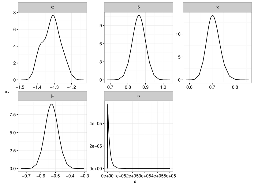
Figure 2: Marginal posterior distributions for each of the parameters in a single simulation. The distributions labellel “$\sigma$” and “$\kappa$” are actually the posterior distributions for $\sigma^{-2}$ and $\kappa^{-2}$, respectively.

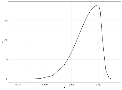
Figure 3: Posterior distribution of $\sigma^{-2}$ from the ’Lena’ image in Figure 4.

6 Examples of applications

This section demonstrates how the GLG model applies to denoising and edge detection in images. The examples are meant to illustrate different applications, not to make thorough comparisons with other methods. We use three test images from the USC-SIPI image database available at http://sipi.usc.edu/database: ’Lena’, ’mandrill’, and ’peppers’, see Figure 4. These images are 512-by-512 pixels represented as 8 bit grayscale with pixel values in the unit interval.

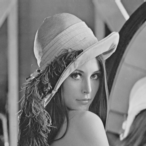
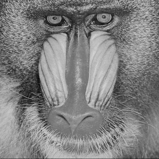
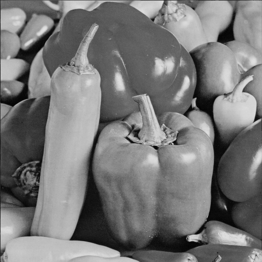
Figure 4: The three test images: ’Lena’, ’mandrill’, and ’peppers’.

6.1 Denoising

Consider an image corrupted with additive white noise, that is, we add independent terms to the pixel values from the same zero-mean normal distribution. Then the procedure for denoising with orthonormal wavelets works as follows

$$\text{noisy data}\to\text{noisy wavelets}\to\text{noise-free wavelets}\to\text{noise-free data}$$

where the distribution and the independence properties of the noise are preserved by the wavelet transform, so the problem of estimating noise-free data boils down to considering each wavelet tree observed with additive white noise:

$$v_{i}^{(t)}(\ell)=w_{i}^{(t)}(\ell)+\varepsilon_{i}^{(t)}(\ell),\quad\ell=1,\ldots,d,\ i=1,\dots,n,\ t=1,\ldots,k,$$ (15)

where the $\varepsilon_{i}^{(t)}(\ell)$ are mutually independent, identically $N(0,\sigma_{\varepsilon}^{2})$-distributed and independent of $({\bar{\mathbf{w}}},{\bar{\mathbf{s}}})$. The dependence structure in a tree with noisy observations is illustrated in Figure 5 (suppressing the dependence of the indices $t$ and $\ell$).

Figure 5: Graphical model of a binary tree with two levels and noisy observations. The rectangular nodes are observed variables and the round nodes are unobserved variables.

Below we discuss estimation of each wavelet coefficient $w_{i}^{(t)}(\ell)$, assuming that the noise variance $\sigma_{\epsilon}^{2}$ is known. From (1) and (15) we obtain the conditional density

$$p(\mathbf{w}|\mathbf{v},\bm{s},\bm{\theta})=\prod_{i=1}^{n}\prod_{\ell=1}^{d}p\bigl{(}w_{i}(\ell)|v_{i}(\ell),s_{i}(\ell),\bm{\theta}\bigr{)}.$$

In the sequel, to simplify the notation, we drop the indices and denote $w_{i}^{(t)}(\ell)$, $v_{i}^{(t)}(\ell)$, $s_{i}^{(t)}(\ell)$ by $w$, $v$, $s$, respectively, where $s\sim N(\mu,\sigma^{2})$, cf. (6).

In the frequentist setup, we estimate $w$ by the conditional mean

$$\operatorname{E}[w|v,\bm{\theta}]=\frac{v}{c(v|\mu,\sigma^{2})}\int\frac{\exp(s)}{(\exp(s)+\sigma_{\varepsilon}^{2})^{3/2}}\exp\Biggl{(}-\frac{1}{2}\Biggl{[}\frac{v^{2}}{\exp(s)+\sigma_{\varepsilon}^{2}}+\frac{(s-\mu)^{2}}{\sigma^{2}}\Biggr{]}\Biggr{)}\,\mathrm{d}s$$ (16)

as derived later in (31) and where $c(v|\mu,\sigma^{2})$ is defined in Appendix C. Here we use the Gauss-Hermite quadrature rule for approximating the integral. Furthermore, since (16) depends only on the parameters $\mu$ and $\sigma^{2}$, we replace these by the estimates obtained by the composite EM algorithm.

In the Bayesian setup, we work with the posterior density $p(w|v)$ from which we can calculate various point estimates. We have

$$p(w|v)=\int p(w|v,s)p(s|v)\mathrm{d}s,\quad\operatorname{E}(w|v)=\int\operatorname{E}(w|v,s)p(s|v)\mathrm{d}s,$$

where $p(s|v)$ is calculated using the INLA approach. For fixed values of $v$ and $s$, we have $p(w|v,s)\propto p(w|s)p(v|w)$, where $p(w|s)\sim N(0,\exp(s))$ and $p(v|w)\sim N(w,\sigma_{\epsilon}^{2})$. Therefore

$$p(w|v,s)\sim N\biggl{(}\frac{v\exp(s)}{\sigma_{\epsilon}^{2}+\exp(s)},\frac{\sigma_{\epsilon}^{2}\exp(s)}{\sigma_{\epsilon}^{2}+\exp(s)}\biggr{)}$$

and so we can evaluate e.g.

$$\operatorname{E}(w|v)=v\int\frac{\exp(s)}{\sigma_{\epsilon}^{2}+\exp(s)}p(s|v)\mathrm{d}s$$ (17)

by numerical integration.

We applied the two denoising schemes with a 3 level wavelet transform using the Daubechies 4 filter to noisy versions of the three test images in Figure 4. To estimate the performance of a denoising scheme, we calculated the peak signal-to-noise ratio (PSNR) in decibels between a test image $I$ and a noisy or cleaned image $J$. For images of size $N\times N$, the PSNR in decibels is defined by

$$\text{PSNR}=20\log_{10}\frac{N(\max\{I(x)\}-\min\{I(x)\})}{\|I-J\|}$$

where the maximum and the minimum are over all pixels $x$ and where $\|\cdot\|$ is the Frobenius norm. Table 3 shows for the test images and different noise levels $\sigma_{\varepsilon}$, the PSNR between each test image and its noisy or denoised version obtained by the frequentist approach under the directional independence GLG model or by the Bayesian approach under the homogeneous GLG model. The Bayesian results yields the lowest PSNR values, but they are also based on a more parsimonious model. Moreover, the posterior mean (17) and the posterior median based on $p(w|v)$ were almost identical.

Table 3: For the three test images and three noise levels, peak signal-to-noise ratios in dB between the image and its noisy version ot its denoised version obtained using either the Gaussian Finite Mixture model and the EM algorithm from [1], the GLG model and the composite EM algorithm, or the homogeneous GLG model and INLA. In the latter case, the PSNR is calculated using the median of the posterior image. For each image, a three level Daubechies 4 wavelet transform is used.

		PSNR
test image	noise level $\sigma_{\varepsilon}$	noisy	Freq.	Bayes
	0.10	18.76	27.93	23.57
Lena	0.15	15.44	26.18	20.68
	0.20	13.17	24.72	18.77
	0.10	19.18	23.39	22.47
Mandrill	0.15	15.77	21.61	19.70
	0.20	13.49	20.52	18.09
	0.10	19.18	27.96	24.00
Peppers	0.15	15.83	25.87	21.08
	0.20	13.57	24.41	19.18

An example of the visual appearance of denoising using frequentist means is seen in Figure 6.

The median (the 50% quantile) of the posterior distribution is only one possible point estimate of the posterior distribution. However, using other quantiles or the posterior mean are not providing better results, see Figure 7.

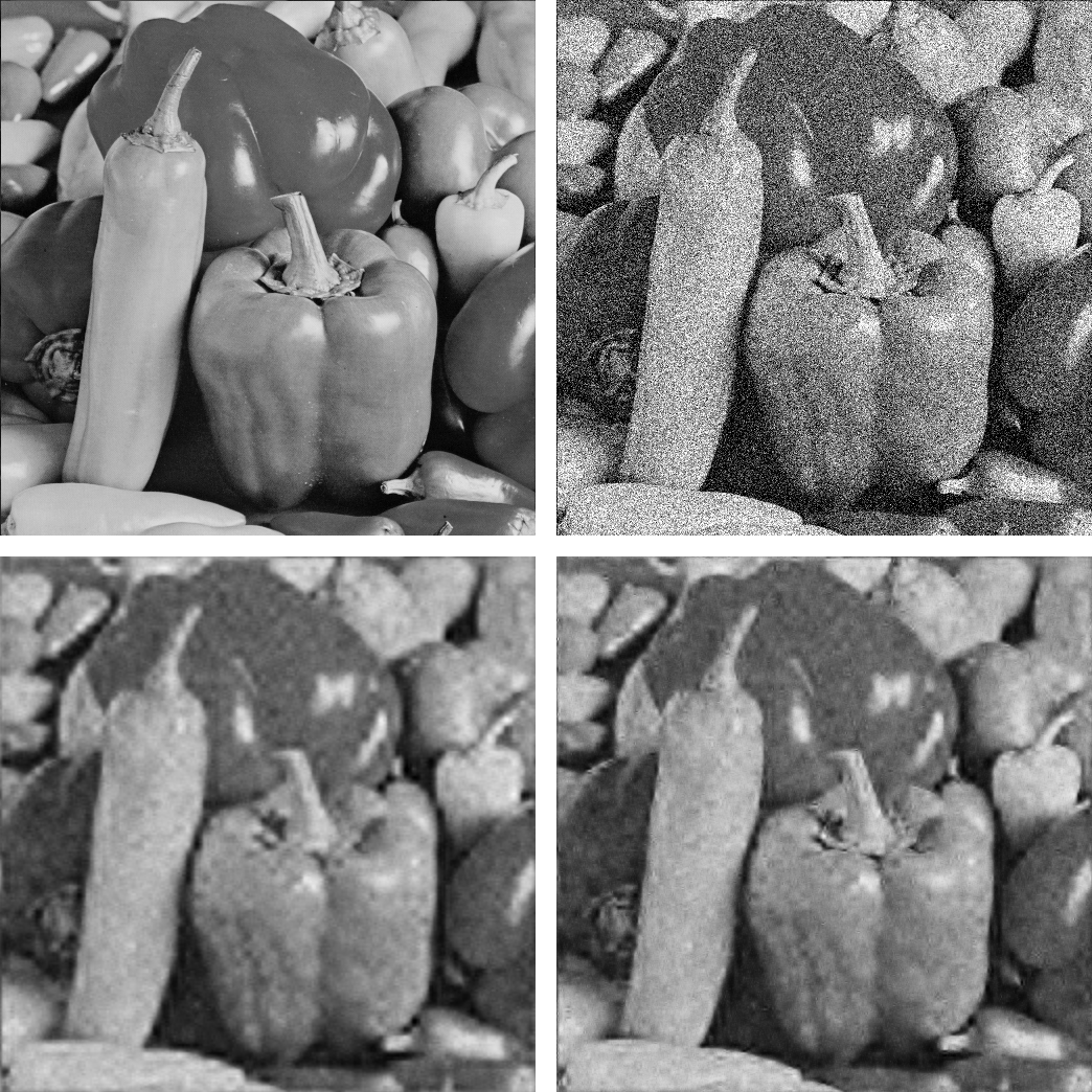
Figure 6: Denoising results for the peppers image from Table 3 when the standard deviation of the noise is 0.20. Top left panel: The original image. Top right panel: The noisy image (PSNR is 13.57). Bottom image: The noisy image cleaned using the GLG model and the composite EM algorithm (PSNR is 24.41).

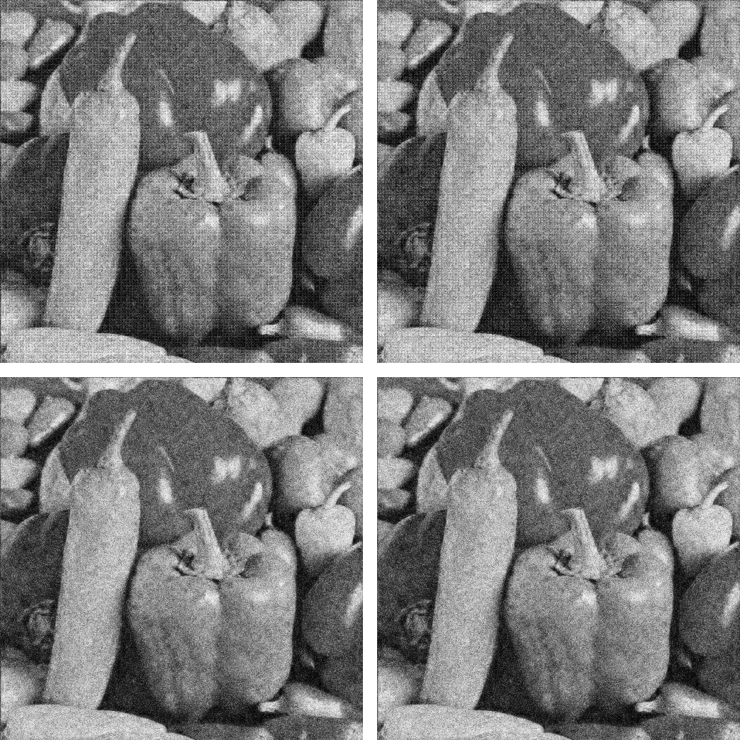
Figure 7: Denoising the ’peppers’ image using the posterior distribution (17) and INLA. The original and noisy images are seen in Figure 6. The top left, top right, and bottom left images are based on the 25%, 75%, and 50% quantiles of the posterior distribution, respectively (the PSNRs are 16.38, 16.41, and 19.18, respectively). The bottom right image is based on the mean of the posterior distribution (PSNR is 19.15). The posterior mean and median are almost identical.

6.2 Edge detection

Edge detection in an image is performed by labelling each pixel as being either an edge or a non-edge. Using the wavelet transform for this task has the advantage that wavelet coefficients are large near edges and small in the homogeneous parts of an image; the difficulty lies in quantifying ‘large’ and ‘small’. Another advantage is that a multiresolution analysis allows us to search for edges that are present at only selected scales of the image, that is, edges that are neither too coarse nor too fine.

This section discusses how to label the wavelet coefficient $w_{i}^{(t)}(\ell)$ by an indicator variable $f_{i}^{(t)}(\ell)$ so that $f_{i}^{(t)}(\ell)=1$ indicates that $w_{i}^{(t)}(\ell)$ is ‘large’ and $f_{i}^{(t)}(\ell)=0$ indicates that $w_{i}(\ell)^{(t)}$ is ‘small’. Our procedure is inspired by that of [12] which uses the 2-state Gaussian Finite Mixture (GFM) model of [1]. Below we recap this labelling algorithm, modify it to the case of our GLG model, and discuss how to transfer the labels $f_{i}^{(t)}(\ell)$ to the pixels. Finally, we show examples of both the original procedure using the GFM model and our modified procedure using the GLG model.

For our brief description of the edge detection algorithm in [12] it is sufficient to consider the 2-state GFM model based on a conditional independence structure as in (2), but where the hidden states take only binary values, indicating whether the associated wavelet coefficient is large or not. The labelling in [12] consists of three steps. First, using the EM algorithm an estimate ${\widehat{\bm{\theta}}}$ of the parameter vector $\bm{\theta}$ of a 2-state GFM model is obtained from the data ${\bar{\mathbf{w}}}$. Second, using an empirical Bayesian approach, the maximum a posteriori (MAP) estimate of the hidden states

$$\widehat{\mathbf{s}^{(t)}}=\operatorname*{argmax}_{\mathbf{s}^{(t)}}p(\mathbf{s}^{(t)}|\mathbf{w}^{(t)},{\widehat{\bm{\theta}}})=\operatorname*{argmax}_{\mathbf{s}^{(t)}}p(\mathbf{s}^{(t)},\mathbf{w}^{(t)}|{\widehat{\bm{\theta}}}),\quad t=1,\ldots,k,$$ (18)

is computed. Finally, they define $f_{i}^{(t)}(\ell)={\widehat{s^{(t)}_{i}(\ell)}}$.

The idea of labelling wavelet coefficients with the GLG model is overall the same as presented above for the GFM model, with the differences arising from the continuous nature of the hidden states and from different algorithms being applied for parameter estimation and state estimation. First, an estimate ${\widehat{\bm{\theta}}}$ of the parameter vector of the GLG model is obtained. Second, in analogy with (18) we compute the MAP estimate ${\widehat{\mathbf{s}^{(t)}}}$ by noting that

$$p(\mathbf{s}^{(t)},\mathbf{w}^{(t)}|{\widehat{\bm{\theta}}})=p(\mathbf{s}^{(t)}|{\widehat{\bm{\theta}}})\prod_{i=1}^{n}\prod_{\ell=1}^{d}p\bigl{(}w_{i}^{(t)}(\ell)|s^{(t)}_{i}(\ell)\bigr{)}$$ (19)

where $p(\mathbf{s}^{(t)}|{\widehat{\bm{\theta}}})$ is a multidimensional Gaussian density function those estimated mean vector and precision matrix are denoted ${\widehat{\bm{\mu}}}$ and $\widehat{\Delta}$, respectively. The log of (19) and its gradient vector and Hessian matrix with respect to $\mathbf{s}^{(t)}$ are

$$\log p(\mathbf{s}^{(t)},\mathbf{w}^{(t)}|{\widehat{\bm{\theta}}})\equiv-\frac{1}{2}\Bigl{\{}(\mathbf{s}^{(t)}-{\widehat{\bm{\mu}}})^{\top}\widehat{\Delta}(\mathbf{s}^{(t)}-{\widehat{\bm{\mu}}})+\sum_{i=1}^{n}\sum_{\ell=1}^{d}\bigl{(}w^{(t)}_{i}(\ell)^{2}\exp(-s^{(t)}_{i}(\ell))+s^{(t)}_{i}(\ell)\bigr{)}\Bigr{\}},$$

$$\nabla\log p(\mathbf{s}^{(t)},\mathbf{w}^{(t)}|{\widehat{\bm{\theta}}})=-\widehat{\Delta}(\mathbf{s}^{(t)}-{\widehat{\bm{\mu}}})+\frac{1}{2}\bigl{[}w^{(t)}_{i}(\ell)^{2}\exp(-s^{(t)}_{i}(\ell))-1\bigr{]}_{\ell=1,\ldots,d,\,i=1,\ldots,n},$$

$$H\bigl{(}\log p(\mathbf{s}^{(t)},\mathbf{w}^{(t)})\bigr{|}{\widehat{\bm{\theta}}})=-\widehat{\Delta}-\frac{1}{2}\operatorname{\text{diag}}\bigl{(}w^{(t)}_{i}(\ell)^{2}\exp(-s^{(t)}_{i}(\ell)),\,\ell=1,\ldots,d,\,i=1,\ldots,n\bigr{)},$$

where $\equiv$ means that an additive term which is not depending on $\mathbf{s}^{(t)}$ has been omitted in the right hand side expression. The Hessian matrix is strictly negative definite for all $(\mathbf{s}^{(t)},\mathbf{w}^{(t)})$ with $\mathbf{w}^{(t)}\neq\bm{0}$, and hence $\widehat{\mathbf{s}^{(t)}}$ can be found by solving $\nabla\log p(\mathbf{s}^{(t)},\mathbf{w}^{(t)}|{\widehat{\bm{\theta}}})=0$ using standard numerical tools. Finally, observe that if the estimate ${\widehat{s^{(t)}_{i}(\ell)}}$ is deemed to be large in the estimated distribution $N({\widehat{\mu_{\rho(i)}}},{\widehat{\sigma^{2}_{\rho(i)}}})$ for $s^{(t)}_{i}(\ell)$, then we expect $w^{(t)}_{i}(\ell)$ to be ‘large’. Therefore, denoting $z_{p}$ the $p$-quantile in $N({\widehat{\mu_{\rho(i)}}},{\widehat{\sigma_{\rho(i)}^{2}}})$, with e.g. $p=0.9$, we define $f^{(t)}_{i}(\ell)=1$ if ${\widehat{s^{(t)}_{i}(\ell)}}\geq z_{p}$ and $f^{(t)}_{i}(\ell)=0$ otherwise.

It remains to clarify how to transfer $f_{i}^{(t)}(\ell)$ (defined by one of the two methods above) to the pixel domain (this issue is not discussed in [12]). That is, we want specify a binary iamge with pixel values $e_{j}$ indicating whether pixel $j$ is part of an edge or not. Applying the inverse wavelet transform (with low-pass coefficients that are zero) to the label trees $\mathbf{f}^{(t)}$, $t=1,\ldots,k$, give an image with pixel values $\tilde{e}_{j}$, say. Since the wavelet transform does not necessarily map binary values to binary values, we define

$$e_{j}=\begin{dcases}1&\text{if }\widetilde{e}_{j}\neq 0,\\ 0&\text{otherwise}.\end{dcases}$$

The $e_{j}$’s are sensitive to the choice of wavelet transform, and using e.g. the Haar wavelet results in thin edges.

As mentioned, the multiresolution analysis of the wavelet transform allows us to consider edges with properties that are present at only specific scales. To exclude edges at a given level $r$, direction $\ell$ and tree $t$ in the wavelet transform, we simply modify $f^{(t)}_{i}(\ell)$ by setting $f^{(t)}_{i}(\ell)=0$ whenever $r(i)=r$.

Figure 8 compares the results of the two edge detection algorithms, when we only used the finest scale in the wavelet transform, and where in the case of our method the directional independence GLG model and the composite EM algorithm were used. Our method classified fewer pixels as edges, and comparing with Figure 4 it appears that the GFM-based procedure includes many superfluous pixels.

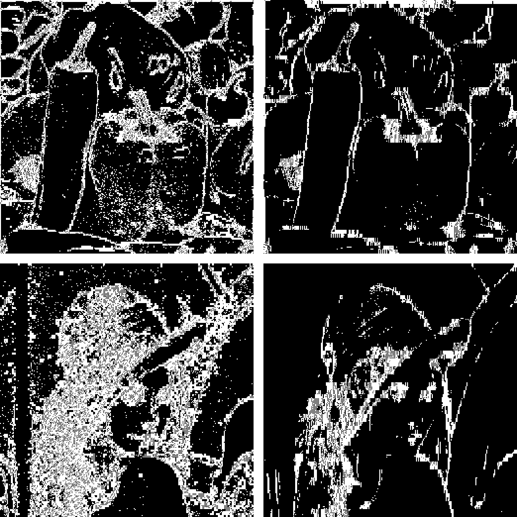
Figure 8: Examples of edge detection of the ’Lena’ and ’peppers’ images using the method from [12] (left column) and our variant that uses the GLG model (right column), when using a 3 level Haar wavelet transform and the $90\%$-quantile for thresholding with the GLG model, and considering only the finest level of the wavelet transform.

Appendix A Moments and estimating equations

This appendix specifies the moment estimates briefly discussed in Section 3.1.

Let $i$ be a node on level $r=r(i)$. Using (1) and (6), conditioning on the hidden states and exploiting the conditional independence structure, we obtain

$$\eta_{r,\ell}^{(2)} :=\operatorname{E}\bigl{[}w_{i}(\ell)^{2}\bigr{]}=\exp\Bigl{(}\mu_{r,\ell}+\sigma_{r,\ell,\ell}/2\Bigr{)},$$ (20)

$$\eta_{r,\ell}^{(4)} :=\operatorname{E}\bigl{[}w_{i}(\ell)^{4}\bigr{]}=3\exp\Bigl{(}2\mu_{r,\ell}+2\sigma_{r,\ell,\ell}\Bigr{)},$$ (21)

for $1\leq\ell\leq d$,

$$\eta_{r,\ell,\ell^{\prime}}^{(2,2)} :=\operatorname{E}\bigl{[}w_{i}(\ell)^{2}w_{i}(\ell^{\prime})^{2}\bigr{]}$$

$$=\exp\Bigl{(}\mu_{r,\ell}+\mu_{r,\ell^{\prime}}+\sigma_{r,\ell,\ell}/2+\sigma_{r,\ell^{\prime},\ell^{\prime}}/2+\sigma_{r,\ell,\ell^{\prime}}\Bigr{)},$$ (22)

for $1\leq\ell<\ell^{\prime}\leq d$, and if $r<L$ and $j\in c(i)$, then

$$\xi_{r,\ell,\ell^{\prime}}^{(2,2)} :=\operatorname{E}\bigl{[}w_{i}(\ell)^{2}w_{j}(\ell^{\prime})^{2}\bigr{]}$$

$$=\exp\bigl{(}\mu_{r,\ell}+\mu_{r+1,\ell^{\prime}}+\sigma_{r,\ell,\ell}/2+\sigma_{r+1,\ell^{\prime},\ell^{\prime}}/2+\sum_{k=1}^{d}\beta_{r,\ell,k}\sigma_{r,k,\ell^{\prime}}\bigr{)},$$ (23)

for $1\leq\ell,\ell^{\prime}\leq d$. Let $n_{r}$ denote the number of nodes on level $r$. Using the unbiased estimates of $\eta_{r,\ell}^{(2)}$, $\eta_{r,\ell}^{(4)}$, $\eta_{r,\ell,\ell^{\prime}}^{(2,2)}$ given by

$$\eta_{r,\ell}^{(a)} =\frac{1}{kn_{r}}\sum_{t=1}^{k}\sum_{i:r(i)=r}\sum_{j\in c(i)}\bigl{(}w_{j}(\ell)^{(t)}\bigr{)}^{a},\quad a=2,4,$$

$$\eta_{r,\ell,\ell^{\prime}}^{(2,2)} =\frac{1}{kn_{r}}\sum_{t=1}^{k}\sum_{i:r(i)=r}\sum_{j\in c(i)}\bigl{(}w_{j}(\ell)^{(t)}\bigr{)}^{2}\bigl{(}w_{j}(\ell^{\prime})^{(t)}\bigr{)}^{2},$$

$$\xi_{r,\ell,\ell^{\prime}}^{(2,2)} =\frac{1}{kn_{r}}\sum_{t=1}^{k}\sum_{i:r(i)=r}\sum_{j\in c(i)}\bigl{(}w_{i}(\ell)^{(t)}\bigr{)}^{2}\bigl{(}w_{j}(\ell^{\prime})^{(t)}\bigr{)}^{2},$$

(20)- (22) can be solved to obtain estimates ${\widehat{\bm{\mu}_{r}}}$ and ${\widehat{\bm{\Sigma}_{r}}}$. Combining the estimates $\widehat{\bm{\mu}_{r}}$, $\widehat{\bm{\Sigma}_{r}}$, $\widehat{\xi}_{r,\ell,\ell^{\prime}}^{(2,2)}$ with (23) we obtain an estimate ${\widehat{\bm{B}_{r}}}$. Finally, combining these estiamtes with (7) we obtain estimates ${\widehat{\bm{\alpha}_{r}}}$ and ${\widehat{\bm{K}_{r}}}$.

The estimating equations (20)- (23) do not guarantee that the estimated covariance matrices are strictly positive definite. Therefore the estimates of $\bm{\Sigma}_{r}$ and $\bm{K}_{r}$ are replaced by the positive definite matrices that are closest in the Frobenius norm. This choice of norm is due to the simple analytical solution of the positive definite approximant [5].

Appendix B EM algorithm for marginal likelihoods

The EM algorithm [2, 3] is an iterative estimation procedure which applies for steps 1 and 2 in Section 3.2.2 as described below.

We start by noticing that the conditional density of $\bm{s}_{1}$ given $\bm{w}_{1}$ is

$$p(\bm{s}_{1}|\bm{w}_{1},\bm{\mu}_{1},\bm{\Sigma}_{1})=\frac{p(\bm{s}_{1},\bm{w}_{1}\,|\,\bm{\mu}_{1},\bm{\Sigma}_{1})}{q(\bm{w}_{1}\,|\,\bm{\mu}_{1},\bm{\Sigma}_{1})}$$

$$\propto\exp\biggl{(}-\frac{1}{2}\biggl{\{}\biggl{[}\sum_{\ell=1}^{d}\frac{w_{1}(\ell)^{2}}{\exp(s_{1}(\ell))}+s_{1}(\ell)\biggr{]}+(\bm{s}_{1}-\bm{\mu}_{1})^{\top}\bm{\Sigma}_{1}^{-1}(\bm{s}_{1}-\bm{\mu}_{1})\biggr{\}}\biggr{)}$$ (24)

where in the expression on the right hand side we have omitted a factor which does not depend on the argument $\bm{s}_{1}$ of the conditional density. Note also that for $r(i)=r<L$, the conditional density of $\bm{s}_{i,c(i)}$ given $\bm{w}_{i,c(i)}$ is

$$p(\bm{s}_{i,c(i)}\,|\,\bm{w}_{i,c(i)},\bm{\mu}_{r-1},\bm{\Sigma}_{r-1},\bm{\alpha}_{r},\bm{B}_{r},\bm{K}_{r})=\frac{p(\bm{s}_{i,c(i)},\bm{w}_{i,c(i)}\,|\,\bm{\mu}_{r-1},\bm{\Sigma}_{r-1},\bm{\alpha}_{r},\bm{B}_{r},\bm{K}_{r})}{q(\bm{w}_{i,c(i)}\,|\,\bm{\mu}_{r-1},\bm{\Sigma}_{r-1},\bm{\alpha}_{r},\bm{B}_{r},\bm{K}_{r})}$$

$$\propto\exp\biggl{(}-\frac{1}{2}\biggl{\{}\biggl{[}\sum_{\ell=1}^{d}\frac{w_{i}(\ell)^{2}}{\exp(s_{i}(\ell))}+s_{i}(\ell)\biggr{]}+(\bm{s}_{i}-\bm{\mu}_{r-1})^{\top}\bm{\Sigma}_{r-1}^{-1}(\bm{s}_{i}-\bm{\mu}_{r-1})$$

$$+\sum_{j\in c(i)}\biggl{[}\sum_{\ell=1}^{d}\frac{w_{j}(\ell)^{2}}{\exp(s_{j}(\ell))}+s_{j}(\ell)\biggr{]}+(\bm{s}_{j}-\bm{\alpha}_{r}-\bm{B}_{r}\bm{s}_{i})^{\top}\bm{K}_{r}^{-1}(\bm{s}_{j}-\bm{\alpha}_{r}-\bm{B}_{r}\bm{s}_{i})\biggr{\}}\biggr{)}$$ (25)

In step 1, suppose $(\bm{\mu}_{1}^{\prime},\bm{\Sigma}_{1}^{\prime})$ is a current estimate. We consider the conditional expectation with respect to (24) when $(\bm{\mu}_{1},\bm{\Sigma}_{1})$ is replaced by $(\bm{\mu}_{1}^{\prime},\bm{\Sigma}_{1}^{\prime})$. Then the next estimate for $(\bm{\mu}_{1},\bm{\Sigma}_{1})$ is the maximum point for the conditional expectation of the log-likelihood which is based on both $\overline{\bm{w}}_{1}$ and $\overline{\bm{s}}_{1}$; this log-likelihood is given by

$$\sum_{t=1}^{k}\log p(\bm{w}_{1}^{(t)},\bm{s}_{1}^{(t)}\,\big{|}\,\bm{\mu}_{1},\bm{\Sigma}_{1})\equiv-\frac{1}{2}\sum_{t=1}^{k}\Bigl{[}\log\det(\bm{\Sigma}_{1})+(\bm{s}_{1}-\bm{\mu}_{1})^{\top}\bm{\Sigma}_{1}^{-1}(\bm{s}_{1}-\bm{\mu}_{1})\Bigr{]}$$

where $\equiv$ means that an additive term which is not depending on $(\bm{\mu}_{1},\bm{\Sigma}_{1})$ has been omitted in the right hand side expression, cf. (8). It is well-known from the theory of estimation in the multivariate Gaussian distribution that the maximum point is given by

$$\widehat{\bm{\mu}}_{1}=\frac{1}{k}\sum_{t=1}^{k}\operatorname{E}\Bigl{[}\bm{s}_{1}^{(t)}\,|\,\bm{w}_{1}^{(t)},\bm{\mu}_{1}^{\prime},\bm{\Sigma}_{1}^{\prime}\Bigr{]},$$ (26)

$$\widehat{\bm{\Sigma}}_{1}=\biggl{\{}\frac{1}{k}\sum_{t=1}^{k}\operatorname{E}\Bigl{[}\bm{s}_{1}^{(t)}\bigl{(}\bm{s}_{1}^{(t)}\bigr{)}^{\top}\,|\,\bm{w}_{1}^{(t)},\bm{\mu}_{1}^{\prime},\bm{\Sigma}_{1}^{\prime}\Bigr{]}\biggr{\}}-\widehat{\bm{\mu}}_{1}\widehat{\bm{\mu}}_{1}^{\top},$$ (27)

where the conditional expectations are calculated using (24). As mentioned in Section 3.2.1, the integrals are calculated using the Gauss-Hermite quadrature rule. The iteration is repeated with $(\bm{\mu}_{1}^{\prime},\bm{\Sigma}_{1}^{\prime})=(\widehat{\bm{\mu}}_{1},\widehat{\bm{\Sigma}}_{1})$ until convergence is effectively obtained, whereby a final estimate $(\widehat{\bm{\mu}}_{1},\widehat{\bm{\Sigma}}_{1})$ is returned.

In step 2, suppose $(\bm{\alpha}_{r}^{\prime},\bm{B}_{r}^{\prime},\bm{K}_{r}^{\prime})$ is a current estimate, which we use together with the estimate $(\widehat{\bm{\mu}}_{r},\widehat{\bm{\Sigma}}_{r})$ to obtain the next estimate for $(\bm{\alpha}_{r},\bm{B}_{r},\bm{K}_{r})$: Replacing $(\bm{\mu}_{r},\bm{\Sigma}_{r},\bm{\alpha}_{r},\bm{B}_{r},\bm{K}_{r})$ by $(\widehat{\bm{\mu}}_{r},\widehat{\bm{\Sigma}}_{r},\bm{\alpha}_{r}^{\prime},\bm{B}_{r}^{\prime},\bm{K}_{r}^{\prime})$, this estimate is the maximum point for the conditional expectation with respect to (25) of each term in the sum

$$\sum_{t=1}^{k}\sum_{i:r(i)=r}\log p(\bm{w}_{i,c(i)}^{(t)},\bm{s}_{i,c(i)}^{(t)}\,\big{|}\,\widehat{\bm{\mu}}_{r},\widehat{\bm{\Sigma}}_{r},\bm{\alpha}_{r},\bm{B}_{r},\bm{K}_{r})$$

$$\equiv-\frac{1}{2}\sum_{t=1}^{k}\sum_{i:r(i)=r}\sum_{j\in c(i)}\Bigl{[}\log\det(\bm{K}_{r})+(\bm{s}_{j}-\bm{\alpha}_{r}-\bm{B}_{r}\bm{s}_{i})^{\top}\bm{K}_{r}^{-1}(\bm{s}_{j}-\bm{\alpha}_{r}-\bm{B}_{r}\bm{s}_{i})\Bigr{]},$$

where additive terms which do not depend on $(\bm{\alpha}_{r},\bm{B}_{r},\bm{K}_{r})$ have been omitted, cf. (11). For $1\leq r<L$, let $n_{r}=\#\{i\,:\,r(i)=r\}$ and

$$\overline{\bm{s}}(r)=\frac{1}{kn_{r}}\sum_{t=1}^{k}\sum_{i:r(i)=r}\operatorname{E}\Bigl{[}\bm{s}_{k}^{(t)}\,\Big{|}\,\bm{w}_{i,c(i)}^{(t)},\widehat{\bm{\mu}}_{r},\widehat{\bm{\Sigma}}_{r},\bm{\alpha}_{r}^{\prime},\bm{B}_{r}^{\prime},\bm{K}_{r}^{\prime}\Bigr{]}.$$

Then, by the theory of multiple linear regression, the maximum point is given by

$$\widehat{\bm{B}}_{r} =\biggl{\{}\sum_{t=1}^{k}\sum_{i:r(i)=r}|c(i)|\operatorname{E}\Bigl{[}\bm{s}_{i}^{(t)}\bigl{(}\bm{s}_{i}^{(t)}\bigr{)}^{\top}-\overline{\bm{s}}(r)\overline{\bm{s}}(r)^{\top}\,\Big{|}\,\bm{w}_{i,c(i)}^{(t)},\widehat{\bm{\mu}}_{r},\widehat{\bm{\Sigma}}_{r},\bm{\alpha}_{r}^{\prime},\bm{B}_{r}^{\prime},\bm{K}_{r}^{\prime}\Bigr{]}\biggr{\}}^{-1}$$

$$\quad\sum_{t=1}^{k}\sum_{i:r(i)=r}\sum_{j\in c(i)}\operatorname{E}\Bigl{[}\bm{s}_{j}^{(t)}\bigl{(}\bm{s}_{i}^{(t)}-\overline{\bm{s}}(r)\bigr{)}^{\top}\,\Big{|}\,\bm{w}_{i,c(i)}^{(t)},\widehat{\bm{\mu}}_{r},\widehat{\bm{\Sigma}}_{r},\bm{\alpha}_{r}^{\prime},\bm{B}_{r}^{\prime},\bm{K}_{r}^{\prime}\Bigr{]}$$ (28)

$$\widehat{\bm{\alpha}}_{r} =\overline{\bm{s}}(r+1)-\widehat{\bm{B}}_{r}\overline{\bm{s}}(r),$$ (29)

$$\widehat{\bm{K}}_{r} =\frac{1}{kn_{r}}\sum_{t=1}^{k}\sum_{i:r(i)=r}\frac{1}{|c(i)|}\sum_{j\in c(i)}$$

$$\quad\operatorname{E}\Bigl{[}(\bm{s}_{j}^{(t)}-\widehat{\bm{B}}_{r}\bm{s}_{i}^{(t)})(\bm{s}_{j}^{(t)}-\widehat{\bm{B}}_{r}\bm{s}_{i}^{(t)})^{\top}\,\Big{|}\,\bm{w}_{i,c(i)}^{(t)},\widehat{\bm{\mu}}_{r},\widehat{\bm{\Sigma}}_{r},\bm{\alpha}_{r}^{\prime},\bm{B}_{r}^{\prime},\bm{K}_{r}^{\prime}\Bigr{]}-\widehat{\bm{\alpha}}_{r}\widehat{\bm{\alpha}}_{r}^{\top}.$$ (30)

The iteration is repeated with $(\bm{\alpha}_{r}^{\prime},\bm{B}_{r}^{\prime},\bm{K}_{r}^{\prime})=(\widehat{\bm{\alpha}}_{r},\widehat{\bm{B}}_{r},\widehat{\bm{K}}_{r})$ until convergence is effectively obtained, whereby a final estimate $(\widehat{\bm{\alpha}}_{r},\widehat{\bm{B}}_{r},\widehat{\bm{K}}_{r})$ is returned.

Appendix C Conditional expectation of noisy observations

Let the situation be as in Section 6.1 and consider the GLG model. The joint density of $(s,v)$ is found just as in the noise-free case in (8),

$$p(s,v|\mu,\sigma^{2})=p(v|s)p(s|\mu,\sigma^{2})=\frac{\exp\Bigl{(}-\frac{1}{2}\Bigl{[}\frac{v^{2}}{\exp(s)+\sigma_{\varepsilon}^{2}}+\frac{(s-\mu)^{2}}{\sigma^{2}}\Bigr{]}\Bigr{)}}{2\pi\sigma\sqrt{\exp(s)+\sigma_{\varepsilon}^{2}}}$$

and the marginal density of the wavelet with noise is

$$p(v|\mu,\sigma^{2})=\int_{-\infty}^{\infty}p(s,v|\mu,\sigma^{2})\,\mathrm{d}s.$$

We do not have a closed form expression for this integral, but due to the form of the integrant we approximate the integral with the Gauss-Hermite quadrature rule, see e.g. [8]. The conditional density of $s$ given $v$ is

$$p(s|v,\mu,\sigma^{2})=\frac{p(s,v|\mu,\sigma^{2})}{p(v|\mu,\sigma^{2})}=\frac{\exp\Bigl{(}-\frac{1}{2}\Bigl{[}\frac{v^{2}}{\exp(s)+\sigma_{\varepsilon}^{2}}+\frac{(s-\mu)^{2}}{\sigma^{2}}\Bigr{]}\Bigr{)}}{c(v|\mu,\sigma^{2})\sqrt{\exp(s)+\sigma_{\varepsilon}^{2}}}$$

where $c(v|\mu,\sigma^{2})=2\pi\sigma p(v|\mu,\sigma^{2})$. Furthermore, from well-known results about the bivariate normal distribution we obtain

$$\operatorname{E}[w|s,v,\bm{\theta}]=\frac{\operatorname{Cov}[w,v|s,\bm{\theta}]}{\operatorname{Var}[v|s,\bm{\theta}]}v=\frac{\operatorname{Var}[w|s]}{\operatorname{Var}[v|s]}v=\frac{\exp(s)}{\exp(s)+\sigma_{\varepsilon}^{2}}v.$$

Hence

$$\operatorname{E}[w|v,\bm{\theta}]=\operatorname{E}\bigl{[}\operatorname{E}[w|s,v,\bm{\theta}]\big{|}v,\bm{\theta}\bigr{]}=v\,\operatorname{E}\biggl{[}\frac{\exp(s)}{\exp(s)+\sigma_{\varepsilon}^{2}}\bigg{|}v,\bm{\theta}\biggr{]}$$ (31)

whereby we obtain (16).

References

• [1] Matthew S. Crouse, Robert D. Nowak, and Richard G. Baraniuk. Wavelet-based statistical signal processing using hidden Markov models. IEEE Transactions on Signal Processing, 46(4):886–902, 4 1998.
• [2] A. P. Dempster, N. M. Laird, and D. B. Rubin. Maximum likelihood from incomplete data via the EM algorithm. Journal of the Royal Statistical Society: Series B (Statistical Methodology), 39(1):1–38, 1977.
• [3] Xin Gao and Peter X.-K. Song. Composite likelihood EM algorithm with applications to multivariate hidden Markov model. Statistica Sinica, 21(1):165–185, 2011.
• [4] Florian Heiss and Viktor Winschel. Likelihood approximation by numerical integration on sparse grids. Journal of Econometrics, 144(1):62–80, 5 2008.
• [5] Nicholas J. Higham. Computing a nearest symmetric positive semidefinite matrix. Linear Algebra and its Applications, 103:103–118, 1988.
• [6] Steffen L. Lauritzen. Graphical Models. Clarendon Press, Oxford, 1996.
• [7] Thiago G. Martins, Daniel Simpson, Finn Lindgren, and Håvard Rue. Bayesian computing with INLA: new features. Computational Statistics and Data Analysis, 67:68–83, 11 2013.
• [8] William H. Press, Saul A. Teukolsky, William T. Vetterling, and Brian P. Flannery. Numerical Recipes in C++. Cambridge University Press, Cambridge, 2 edition, 2002.
• [9] R Core Team. R: A Language and Environment for Statistical Computing. R Foundation for Statistical Computing, Vienna, Austria, 2016.
• [10] Håvard Rue and Sara Martino. Approximate Bayesian inference for hierarchical Gaussian Markov random field models. Journal of Statistical Planning and Inference, 137(11):3177–3192, 2007.
• [11] Håvard Rue, Sara Martino, and Nicolas Chopin. Approximate Bayesian inference for latent Gaussian models by using integrated nested Laplace approximations. Journal of the Royal Statistical Society: Series B (Statistical Methodlogy), 71(2):319–392, 2009.
• [12] Junxi Sun, Dongbing Gu, Yazhu Chen, and Su Zhang. A multiscale edge detection algorithm based on wavelet domain vector hidden Markov tree model. Pattern Recognition, 37(7):1315–1324, 2004.
• [13] Martin J. Wainwright, Eero P. Simoncelli, and Alan S. Willsky. Random cascades on wavelet trees and their use in analyzing and modeling natural images. Applied and Computational Harmonic Analysis, 11(1):89–123, 2001.