A Polynomial Scheme of Asymptotic Expansion
for Backward SDEs and Option pricing

Abstract

A new asymptotic expansion scheme for backward SDEs (BSDEs) is proposed. The perturbation parameter “$\epsilon$” is introduced just to scale the forward stochastic variables within a BSDE. In contrast to the standard small-diffusion asymptotic expansion method, the dynamics of variables given by the forward SDEs is treated exactly. Although it requires a special form of the quadratic covariation terms of the continuous part, it allows rather generic drift as well as jump components to exist. The resultant approximation is given by a polynomial function in terms of the unperturbed forward variables whose coefficients are uniquely specified by the solution of the recursive system of linear ODEs. Applications to a jump-extended Heston and $\lambda$-SABR models for European contingent claims, as well as the utility-optimization problem in the presence of a terminal liability are discussed.

Keywords : Stochastic Control, Asymptotic Expansion, BSDE, random measure, Heston, SABR, Utility optimization

1 Introduction

The backward stochastic differential equation (BSDE) was introduced by Bismut (1973) [2] under a linear setup and was later extended by Pardoux & Peng (1990) [29] to general non-linear situations. Although the research activity had been contained in a relatively small mathematical community, it has been rapidly gaining traction with financial researchers and practitioners, in particular, since the last financial crisis. This is because that one almost inevitably encounters BSDEs when he/she tries to handle various non-linear effects arising from credit risk, collateralization, funding and regulatory costs, and various other sources of incompleteness arising from the new market realities. See, for example, Duffie & Huang (1996) [14], Fujii & Takahashi (2013) [16], Crépey (2013) [9] and a summary of recent practical topics in the financial industry [3, 5]. Various interesting financial applications, such as for insurance, utility indifference pricing and optimal contract theory can be found in books [12, 7, 11, 10]. One can consult with [15, 25] as a text for general mathematical treatments of BSDEs.

There now exists vast literature on their numerical treatments, ranging from the famous four-step scheme proposed by Ma et al. (1994) [26], its discretized implementation by Douglas et al. (1996) [13], various Monte-Carlo techniques making use of the least-square regression method (See, for example, Bouchard & Touzi (2004) [6], Bender & Denk (2007) [1], Gobet et al. (2005) [21] and Gobet & Lemor (2010) [22]), a branching diffusion method by Henry-Labordere (2012) [23], and a particle method by Fujii & Takahashi (2012a) [17]. Unfortunately though, many of them require a good amount of experience and deep expertise to achieve stable results, such as an appropriate choice of basis functions, the order of regressions, and of course, a good programming technique.

It is obvious that a simple analytical approximation method is deeply wanted. In Fujii & Takahashi (2012b) [18], we have developed a driver perturbation method combined with a standard asymptotic expansion technique for the forward SDEs. Its error estimate was recently provided by Takahashi & Yamada (2013) [33]. It is systematic and straightforward, but one still needs to endure long tough calculations especially for higher order corrections, which is stemming from the needs of evaluation of conditional expectations at each order of expansion. An interesting exceptional case arises if a so-called quadratic-growth BSDE (qgBSDE) is associated with linear Gaussian forward SDEs, and at the same time, if its terminal value is given by, at most, quadratic form of the Gaussian variables. In this case, the value function is given by a quadratic function of the Gaussian variables whose coefficients are completely determined by the ordinary differential equations (ODEs) involving ones with Riccati form. See, for example, Schroder & Skiadas (1999) [31] as an early research. Recently, this property was applied to the mean-variance (quadratic) hedging problem by Fujii & Takahashi (2013, 2014) [19, 20], making use of the beautiful BSDE expression derived by Mania & Tevzadze (2003) [27]. Notice that the Riccati equation may possibly diverge in a finite time-interval in a general setup. In such a case, one needs to shorten the maturity of the corresponding problem.

In this paper, we propose a new scheme which approximates a solution of a BSDE by a polynomial function of the underlying variables. In a Markovian setup, it is well-known that the solution of a BSDE is given by a Markovian function of the underlying variables [26]. Therefore, it is intuitively clear that the solution should be well approximated by a polynomial function for short maturities within which the size of the underlying variables (after appropriate rescaling and shift of their means) remains relatively small. Despite the apparent similarity to the usual asymptotic expansion, the new scheme yields a recursive system of linear ODEs which can be obtained by simply matching the coefficients of the assumed polynomial solution to those of the BSDE’s driver. Although we have to assume that the forward processes have a special form of quadratic covariation of the continuous part, they can have rather general drifts and random jump components. In that sense, the method can be interpreted as a generalizations of exact but exceptional quadratic-solution example to an approximate polynomial-solution technique with wider applications.

The organization of the paper is as follows: In Section 2, the main idea of the polynomial expansion scheme is explained. In order to show its usefulness and accuracy, we apply the method to several well-known problems in the remaining part of the paper. In Section 3 and 4, the proposed scheme is applied to European contingent claims using a jump-extended Heston model and the $\lambda$-SABR model. We provide the closed expression for the recursive system of linear ODEs which specifies the approximate solution at an arbitrary order. In Section 5, the optimization problem for the exponential utility in the presence of a terminal liability is analyzed. The closed-form system of the linear ODEs is derived for this setup, too. Each model is associated with several illustrative numerical examples. Finally in Appendix, some details omitted in the main text are provided.

2 Polynomial Expansion Scheme

2.1 Problem Setup

Let us consider the following system of forward and backward SDEs in a probability space $(\Omega,{\cal F},\mathbb{P})$:

$$V_{t} = H(X_{T})-\int_{t}^{T}\bar{f}\Bigl{(}s,X_{s},V_{s},\bar{Z}_{s},\int_{K}U(s,z)Q(s,dz)\Bigr{)}ds$$ (2.1)

$$-\int_{t}^{T}\bar{Z}_{s}dW_{s}-\int_{t}^{T}\int_{K}U(s,z)\widetilde{{\cal N}}(ds,dz)$$

$$X_{t} = x+\int_{0}^{t}b(s,X_{s})ds+\int_{0}^{t}\sigma(s,X_{s})dW_{s}+\int_{0}^{t}\int_{K}z{\cal N}(ds,dz)$$ (2.2)

where $x\in\mathbb{R}$ is a constant, $W$ one-dimensional standard Brownian motion and ${\cal N}$ a random measure whose deterministic jump distribution is given by $Q(t,\cdot)$ with some (compact) space $K$ for its support. $\widetilde{{\cal N}}(dt,dz)$ is the corresponding $\mathbb{P}$-compensated random measure

$$\widetilde{{\cal N}}(dt,dz):={\cal N}(dt,dz)-\lambda(t,X_{t})Q(t,dz)dt$$ (2.3)

where $\lambda(t,X_{t})$ denotes the jump intensity. We assume that $H:\mathbb{R}\rightarrow\mathbb{R}$, $\bar{f}:[0,T]\times\mathbb{R}^{4}\rightarrow\mathbb{R}$, $b:[0,T]\times\mathbb{R}\rightarrow\mathbb{R}$ and $\lambda:[0,T]\times\mathbb{R}\rightarrow\mathbb{R}_{+}$ are all smooth functions. In addition, we assume that the quadratic covariation of $X$ from its continuous part is given by, at most, quadratic form of $X$ itself

$$d\langle X^{c}\rangle_{t}=\Bigl{(}\sigma_{2}(t)X_{t}^{2}+\sigma_{1}(t)X_{t}+\sigma_{0}(t)\Bigr{)}dt~{}$$ (2.4)

where the superscript “$c$” denotes the continuous part of $X$. Here, $(\sigma_{i}(t))_{i=1,2,3}$ is the set of deterministic functions in such a way that it guarantees the right-hand side of (2.4) is non-negative for every possible value taken by $X$. We assume that the forward-backward SDE system of (2.1) and (2.2) has a well-posed solution.

Since the stochasticity of $(V_{t})_{t\geq 0}$ is provided solely by $(X_{t})_{t\geq 0}$, we can rewrite the BSDE as

$$V_{t} = H(X_{T})-\int_{t}^{T}f\Bigl{(}s,X_{s},V_{s},Z_{s},\int_{K}U(s,z)Q(s,dz)\Bigr{)}ds$$ (2.5)

$$-\int_{t}^{T}Z_{s}dX_{s}^{c}-\int_{t}^{T}\int_{K}U(s,z){\cal N}(ds,dz)$$

with appropriate redefinition of $f(\cdot)$ and $Z$ . Here, $dX_{t}^{c}:=b(t,X_{t})dt+\sigma(t,X_{t})dW_{t}$ denotes the continuous part of the $X$’s change. Thus, in the following, we consider the equivalent system given by $(\ref{BSDE-X})$ and $(\ref{SDE-X})$.

2.2 Asymptotic Expansion

2.2.1 General Idea

In order to obtain a polynomial expansion, we introduce $\epsilon$ so that we can count the order of the underlying $X$. Let consider the following perturbed BSDE:

$$V_{t}^{\epsilon} = H(\epsilon X_{T})-\int_{t}^{T}f\Bigl{(}s,\epsilon X_{s},V^{\epsilon}_{s},Z^{\epsilon}_{s},\int_{K}U^{\epsilon}(s,z)Q(s,dz)\Bigr{)}ds$$ (2.6)

$$-\int_{t}^{T}Z^{\epsilon}_{s}dX_{s}^{c}-\int_{t}^{T}\int_{K}U^{\epsilon}(s,z){\cal N}(ds,dz)~{}.$$

Here, the superscripts $\epsilon$ in $V,Z,U$ emphasizes that these variables are now dependent on the parameter $\epsilon$. An important difference from the usual small diffusion asymptotic expansion method proposed by (Yoshida (1992a) [35], Takahashi (1999) [32], Kunitomo & Takahashi (2003) [24] for the pricing of contingent claims, Yoshida (1992b) [36] for statistical applications ) based on Watanabe (1987) [34] theory is that the underlying process $(X_{t})_{t\geq 0}$ itself is not perturbed and only its size is scaled by $\epsilon$ within the BSDE.

We assume that that the expansion

$$V_{t}^{\epsilon} = \sum_{n=0}^{\infty}\epsilon^{n}V^{[n]}_{t}$$ (2.7)

$$V_{t}^{[n]} = \sum_{m=0}^{n}\frac{X_{t}^{m}}{m!}v^{[n]}_{m}(t)$$ (2.8)

is well defined, where $(v^{[n]}_{m}(t),0\leq m\leq n)$ are all deterministic bounded functions in a given time interval $t\in[0,T]$. In particular, the Itô-formula should be applicable to (2.8) so that one obtains the well-defined forward SDE for $(V^{[n]}_{t})_{0\leq t\leq T}$. It leads to the corresponding expansions of the control variables

$$Z_{t}^{\epsilon}=\sum_{n=0}^{\infty}\epsilon^{n}Z_{t}^{[n]}$$ (2.9)

$$U^{\epsilon}(t,z)=\sum_{n=0}^{\infty}\epsilon^{n}U^{[n]}(t,z)$$ (2.10)

whose expressions can be easily derived once (2.8) is obtained.

If the maturity is short enough so that size of $X$ remains small, truncating the expansion in (2.7) at a certain order $n$ and putting $(\epsilon=1)$ are expected to give an approximation of the original problem. Note that, since $\epsilon$ is introduced as a combination $(\epsilon X)$, discussing the size of $\epsilon$ separately from $X$ is not useful. Let us denote the truncated $n$-th order approximation as (using the superscript $(n)$ instead of $[n]$)

$$V_{t}^{(n)}=\sum_{j=0}^{n}V_{t}^{[j]}$$ (2.11)

$$Z_{t}^{(n)}=\sum_{j=0}^{n}Z_{t}^{[j]},\quad U^{(n)}(t,z)=\sum_{j=0}^{n}U^{[j]}(t,z)~{}.$$ (2.12)

Note that all of them are given by the polynomial functions of $X$, at most, of the order of $n$.

One can check the accuracy of approximation by comparing

$$\widetilde{V}^{(n)}(T) = V_{0}^{(n)}+\int_{0}^{T}f\Bigl{(}s,X_{s},V_{s}^{(n)},Z_{s}^{(n)},\int_{K}U^{(n)}(s,z)Q(s,dz)\Bigr{)}ds$$ (2.13)

$$+\int_{0}^{T}Z_{s}^{(n)}dX_{s}^{c}+\int_{0}^{T}\int_{K}U^{(n)}(s,z){\cal N}(ds,dz)$$

and $H(X_{T})$ in a “path-wise” fashion. In numerical examples given in later sections, we shall observe that the polynomial approximation gives a good path-wise approximation, at least for the paths along which $(|X_{t}(\omega)|)_{t\geq 0}$ does not significantly grow to a big value. In practical applications, the capability of checking $(H(X_{T})-\widetilde{V}^{(n)}(T))$ directly should be a great help for setting aside an appropriate amount of risk-reserve for the hedging program to be implemented. By the very nature of polynomial approximation, one can imagine that a higher order expansion may yield an unstable result in a very volatile market, or for a problem with long maturity. The above comparison gives useful information for an appropriate order of expansion for a given situation.

As we shall see below, all the functions $(v^{[n]}_{m}(t))_{m,n}$ except $v^{[0]}_{0}(t)$ are specified by linear ODEs. In later sections which deal with specific models, we provide a closed form recursive system of linear ODEs which fixes the coefficients of the polynomials up to an arbitrary order. However, in this section, let us adopt a slightly tedious step-by-step explanation, which we hope to give a clearer image to the readers.

2.2.2 Zero-th order

It is obvious that

$$V^{[0]}_{t}=H(0)-\int_{t}^{T}f(s)ds$$ (2.14)

where $f(s):=f(s,0,V_{s}^{[0]},0,0)$. Hence, the coefficient should be determined by

$$\dot{v}^{[0]}_{0}(t)=f(t,0,v_{0}^{[0]}(t),0,0),\qquad v^{[0]}_{0}(T)=H(0).$$ (2.15)

This is the only non-linear ODE we encounter. We assume that the finite solution exist to the relevant time interval $t\in[0,T]$. This should be the case for most of the natural applications, since the $0$-th order problem corresponds to the market where all the underlyings are constant.

2.2.3 First order

Thanks to the smoothness assumption, one has

$$V_{t}^{[1]}=\partial_{x}H(0)X_{T}-\int_{t}^{T}Z_{s}^{[1]}dX_{s}^{c}-\int_{t}^{T}\int_{K}U^{[1]}(s,z){\cal N}(ds,dz)$$

$$\quad-\int_{t}^{T}\left\{\frac{\bigl{.}}{\bigr{.}}\partial_{x}f(s)X_{s}+\partial_{v}f(s)V_{s}^{[1]}+\partial_{z}f(s)Z_{s}^{[1]}+\partial_{u}f(s)\int_{K}U^{[1]}(s,z)Q(s,dz)\right\}ds~{}.$$

(2.16)

On the other hand, let us suppose the above solution is given by

$$V_{t}^{[1]}=v^{[1]}_{1}(t)X_{t}+v^{[1]}_{0}(t)~{}.$$ (2.17)

Then, it yields the dynamics

$$dV_{t}^{[1]}=\Bigl{\{}\dot{v}^{[1]}_{1}(t)X_{t}+\dot{v}^{[1]}_{0}(t)\Bigr{\}}dt$$

$$\quad+v^{[1]}_{1}(t)dX_{t}^{c}+v^{[1]}_{1}(t)\int_{K}z{\cal N}(dt,dz)~{}.$$ (2.18)

By comparing (2.16) and (2.18), we should have

$$Z_{t}^{[1]}=v^{[1]}_{1}(t)$$ (2.19)

$$U^{[1]}(t,z)=v^{[1]}_{1}(t)z~{}.$$ (2.20)

Substituting the expressions of $V^{[1]},Z^{[1]}$ and $U^{[1]}$ into (2.16) and matching its driver to the drift part of (2.18), one obtains

$$\dot{v}^{[1]}_{1}(t)=\partial_{x}f(t)+\partial_{v}f(t)v^{[1]}_{1}(t)$$ (2.21)

$$\dot{v}^{[1]}_{0}(t)=\partial_{v}f(t)v^{[1]}_{0}(t)+\Bigl{(}\partial_{z}f(t)+\partial_{u}f(t)q(t,1)\Bigr{)}v^{[1]}_{1}(t)$$ (2.22)

with terminal conditions $v^{[1]}_{1}(T)=\partial_{x}H(0)$ and $v^{[1]}_{0}(T)=0$. Here, we have used the notation

$$q(t,n)=\int_{K}z^{n}Q(t,dz)$$ (2.23)

to denote the n-th jump moment. In the reminder of the paper, we assume the existence of the moments relevant for the approximation scheme. It is clear that the assumed solution (2.17) and the corresponding control variables with the coefficients satisfying the above ODEs is in fact one solution of the BSDE (2.16) as long as the forward SDE (2.18) is well-defined. Due to the linearity of the ODEs, the solution should be unique among the assumed polynomial forms.

2.2.4 Second order

For the 2nd and higher order corrections, the assumption on the quadratic covariation term plays an important role. As before, let us suppose that the solution takes the polynomial form:

$$V_{t}^{[2]}=v^{[2]}_{2}(t)\frac{X_{t}^{2}}{2!}+v^{[2]}_{1}(t)X_{t}+v^{[2]}_{0}(t)~{}.$$ (2.24)

Then, a simple application of Itô-formula yields

$$dV_{t}^{[2]}=\left(\dot{v}^{[2]}_{2}(t)\frac{X_{t}^{2}}{2!}+\dot{v}^{[2]}_{1}(t)X_{t}+\dot{v}^{[2]}_{0}(t)\right)dt+\frac{1}{2}v^{[2]}_{2}(t)d\langle X^{c}\rangle_{t}$$

$$\qquad+\Bigl{(}v^{[2]}_{2}(t)X_{t}+v^{[2]}_{1}(t)\Bigr{)}dX_{t}^{c}$$

$$\qquad+\int_{K}\left(v^{[2]}_{2}(t)\frac{(X_{t-}+z)^{2}-X_{t-}^{2}}{2}+v^{[2]}_{1}(t)z\right){\cal N}(dt,dz)~{}.$$ (2.25)

It should be clear that the assumption made in $(\ref{qcov})$ is necessary to guarantee that the highest polynomial order assumed in $V_{t}^{[n]}$ remains $n$ under the dynamics of $(X_{t})_{t\geq 0}$. The expression in (2.25) now implies

$$Z_{t}^{[2]}=v^{[2]}_{2}(t)X_{t}+v^{[2]}_{1}(t)$$ (2.26)

$$U^{[2]}(t,z)=v^{[2]}_{2}(t)\Bigl{(}X_{t-}z+\frac{z^{2}}{2}\Bigr{)}+v^{[2]}_{1}(t)z~{}.$$ (2.27)

On the other hand, the 2nd order part of (2.6) leads to a BSDE

$$V^{[2]}_{t}=\frac{X_{T}^{2}}{2!}\partial_{x}^{2}H(0)-\int_{t}^{T}Z^{[2]}_{s}dX_{s}^{c}-\int_{t}^{T}\int_{K}U^{[2]}(s,z){\cal N}(ds,dz)$$

$$-\int_{t}^{T}\left\{\partial_{v}f(s)V_{s}^{[2]}+\partial_{z}f(s)Z_{s}^{[2]}+\partial_{u}f(s)\Bigl{(}\int_{K}U^{[2]}(s,z)Q(s,dz)\Bigr{)}\frac{\bigl{.}}{\bigr{.}}\right.$$

$$\qquad+\frac{1}{2}\partial_{x}^{2}f(s)X_{s}^{2}+\frac{1}{2}\partial_{v}^{2}f(s)[V_{s}^{[1]}]^{2}+\frac{1}{2}\partial_{z}^{2}f(s)[Z_{s}^{[1]}]^{2}+\frac{1}{2}\partial_{u}^{2}f(s)\Bigl{(}\int_{K}U^{[1]}(s,z)Q(s,dz)\Bigr{)}^{2}$$

$$\qquad+X_{s}\left(\partial_{x,v}f(s)V_{s}^{[1]}+\partial_{x,z}f(s)Z_{s}^{[1]}+\partial_{x,u}f(s)\Bigl{(}\int_{K}U^{[1]}(s,z)Q(s,dz)\Bigr{)}\right)$$

$$\qquad+V_{s}^{[1]}\left(\partial_{v,z}f(s)Z_{s}^{[1]}+\partial_{v,u}f(s)\Bigl{(}\int_{K}U^{[1]}(s,z)Q(s,dz)\Bigr{)}\right)$$

$$\qquad\left.+\partial_{z,u}f(s)Z_{s}^{[1]}\int_{K}U^{[1]}(s,z)Q(s,dz)\frac{\bigl{.}}{\bigr{.}}\right\}$$ (2.28)

Although there appear many cross terms, the same procedures as in the first-order case of matching the coefficients of $X$ in the driver of (2.28) to those in (2.25) give us a set of linear ODEs.

After a simple calculation, one can confirm that the relevant ODEs are given by

$$\dot{v}^{[2]}_{2}(t)=\Bigl{(}\partial_{v}f(t)-\sigma_{2}(t)\Bigr{)}v^{[2]}_{2}(t)+\partial_{v}^{2}f(t)\bigl{[}v^{[1]}_{1}(t)\bigr{]}^{2}+2\partial_{x,y}f(t)v^{[1]}_{1}(t)+\partial_{x}^{2}f(t)$$ (2.29)

$$\dot{v}^{[2]}_{1}(t) = \partial_{v}f(t)v^{[2]}_{1}(t)+\Bigl{(}\partial_{z}f(t)+\partial_{u}f(t)q(t,1)-\frac{\sigma_{1}(t)}{2}\Bigr{)}v^{[2]}_{2}(t)$$ (2.30)

$$+\Bigl{(}\partial_{v,z}f(t)+\partial_{v,u}f(t)q(t,1)\Bigr{)}[v^{[1]}_{1}(t)]^{2}+\partial_{v}^{2}f(t)v^{[1]}_{1}(t)v^{[1]}_{0}(t)$$

$$+\Bigl{(}\partial_{x,z}f(t)+\partial_{x,u}f(t)q(t,1)\Bigr{)}v^{[1]}_{1}(t)+\partial_{x,v}f(t)v^{[1]}_{0}(t)$$

$$\dot{v}^{[2]}_{0}(t) = \partial_{v}f(t)v^{[2]}_{0}(t)+\frac{1}{2}\Bigl{(}\partial_{u}f(t)q(t,2)-\sigma_{0}(t)\Bigr{)}v^{[2]}_{2}(t)$$ (2.31)

$$+\Bigl{(}\partial_{z}f(t)+\partial_{u}f(t)q(t,1)\Bigr{)}v^{[2]}_{1}(t)+\frac{1}{2}\partial_{v}^{2}f(t)[v^{[1]}_{0}(t)]^{2}$$

$$+\frac{1}{2}\Bigl{(}\partial_{z}^{2}f(t)+\partial_{u}^{2}f(t)q(t,1)^{2}+2\partial_{z,u}f(t)q(t,1)\Bigr{)}[v^{[1]}_{1}(t)]^{2}$$

$$+\Bigl{(}\partial_{v,z}f(t)+\partial_{v,u}f(t)q(t,1)\Bigr{)}v^{[1]}_{1}(t)v^{[1]}_{0}(t)$$

with terminal conditions

$$v^{[2]}_{2}(T)=\partial_{x}^{2}H(0),\quad v^{[2]}_{1}(T)=v^{[2]}_{0}(T)=0~{}.$$ (2.32)

Given the solution for the $1$st-order expansion $(v^{[1]}_{1}(t),v^{[1]}_{0}(t))$, the above ODEs can be solved one-by-one following the order of $v^{[2]}_{2}\rightarrow v^{[2]}_{1}\rightarrow v^{[2]}_{0}$. If the forward dynamics (2.25) of the hypothesized solution is well-defined, then it is clear that it actually gives one solution for the BSDE of the 2nd order (2.28). Due to the linearity of the ODE, the solution should be unique among the assumed forms.

It is clear that one can repeat the procedures up to an arbitrary order. At any order $n~{}(\geq 1)$, the relevant ODEs specifying the coefficients of polynomial solution are linear and they give the unique solution. If the hypothesized polynomial solution is well-defined in the given interval, it at least provides one solution for the BSDE of the $n$-th order.

Remark:

In the above example, the distribution $(Q(t,\cdot))_{t\geq 0}$ is not necessary be deterministic. $q(t,n)$ can be a polynomial function of $X$ at most of the order of $n$. However, it is important to note that this point is dependent on how the jump component is introduced in the model: If $X$ has a proportional jump, then $q(t,n)$ specifying the $n$-th moment of the proportional jump factor should be independent of $X$. For example, one can consider the conditions to keep $(\ref{BSDE-V2})$ as a 2nd-order polynomial of $X$.

2.2.5 Mathematical justification for convergence and error estimate

Unfortunately, we have not yet obtained a good understanding of the mathematical properties of the proposed expansion. Despite the similarity to Takahashi [32] and Kunitomo & Takahashi [24] in the way that the parameter $\epsilon$ is introduced and its similar application to BSDEs in Fujii & Takahashi [18], it is not yet clear if we can simply borrow the arguments in Takahashi & Yamada [33] for justification to the current polynomial scheme. A rigorous proof is left for an important topic for the future research.

However, we would like to emphasize that the above limitation is not a significant drawback for practical applications. The great advantage to have an explicit form of an approximate solution is allowing one to test its accuracy directly for a given setup (See the discussion in Section 2.2.1.). The test like this is necessary for any methods since the convenient assumptions needed for the mathematical justification will be violated in realistic situations anyway. In contrast to the proposed scheme (and the one in [18]), one can see that carrying out this check is not a simple task for purely simulation-based techniques.

In addition, it is interesting to notice that we have not used any special properties of Wiener integral after expressing the BSDE in term of $dX$ as in (2.5). If one can loosen the conditions necessary for the quadratic covariation terms, one may possibly obtain an unified way of approximation for rather general semimartingales.

3 Pricing European Options
with a Jump-extended Heston Model

3.1 Problem Setup

We assume that the asset price $S$ and its stochastic variance-factor $Y$ have the following dynamics under a probability space $(\Omega,{\cal F},\mathbb{Q})$:

$$S_{t}=S_{0}+\int_{0}^{t}S_{s}\left(\sigma(s)\sqrt{\bar{Y}_{s}}dW_{s}+\int_{K}(e^{z}-1)\widetilde{{\cal N}}(ds,dz)\right)$$ (3.1)

$$\bar{Y}_{t}=1+\int_{0}^{t}\left(\alpha(s)\sqrt{\bar{Y}_{s}}dB_{s}+\kappa(s)(1-\bar{Y}_{s})ds\right)$$ (3.2)

where $\mathbb{Q}$ is supposed to be a certain equivalent martingale measure chosen by market participants. $W$ and $B$ denote one-dimensional $\mathbb{Q}$-Brownian motions with $d\langle W,B\rangle_{t}=\rho(t)dt$. $\widetilde{{\cal N}}$ denotes $\mathbb{Q}$-compensated random measure specified by

$$\widetilde{{\cal N}}(dt,dz)={\cal N}(dt,dz)-\bar{\lambda}(t,\bar{Y}_{t})Q(t,dz)dt$$ (3.3)

with the jump intensity $\bar{\lambda}$ and its deterministic distribution function $Q(t,\cdot)$. $\sigma(\cdot),\alpha(\cdot),\rho(\cdot)$ and $\kappa(\cdot)$ are appropriate deterministic functions. We allow $\bar{\lambda}:[0,T]\times\mathbb{R}_{+}\rightarrow\mathbb{R}_{+}$ to be a smooth generic function of $\bar{Y}$, and hence (3.1) and (3.2) do not consist of the analytically solvable affine system.

In order to make the expansion around the origin a good approximation, we perform a change of variables

$$X_{t}:=\ln\left(\frac{S_{t}}{S_{0}}\right)$$

$$Y_{t}:=\bar{Y}_{t}-1~{}.$$ (3.4)

Then, they follow the dynamics

$$X_{t}=\int_{0}^{t}\left(\sigma(s)\sqrt{Y_{s}+1}dW_{s}-\Bigl{[}\frac{\sigma(s)^{2}}{2}(Y_{s}+1)+\lambda(s,Y_{s})\beta(s)\Bigr{]}ds\right)$$

$$\hskip 28.45274pt+\int_{0}^{t}\int_{K}z{\cal N}(ds,dz)$$ (3.5)

$$Y_{t}=\int_{0}^{t}\left(\alpha(s)\sqrt{Y_{s}+1}dB_{s}-\kappa(s)Y_{s}ds\right)$$ (3.6)

where $\beta(\cdot)$ is a deterministic function defined by

$$\beta(t)=\int_{K}(e^{z}-1)Q(t,dz)~{}$$ (3.7)

and $\lambda(t,Y_{t}):=\bar{\lambda}(t,Y_{t}+1)$.

Let us consider the valuation problem for a European option in a BSDE form:

$$V_{t}=H(X_{T})-\int_{t}^{T}\bar{Z}_{s}dW_{s}-\int_{t}^{T}\bar{\Gamma}_{s}dB_{s}-\int_{t}^{T}\int_{K}U(s,z)\widetilde{{\cal N}}(ds,dz)$$ (3.8)

where $H(X_{T})$ denotes the terminal payoff at the maturity $T$ in terms of $X$, and $V_{t}$ denotes its present value at time $t~{}(<T)$. Simple redefinition of the control variables $(\bar{Z},\bar{\Gamma})$, one obtains

$$V_{t}=H(X_{T})-\int_{t}^{T}Z_{s}dX_{s}^{c}-\int_{t}^{T}\Gamma_{s}dY_{s}-\int_{t}^{T}\int_{K}U(s,z){\cal N}(ds,dz)$$

$$-\int_{t}^{T}\left\{Z_{s}\Bigl{[}\frac{\sigma(s)^{2}}{2}(Y_{s}+1)+\lambda(s,Y_{s})\beta(s)\Bigr{]}+\kappa(s)\Gamma_{s}Y_{s}-\lambda(s,Y_{s})\int_{K}U(s,z)Q(s,dz)\right\}ds~{}.$$

One can now apply the proposed polynomial expansion scheme to the BSDE if $H(\cdot)$ is a smooth function. Although we can directly approximate the option payoff by a polynomial function, we shall take an alternative road that does not involve such approximation. We are going to consider $H(x)=x^{m}$ for $m=1,2,3,\cdots$. Then the corresponding value function $V_{t}$ gives the moments of $X_{T}$. We finally use the Edgeworth expansion to get an estimate of the probability density function of $X_{T}$ (and hence $S_{T}$) to calculate the standard Call and Put options.

3.2 Polynomial Expansion

We consider the system of a perturbed BSDE

$$V_{t}^{\epsilon}=H(\epsilon X_{T})-\int_{t}^{T}Z_{s}^{\epsilon}dX_{s}^{c}-\int_{t}^{T}\Gamma_{s}^{\epsilon}dY_{s}-\int_{t}^{T}\int_{K}U^{\epsilon}(s,z){\cal N}(ds,dz)$$

$$-\int_{t}^{T}\left\{Z_{s}^{\epsilon}\Bigl{[}\frac{\sigma(s)^{2}}{2}(\epsilon Y_{s}+1)+\lambda(s,\epsilon Y_{s})\beta(s)\Bigr{]}+\epsilon\kappa(s)\Gamma_{s}^{\epsilon}Y_{s}-\lambda(s,\epsilon Y_{s})\int_{K}U^{\epsilon}(s,z)Q(s,dz)\right\}ds$$

(3.9)

and the forward SDEs (3.1) and (3.6). We expand the solution in term of $\epsilon$ as

$$V_{t}^{\epsilon}=\sum_{n=0}^{\infty}\epsilon^{n}V_{t}^{[n]}$$ (3.10)

$$Z_{t}^{\epsilon}=\sum_{n=0}^{\infty}\epsilon^{n}Z_{t}^{[n]},\quad\Gamma_{t}^{\epsilon}=\sum_{n=0}^{\infty}\epsilon^{n}\Gamma_{t}^{[n]},\quad U^{\epsilon}(t,z)=\sum_{n=0}^{\infty}\epsilon^{n}U^{[n]}(t,z)~{}.$$ (3.11)

In the next lemma, we give the solution of the above expansion in terms of a recursive system of linear ODEs. We denote the number of choices selecting $m$ out of $n~{}(\geq m)$ by $C_{(n,m)}=\displaystyle{\frac{n!}{(n-m)!m!}}$. We also use the convention for the summation symbol that $\sum_{i}^{j}\equiv 0$ when $(j<i)$.

Lemma 1

If it exists, the polynomial solution for the expansion in (3.10) and (3.11) is uniquely given by

$$V_{t}^{[n]}=\sum_{m=0}^{n}\sum_{k=0}^{m}\frac{X_{t}^{m-k}Y_{t}^{k}}{(m-k)!k!}v^{[n]}_{m-k,k}(t)$$ (3.12)

$$Z_{t}^{[n]}=\sum_{m=1}^{n}\sum_{k=0}^{m-1}\frac{X_{t}^{m-k-1}Y_{t}^{k}}{(m-k-1)!k!}v^{[n]}_{m-k,k}(t)$$ (3.13)

$$\Gamma_{t}^{[n]}=\sum_{m=1}^{n}\sum_{k=1}^{m}\frac{X_{t}^{m-k}Y_{t}^{k-1}}{(m-k)!(k-1)!}v^{[n]}_{m-k,k}(t)$$ (3.14)

$$U^{[n]}(t,z)=\sum_{m=0}^{n-1}\sum_{k=0}^{m}\frac{X_{t}^{m-k}Y_{t}^{k}}{(m-k)!k!}\Bigl{(}\sum_{l=m+1}^{n}\frac{z^{l-m}}{(l-m)!}v^{[n]}_{l-k,k}(t)\Bigr{)}$$ (3.15)

with the set of deterministic functions $v^{[n]}_{m-k,k}(t)$ of $(0\leq k\leq m\leq n)$ satisfying the following recursive system of linear ODEs

$$\dot{v}^{[n]}_{m-k,k}(t)=-\mathbb{I}_{(m\leq n-1,1\leq k)}k\left(\frac{\sigma(t)^{2}}{2}v^{[n]}_{m-k+2,k-1}(t)+\rho(t)\sigma(t)\alpha(t)v^{[n]}_{m-k+1,k}(t)+\frac{\alpha(t)^{2}}{2}v^{[n]}_{m-k,k+1}(t)\right)$$

$$-\mathbb{I}_{(m\leq n-2)}\left(\frac{\sigma^{2}(t)}{2}v^{[n]}_{m-k+2,k}(t)+\rho(t)\sigma(t)\alpha(t)v^{[n]}_{m-k+1,k+1}(t)+\frac{\alpha(t)^{2}}{2}v^{[n]}_{m-k,k+2}(t)\right)$$

$$+\mathbb{I}_{(m\leq n-1,1\leq k)}k\left(\frac{\sigma(t)^{2}}{2}v^{[n-1]}_{m-k+1,k-1}(t)+\kappa(t)v^{[n-1]}_{m-k,k}(t)\right)+\mathbb{I}_{(m\leq n-1)}\frac{\sigma(t)^{2}}{2}v^{[n]}_{m-k+1,k}(t)$$

$$+\mathbb{I}_{(m\leq n-1)}\sum_{l=0}^{k}C_{(k,l)}\partial^{l}_{y}\lambda(t,0)\left(\beta(t)v^{[n-l]}_{m-k+1,k-l}(t)-\sum_{j=1}^{n-m}v^{[n-l]}_{j+m-k,k-l}(t)\frac{q(t,j)}{j!}\right)$$ (3.16)

having the terminal conditions $v^{[n]}_{n,0}(T)=\partial_{x}^{n}H(0)$ with all the other components zero.

Proof: Let us suppose that the polynomial-form solution given in (3.12) exists. Then, the application of Itô-formula and simple rearrangements of summation yield

$$dV_{t}^{[n]}=\sum_{m=0}^{n}\sum_{k=0}^{m}\frac{X_{t}^{m-k}Y_{t}^{k}}{(m-k)!k!}\left\{\frac{\bigl{.}}{\bigr{.}}\dot{v}^{[n]}_{m-k,k}(t)\right.$$

$$\quad+\mathbb{I}_{(m\leq n-1,1\leq k)}k\left(\frac{\sigma_{t}^{2}}{2}v^{[n]}_{m-k+2,k-1}(t)+\rho_{t}\sigma_{t}\alpha_{t}v^{[n]}_{m-k+1,k}(t)+\frac{\alpha_{t}^{2}}{2}v^{[n]}_{m-k,k+1}(t)\right)$$

$$\quad\left.+\mathbb{I}_{(m\leq n-2)}\left(\frac{\sigma_{t}^{2}}{2}v^{[n]}_{m-k+2,k}(t)+\rho_{t}\sigma_{t}\alpha_{t}v^{[n]}_{m-k+1,k+1}(t)+\frac{\alpha_{t}^{2}}{2}v^{[n]}_{m-k,k+2}(t)\right)\frac{\bigl{.}}{\bigr{.}}\right\}dt$$

$$\quad+\sum_{m=1}^{n}\sum_{k=0}^{m-1}v^{[n]}_{m-k,k}(t)\frac{X_{t}^{m-k-1}Y_{t}^{k}}{(m-k-1)!k!}dX_{t}^{c}+\sum_{m=1}^{n}\sum_{k=1}^{m}v^{[n]}_{m-k,k}(t)\frac{X_{t}^{m-k}Y_{t}^{k-1}}{(m-k)!(k-1)!}dY_{t}$$

$$\quad+\sum_{m=0}^{n-1}\sum_{k=0}^{m}\frac{X_{t}^{m-k}Y_{t}^{k}}{(m-k)!k!}\Bigl{(}\sum_{l=m+1}^{n}v^{[n]}_{l-k,k}(t)\int_{K}\frac{z^{l-m}}{(l-m)!}{\cal N}(dt,dz)\Bigr{)}$$ (3.17)

which then implies (3.13), (3.14) and (3.15).

On the other hand, extracting the $n$-th order part from the BSDE (3.9), one obtains

$$V_{t}^{[n]}=\frac{X_{T}^{n}}{n!}\partial_{x}^{n}H(0)-\int_{t}^{T}Z_{s}^{[n]}dX_{s}^{c}-\int_{t}^{T}\Gamma_{s}^{[n]}dY_{s}-\int_{t}^{T}\int_{K}U^{[n]}(s,z){\cal N}(ds,dz)$$

$$-\int_{t}^{T}\left\{\frac{\sigma_{s}^{2}}{2}\Bigl{(}Y_{s}Z_{s}^{[n-1]}+Z_{s}^{[n]}\Bigr{)}+\beta(s)\sum_{l=0}^{n-1}\frac{\partial_{y}^{l}\lambda(s,0)}{l!}Y_{s}^{l}Z_{s}^{[n-l]}+\kappa_{s}Y_{s}\Gamma_{s}^{[n-1]}\right.$$

$$\qquad\qquad\left.-\sum_{l=0}^{n-1}\frac{\partial_{y}^{l}\lambda(s,0)}{l!}Y_{s}^{l}\int_{K}U^{[n-l]}(s,z)Q(s,dz)\right\}ds$$ (3.18)

Substituting the control variables $Z,\Gamma$ and $U$ with assumed form in (3.13), (3.14) and (3.15), and reordering the summation, one can confirm that (3.18) becomes

$$V_{t}^{[n]}=\frac{X_{T}^{n}}{n!}\partial_{x}^{n}H(0)-\int_{t}^{T}Z_{s}^{[n]}dX_{s}^{c}-\int_{t}^{T}\Gamma_{s}^{[n]}dY_{s}-\int_{t}^{T}\int_{K}U^{[n]}(s,z){\cal N}(ds,dz)$$

$$-\sum_{m=0}^{n}\sum_{k=0}^{m}\int_{t}^{T}\frac{X_{s}^{m-k}Y_{s}^{k}}{(m-k)!k!}\mathbb{I}_{(m\leq n-1)}\left\{\frac{\sigma_{s}^{2}}{2}\Bigl{(}\mathbb{I}_{(1\leq k)}kv^{[n-1]}_{m-k+1,k-1}(s)+v^{[n]}_{m-k+1,k}(s)\Bigr{)}\frac{\Bigl{.}}{\bigr{.}}\right.$$

$$\qquad+\sum_{l=0}^{k}C_{(k,l)}\beta(s)\partial^{l}_{y}\lambda(s,0)v^{[n-l]}_{m-k+1,k-l}(s)+\mathbb{I}_{(1\leq k)}k\kappa(s)v^{[n-1]}_{m-k,k}(s)$$

$$\qquad\left.-\sum_{l=0}^{k}C_{(k,l)}\partial^{l}_{y}\lambda(s,0)\Bigl{(}\sum_{j=1}^{n-m}v^{[n-l]}_{j+m-k,k-l}(s)\frac{q(s,j)}{j!}\Bigr{)}\right\}ds~{}.$$ (3.19)

Then, matching the coefficients in the drift term of (3.17) to those of (3.19) yields the system of the linear ODEs (3.16). The terminal conditions should be clear from the expression (3.19).

As long as the forward SDE (3.17) is well-defined when using the solution of the ODEs (3.16), it actually gives one possible solution for the $n$-th order BSDE (3.18). Due to the linearity of the ODEs, the uniqueness of the solution within the assumed form should be clear. $~{}\blacksquare$

Note that the above system of ODEs can be easily solved one-by-one by evaluating in the following order:

$$n:0\longrightarrow n_{\rm max}$$ (3.20)

$$m:n\longrightarrow 0$$ (3.21)

$$k:0\longrightarrow m~{}.$$ (3.22)

3.3 Pricing formula for a European Option

Suppose that we have obtained the good estimate of moments of $\gamma_{m}=\mathbb{E}[X_{T}^{m}]$ for $m=1,2,\cdots$ from the truncated approximation of the BSDE (3.9) with $H(x)=x^{m}$. The $n$-th order cumulant $\chi_{n}$ is given, in terms of these moments, by

$$\chi_{n}=n!\sum_{\{k_{m}\}}(-1)^{r-1}(r-1)!\sum_{m=1}^{n}\frac{1}{k_{m}!}\left(\frac{\gamma_{m}}{m!}\right)^{k_{m}}$$ (3.23)

where the summation $\sum_{\{k_{m}\}}$ is taken for all the n-uplets of non-negative integers $\{k_{1},\cdots,k_{n}\}$ satisfying the Diophantine equation

$$k_{1}+2k_{2}+\cdots+nk_{n}=n~{}.$$ (3.24)

$r$ is defined by $r:=k_{1}+k_{2}+\cdots+k_{n}$.

Then, the Edgeworth expansion of the $X_{T}$’s density using up to the $n$-th order cumulant is given by

$$p_{n}(x)=\phi(x;\mu,\Sigma^{2})\left\{1+\sum_{s=1}^{n-2}\sum_{\{k_{m}\}}\frac{1}{\Sigma^{s+2r}}H_{s+2r}\Bigl{(}\frac{x-\mu}{\Sigma}\Bigr{)}\prod_{m=1}^{s}\frac{1}{k_{m}!}\Bigl{(}\frac{\chi_{m+2}}{(m+2)!}\Bigr{)}^{k_{m}}\right\}$$ (3.25)

where $\mu:=\chi_{1}$, $\Sigma:=\sqrt{\chi_{2}}$ and

$$\phi(x;\mu,\Sigma^{2})=\frac{1}{\sqrt{2\pi}\Sigma}\exp\left(-\frac{1}{2}\Bigl{(}\frac{x-\mu}{\Sigma}\Bigr{)}^{2}\right)~{}.$$ (3.26)

Here, the summation $\sum_{\{k_{m}\}}$is taken for all the s-uplets of non-negative integers satisfying

$$k_{1}+2k_{2}+\cdots+sk_{s}=s$$ (3.27)

and

$$r:=k_{1}+k_{2}+\cdots+k_{s}~{}$$ (3.28)

in (3.25). $H_{n}()$ denotes the Hermite polynomial defined by

$$H_{n}(x):=(-1)^{n}e^{\frac{x^{2}}{2}}\frac{d^{n}}{dx^{n}}e^{-\frac{x^{2}}{2}}~{}.$$ (3.29)

See, for example, Blinnikov and Moessner (1998) [4] for a simple derivation of the formulas and informative numerical examples of the density approximation from the moments.

Then an approximated price of a Call option on $S_{T}$ with strike $K$ based on the $n$-th order $(n\geq 2)$ Edgeworth expansion  is given by

$$C_{n}^{K}=\int_{-\infty}^{\infty}(S_{0}e^{x}-K)^{+}p_{n}(x)dx$$

$$=\int_{d}^{\infty}(S_{0}e^{\Sigma y+\mu}-K)\phi(y)\left\{1+\sum_{s=1}^{n-2}\sum_{\{k_{m}\}}\frac{1}{\Sigma^{s+2r}}H_{s+2r}(y)\prod_{m=1}^{s}\frac{1}{k_{m}!}\Bigl{(}\frac{\chi_{m+2}}{(m+2)!}\Bigr{)}^{k_{m}}\right\}dy$$

(3.30)

where

$$d:=\frac{\ln(K/S_{0})-\mu}{\Sigma},\quad\phi(y)=\frac{1}{\sqrt{2\pi}}e^{-\frac{y^{2}}{2}}~{}.$$ (3.31)

All the necessary integrations in (3.30) can be performed analytically thanks to the following properties of the Hermite polynomials:

$$\int_{d}^{\infty}\phi(y)H_{n}(y)dy=\phi(d)H_{n-1}(d)$$ (3.32)

$$\int_{d}^{\infty}e^{\Sigma y}\phi(y)H_{n}(y)dy=e^{\Sigma d}\phi(d)H_{n-1}(d)+\Sigma\int_{d}^{\infty}e^{\Sigma y}\phi(y)H_{n-1}(y)dy.$$ (3.33)

Put options can be evaluated similarly.

3.4 Numerical Examples

For numerical examples, we choose a set of constant parameters and a Gaussian jump density given as 

$$Q(t,dz)=\frac{1}{\sqrt{2\pi}\sigma_{J}}\exp\left(-\frac{1}{2}\Bigl{(}\frac{z-\mu_{J}}{\sigma_{J}}\Bigr{)}^{2}\right)dz~{}.$$ (3.34)

In each of Figure 1 to 3, the approximation of the moments $\gamma_{m}=\mathbb{E}[X_{T}^{m}]~{}(m=1,\cdots,10)$ with the expansion order up to $n=20$ based on the result of Lemma 1 is given in the left-hand panel. Each line is connecting one of the $\{\gamma_{m}\}$ estimated by the polynomial expansion up to the order specified by the horizontal axis. Note that the approximation of $\gamma_{m}$ becomes non-zero only for $n\geq m$. One can see that the lower-order moments converge rather quickly. The right-hand panel gives the comparison of the implied volatilities approximated by the Edgeworth expansion using the corresponding order of cumulants and the result from the Monte-Carlo simulation with 500,000 paths. We have used Put options for lower strikes by directly applying the corresponding formula without relying on the Put-Call parity. The horizontal axis denotes the size of the strikes scaled by $S_{0}$, i.e. $K/S_{0}$. In Figure 4, the higher moments $(\gamma_{8},\gamma_{9},\gamma_{10})$ are shown separately and the results for the implied volatilities are given in Figure 5 .

As one can see from Figures 3 and 4, higher moments grow rapidly for longer maturities and also the rate of convergence slows down. As for higher moments there is no guarantee that the Edgeworth expansion converges even if the moments are accurately estimated . In addition, by the very nature of polynomial expansion, when $|\gamma_{m}|\gg 1$ the expansion can be divergent. As can be seen in Figure 5, one may be better off by focusing on the lower moments (and cumulants) to get a stable approximation for a problem with long maturity.

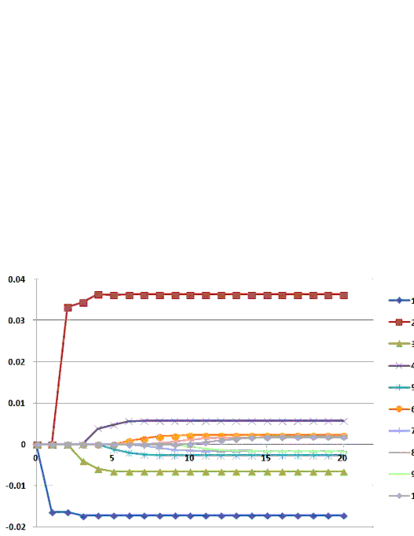
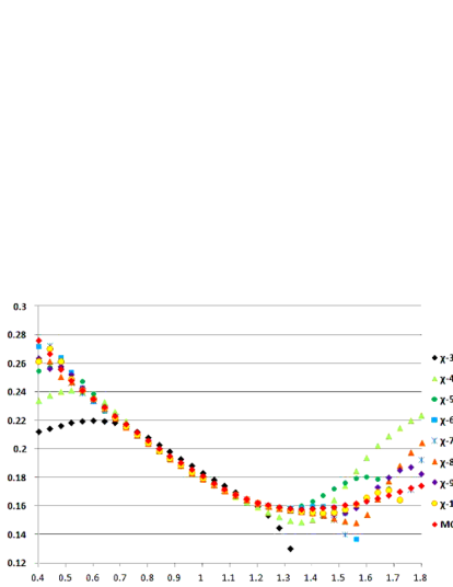
Figure 1: Estimation of moments and implied volatilities. $T=1,\sigma=0.15,\alpha=0.6,\rho=-0.6,\kappa=0.1,\mu_{J}=-0.02,\sigma_{J}=0.03$ and $\lambda(t,Y_{t})=8(Y_{t}+1)^{2}$.

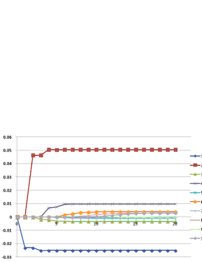
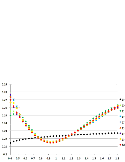
Figure 2: Estimation of moments and implied volatilities. $T=1,\sigma=0.15,\alpha=0.6,\rho=0,\kappa=0.1,\mu_{J}=-0.02,\sigma_{J}=0.03$ and $\lambda(t,Y_{t})=8(Y_{t}+1)^{2}$.

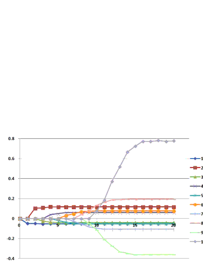
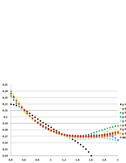
Figure 3: Estimation of moments and implied volatilities. $T=3,\sigma=0.15,\alpha=0.5,\rho=-0.5,\kappa=0.1,\mu_{J}=0.01,\sigma_{J}=0.035$ and $\lambda(t,Y_{t})=5Y_{t}^{2}+10Y_{t}+8$.

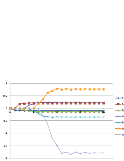
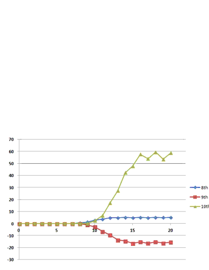
Figure 4: Estimation of moments. $T=5,\sigma=0.15,\alpha=0.5,\rho=-0.5,\kappa=0.1,\mu_{J}=0.01,\sigma_{J}=0.035$ and $\lambda(t,Y_{t})=5Y_{t}^{2}+10Y_{t}+8$.

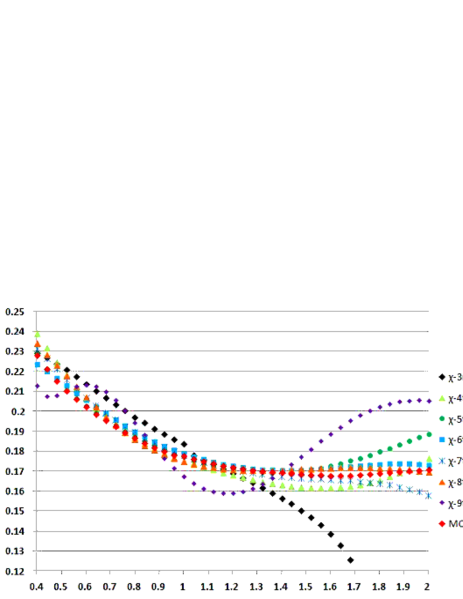
Figure 5: Estimation of implied volatilities. $T=5,\sigma=0.15,\alpha=0.5,\rho=-0.5,\kappa=0.1,\mu_{J}=0.01,\sigma_{J}=0.035$ and $\lambda(t,Y_{t})=5Y_{t}^{2}+10Y_{t}+8$.

Before closing this section, let us study the path-wise nature of the current approximation scheme for the terminal condition $H(X_{T})=X_{T}^{m}$. For each order of moment $m$ and expansion $n$, one can calculate the path-wise truncated approximation error $[X_{T}^{m}-\widetilde{V}^{(n)}_{T}]$, where $\widetilde{V}^{(n)}$ is given by (2.13) appropriately specified for the current model. In Figure 6, we have shown the scattered plot of this quantity for ($m=1$ and $5$) with various orders of expansion $n$ using the same setup as in Figure 3, i.e. $\{T=3,\sigma=0.15,\alpha=0.5,\rho=-0.5,\kappa=0.1,\mu_{J}=0.01,\sigma_{J}=0.035$ and $\lambda(t,Y_{t})=5Y_{t}^{2}+10Y_{t}+8\}$. In Table 1, the mean and standard deviation of $[X_{T}^{m}-\widetilde{V}^{(n)}_{T}]$ are given for $m=\{1,2,\cdots,5\}$ in the same setup. For ease of comparison, $\mathbb{E}[X_{T}^{m}]$ estimated by simulation is also given in the lower table for each moment. Note that the non-trivial approximation exists only for $n\geq m$. Improvement of approximation stops effectively at just a few higher order expansion $n\geq m$, which means that the contributions of polynomial expansion for the target of $X_{T}^{m}$ is dominated by $m$-th and just a couple of higher order polynomials. This is rather natural and also consistent with the left panel of Figure 3 showing the convergence of approximation series for each moment.

One can observe that our scheme can provide accurate path-wise approximation of $X^{m}$ but its error grows gradually for the higher moments. This fact can be naturally expected, since the contribution from the small number of realizations which reside in the tails of the distribution of $X_{T}$ becomes more important for higher moments. For the above example, the situation does not change meaningfully even if we use the pure diffusion model by putting $\lambda=0$. We have observed a minor improvement of convergence only by a factor of few. Since we have used the standard Euler scheme, the corresponding simulation error may be contributing to the above result to some extent.

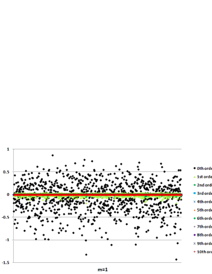
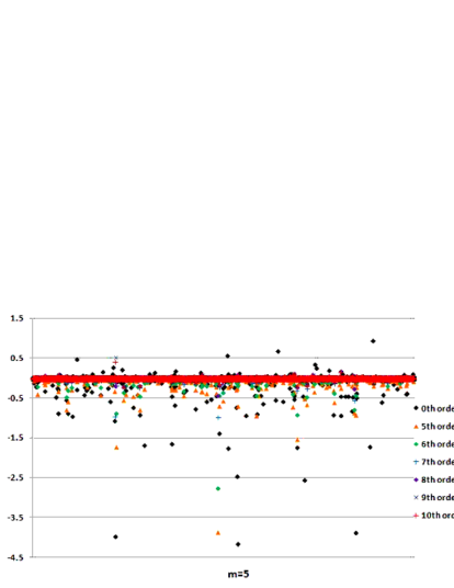
Figure 6: Scattered plot of $[X_{T}^{m}-\widetilde{V}^{(n)}_{T}]$ ($m=1$ in the left and $m=5$ in the right) with various expansion orders $n$. The setup is the same as in Figure 3.

$m=1$	$n=0$	$n=1$	$n=2$	$n=3$	$n=5$	$n=7$	$n=10$
mean	-0.054	$-3.4\times 10^{-3}$	$-3.2\times 10^{-3}$	$6.7\times 10^{-4}$	$1.4\times 10^{-5}$	$1.6\times 10^{-7}$	$1.5\times 10^{-6}$
stdev	0.34	0.028	$4.6\times 10^{-3}$	$9.5\times 10^{-4}$	$1.3\times 10^{-4}$	$1.2\times 10^{-4}$	$1.2\times 10^{-4}$
$m=2$	$n=0$	$n=2$	$n=3$	$n=4$	$n=5$	$n=7$	$n=10$
mean	0.12	0.014	$7.7\times 10^{-3}$	$-1.6\times 10^{-3}$	$1.9\times 10^{-4}$	$-4.7\times 10^{-5}$	$-5.4\times 10^{-5}$
stdev	0.22	0.044	0.017	$4.7\times 10^{-3}$	$3.9\times 10^{-3}$	$3.9\times 10^{-3}$	$3.9\times 10^{-3}$
$m=3$	$n=0$	$n=3$	$n=4$	$n=5$	$n=6$	$n=7$	$n=10$
mean	-0.041	-0.017	$-6.6\times 10^{-3}$	$4.7\times 10^{-4}$	$-1.8\times 10^{-4}$	$1.5\times 10^{-4}$	$3.9\times 10^{-5}$
stdev	0.27	0.084	0.043	$5.6\times 10^{-3}$	$5.3\times 10^{-3}$	$5.3\times 10^{-3}$	$5.2\times 10^{-3}$
$m=4$	$n=0$	$n=4$	$n=5$	$n=6$	$n=7$	$n=8$	$n=10$
mean	0.060	0.025	0.014	$8.3\times 10^{-4}$	$6.1\times 10^{-4}$	$-4.4\times 10^{-4}$	$-1.2\times 10^{-4}$
stdev	0.39	0.18	0.11	0.019	0.012	0.011	0.010
$m=5$	$n=0$	$n=5$	$n=6$	$n=7$	$n=8$	$n=9$	$n=10$
mean	-0.050	-0.037	-0.021	$-5.2\times 10^{-3}$	$-1.9\times 10^{-3}$	$6.8\times 10^{-4}$	$-9.0\times 10^{-6}$
stdev	0.65	0.40	0.28	0.084	0.042	0.025	0.024

	$m=1$	$m=2$	$m=3$	$m=4$	$m=5$
$\mathbb{E}[X_{T}^{m}]$	$-5.60\times 10^{-2}$	$1.16\times 10^{-1}$	$-4.30\times 10^{-2}$	$6.33\times 10^{-2}$	$-5.69\times 10^{-2}$

Table 1: Mean and standard deviation of the path-wise realizations of $[X_{T}^{m}-\widetilde{V}^{(n)}_{T}]$ of $m=\{1,\cdots,5\}$ with the same setup as in Figure 3 by simulation. The second table gives the figures of $\mathbb{E}[X_{T}^{m}]$ with $m=\{1,\cdots,5\}$ estimated by MC simulation for clarity.

4 An Application to $\lambda$-SABR Model

4.1 Problem Setup

By using an appropriate change of variables, the proposed polynomial expansion scheme can be applied to a wider choice of models than what may be naively imagined. Let us consider (rescaled) $\lambda$-SABR model (SABR model with mean-reverting volatility) under an equivalent martingale measure $\mathbb{Q}$.

$$S_{t}=S_{0}+\int_{0}^{t}(S_{0}^{1-\beta})\sigma(s)\bar{Y}_{s}S_{s}^{\beta}dW_{s}$$ (4.1)

$$\bar{Y}_{t}=1+\int_{0}^{t}\Bigl{(}\alpha(s)\bar{Y}_{s}dB_{s}+\kappa(s)(1-\bar{Y}_{s})ds\Bigr{)}$$ (4.2)

where $W$, $B$ are one-dimensional $\mathbb{Q}$-Brownian motions with $d\langle W,B\rangle_{t}=\rho(t)dt$. $(\sigma,\rho,\kappa)$ are all deterministic functions, and $\beta\in[0,1)$ is a constant. Here, a factor of $S_{0}^{1-\beta}$ is included to make $\sigma$ roughly equal to the at-the-money implied volatility of $S$.

The change of variables

$$X_{t}:=\frac{1}{1-\beta}\left(\Bigl{(}\frac{S_{t}}{S_{0}}\Bigr{)}^{1-\beta}-1\right)$$ (4.3)

$$Y_{t}:=\bar{Y}_{t}-1$$ (4.4)

leads to the dynamics

$$X_{t}=\int_{0}^{t}\left(\sigma(s)(1+Y_{s})dW_{s}-\frac{\beta}{2}\sigma(s)^{2}b(X_{s})(1+Y_{s})^{2}ds\right)$$ (4.5)

$$Y_{t}=\int_{0}^{t}\Bigl{(}\alpha(s)(1+Y_{s})dB_{s}-\kappa(s)Y_{s}ds\Bigr{)}$$ (4.6)

where

$$b(x):=\frac{1}{1+(1-\beta)x}~{}.$$ (4.7)

The assumption on the quadratic covariation (2.4) is now satisfied for these new variables.

The BSDE relevant for a European contingent claim with terminal payoff $H(X_{T})$ at maturity $T$ is given by

$$V_{t} = H(X_{T})-\int_{t}^{T}\left(\frac{\beta}{2}\sigma(s)^{2}b(X_{s})(1+Y_{s})^{2}Z_{s}+\kappa(s)Y_{s}\Gamma_{s}\right)ds$$ (4.8)

$$-\int_{t}^{T}Z_{s}dX_{s}-\int_{t}^{T}\Gamma_{s}dY_{s}$$

As in the Heston’s case, we choose $H(x)=x^{m},~{}(m=1,2,\cdots)$ to obtain the moment estimate of $X_{T}$ and then use the Edgeworth expansion to approximate its probability density. Here, we are not claiming the Edgeworth expansion is the best choice and different basis functions (such as Laguerre polynomials) can be more appropriate.

4.2 Polynomial Expansion

We now introduce $\epsilon$ to the BSDE (4.8) so that we can perform polynomial expansion

$$V_{t}^{\epsilon} = H(\epsilon X_{T})-\int_{t}^{T}\left(\frac{\beta}{2}\sigma(s)^{2}b(\epsilon X_{s})(1+\epsilon Y_{s})^{2}Z_{s}^{\epsilon}+\epsilon\kappa(s)Y_{s}\Gamma_{s}^{\epsilon}\right)ds$$ (4.9)

$$-\int_{t}^{T}Z_{s}^{\epsilon}dX_{s}-\int_{t}^{T}\Gamma_{s}^{\epsilon}dY_{s}$$

as

$$V_{t}^{\epsilon}=\sum_{n=0}^{\infty}\epsilon^{n}V_{t}^{[n]}$$ (4.10)

$$Z_{t}^{\epsilon}=\sum_{n=0}^{\infty}\epsilon^{n}Z_{t}^{[n]},\quad\Gamma_{t}^{\epsilon}=\sum_{n=0}^{\infty}\epsilon^{n}\Gamma_{t}^{[n]}~{}.$$ (4.11)

We have the following lemma.

Lemma 2

If it exists, the polynomial solution for the expansion in (4.10) and (4.11) is uniquely given by

$$V_{t}^{[n]}=\sum_{m=0}^{n}\sum_{k=0}^{m}\frac{X_{t}^{m-k}Y_{t}^{k}}{(m-k)!k!}v^{[n]}_{m-k,k}(t)$$ (4.12)

$$Z_{t}^{[n]}=\sum_{m=1}^{n}\sum_{k=0}^{m-1}\frac{X_{t}^{m-k-1}Y_{t}^{k}}{(m-k-1)!k!}v^{[n]}_{m-k,k}(t)$$ (4.14)

$$\Gamma_{t}^{[n]}=\sum_{m=1}^{n}\sum_{k=1}^{m}\frac{X_{t}^{m-k}Y_{t}^{k-1}}{(m-k)!(k-1)!}v^{[n]}_{m-k,k}(t)$$

with the set of deterministic functions $v^{[n]}_{m-k,k}(t)$ of $(0\leq k\leq m\leq n)$ satisfying the following recursive system of linear ODEs

$$\dot{v}^{[n]}_{m-k,k}(t)=-\mathbb{I}_{(2\leq k)}k(k-1)\left(\frac{\sigma_{t}^{2}}{2}v^{[n]}_{m-k+2,k-2}(t)+\rho_{t}\sigma_{t}\alpha_{t}v^{[n]}_{m-k+1,k-1}(t)+\frac{\alpha_{t}^{2}}{2}v^{[n]}_{m-k,k}(t)\right)$$

$$\quad-\mathbb{I}_{(m\leq n-1,1\leq k)}k\Bigl{(}\sigma_{t}^{2}v^{[n]}_{m-k+2,k-1}(t)+2\rho_{t}\sigma_{t}\alpha_{t}v^{[n]}_{m-k+1,k}(t)+\alpha_{t}^{2}v^{[n]}_{m-k,k+1}(t)\Bigr{)}$$

$$\quad-\mathbb{I}_{(m\leq n-2)}\left(\frac{\sigma_{t}^{2}}{2}v^{[n]}_{m-k+2,k}(t)+\rho_{t}\sigma_{t}\alpha_{t}v^{[n]}_{m-k+1,k+1}(t)+\frac{\alpha_{t}^{2}}{2}v^{[n]}_{m-k,k+2}(t)\right)$$

$$\quad+\mathbb{I}_{(m\leq n-1,1\leq k)}k\kappa_{t}v^{[n-1]}_{m-k,k}(t)+\mathbb{I}_{(m\leq n-1)}\frac{\beta}{2}\sigma_{t}^{2}\sum_{l=0}^{m-k}C(m-k,l)\partial^{l}_{x}b(0)\times$$

$$\quad\left(v^{[n-l]}_{m-k-l+1,k}(t)+\mathbb{I}_{(1\leq k)}2k~{}v^{[n-l-1]}_{m-k-l+1,k-1}(t)+\mathbb{I}_{(2\leq k)}k(k-1)~{}v^{[n-l-2]}_{m-k-l+1,k-2}(t)\frac{\bigl{.}}{}\right)$$

(4.15)

having the terminal conditions $v^{[n]}_{n,0}(T)=\partial_{x}^{n}H(0)$ with all the other components zero.

Proof: It can be proved in exactly the same way as Lemma 1. The derivation is given in the Appendix A.

4.3 Numerical Examples

As in Section 3.4, let us provide several numerical examples for the estimated moments and the comparison of the implied volatilities. The number of paths for Monte-Carlo simulation is $500,000$ as before. For this model, we cannot use the special relation in (3.32) and (3.33), and hence we have carried out numerical integration of the estimated density for the pricing. The styles and conventions used in each figures are the same as those in Section 3.4.

Although the polynomial expansion gives similar accuracy for short maturities, its applicability to long maturities is rather limited compared to the previous extended Heston model. The main cause seems to be the factor $k(k-1)$ appearing in the first line of the ODE given in Lemma 2, which strongly drives $\{v^{[n]}_{m,k}\}$ especially for higher moments and makes them unable to converge. This factor stems from the terms $\propto Y^{2}$ in the quadratic covariations. In addition, since the support of $X_{t}$ is limited to the range $X_{t}\geq-\displaystyle{\frac{1}{1-\beta}}$, the model’s compatibility to the Edgeworth expansion may be lower than the Heston model. This may be one of the reasons for somewhat unstable behavior of the implied volatilities when higher-order cumulants are included.

For completeness, we give a convergence analysis for the path-wise realizations of the truncated approximation $[X_{T}^{m}-\widetilde{V}^{(n)}_{T}]$ as before. In Table 2, the mean and standard deviation for $m=\{1,2,\cdots,5\}$ with various order of expansions are given under the same setup used in Figure 8. In this model, the improvement of approximation stops more quickly than the previous Heston model case. This is likely due to the smaller size of moments  and possibly other delicate model features. The quicker convergence of approximation series can also be seen from the left panel of Figure 8.

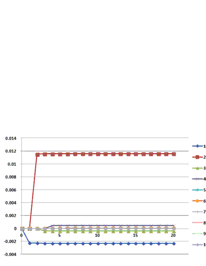
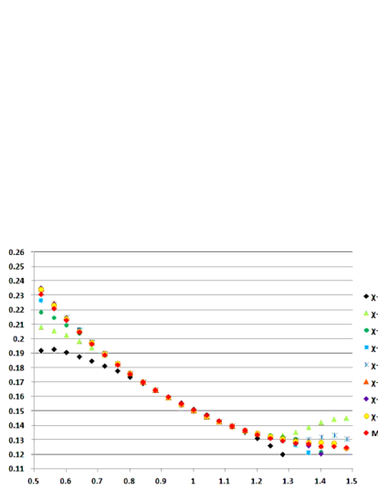
Figure 7: Estimation of moments and implied volatilities. $T=0.5,\sigma=0.15,\alpha=0.3,\rho=-0.4,\kappa=0.1,\beta=0.4$.

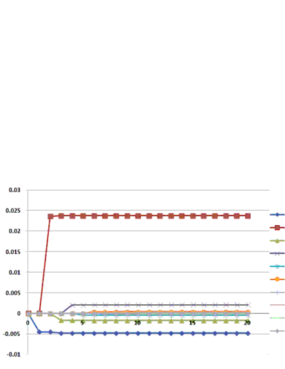
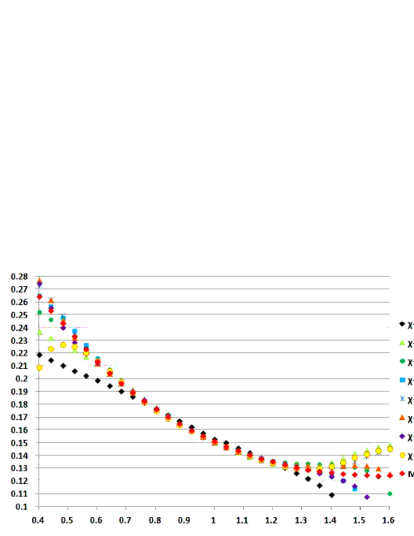
Figure 8: Estimation of moments and implied volatilities. $T=1,\sigma=0.15,\alpha=0.3,\rho=-0.4,\kappa=0.1,\beta=0.4$.

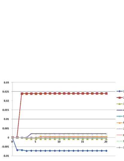
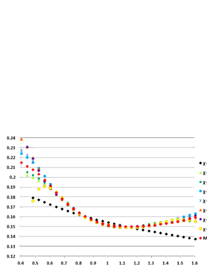
Figure 9: Estimation of moments and implied volatilities. $T=1,\sigma=0.15,\alpha=0.35,\rho=0,\kappa=0.1,\beta=0.6$.

$m=1$	$n=0$	$n=1$	$n=2$	$n=3$	$n=5$	$n=7$	$n=10$
mean	$-4.7\times 10^{-3}$	$-2.8\times 10^{-4}$	$-2.7\times 10^{-4}$	$1.8\times 10^{-6}$	$-4.4\times 10^{-7}$	$5.5\times 10^{-8}$	$1.0\times 10^{-7}$
stdev	0.15	$1.9\times 10^{-3}$	$4.1\times 10^{-4}$	$7.5\times 10^{-5}$	$1.8\times 10^{-5}$	$1.7\times 10^{-5}$	$1.7\times 10^{-5}$
$m=2$	$n=0$	$n=2$	$n=3$	$n=4$	$n=5$	$n=7$	$n=10$
mean	0.024	$2.1\times 10^{-4}$	$5.3\times 10^{-5}$	$2.2\times 10^{-5}$	$1.2\times 10^{-5}$	$1.1\times 10^{-5}$	$1.0\times 10^{-5}$
stdev	0.037	$1.3\times 10^{-3}$	$1.2\times 10^{-3}$	$1.2\times 10^{-3}$	$1.2\times 10^{-3}$	$1.2\times 10^{-3}$	$1.2\times 10^{-3}$
$m=3$	$n=0$	$n=3$	$n=4$	$n=5$	$n=6$	$n=7$	$n=10$
mean	$-1.6\times 10^{-3}$	$-4.0\times 10^{-5}$	$-4.1\times 10^{-5}$	$-5.7\times 10^{-6}$	$-3.0\times 10^{-6}$	$-1.8\times 10^{-6}$	$-1.4\times 10^{-6}$
stdev	0.018	$6.5\times 10^{-4}$	$5.9\times 10^{-4}$	$5.6\times 10^{-4}$	$5.6\times 10^{-4}$	$5.6\times 10^{-4}$	$5.6\times 10^{-4}$
$m=4$	$n=0$	$n=4$	$n=5$	$n=6$	$n=7$	$n=8$	$n=10$
mean	$1.9\times 10^{-3}$	$2.6\times 10^{-5}$	$2.1\times 10^{-5}$	$7.9\times 10^{-6}$	$5.4\times 10^{-6}$	$4.7\times 10^{-6}$	$4.4\times 10^{-6}$
stdev	$9.1\times 10^{-3}$	$4.8\times 10^{-4}$	$4.5\times 10^{-4}$	$4.3\times 10^{-4}$	$4.3\times 10^{-4}$	$4.3\times 10^{-4}$	$4.3\times 10^{-4}$
$m=5$	$n=0$	$n=5$	$n=6$	$n=7$	$n=8$	$n=9$	$n=10$
mean	$-3.8\times 10^{-4}$	$-9.7\times 10^{-6}$	$-1.4\times 10^{-6}$	$-4.6\times 10^{-6}$	$-3.4\times 10^{-6}$	$-2.9\times 10^{-6}$	$-2.7\times 10^{-6}$
stdev	$5.7\times 10^{-3}$	$3.9\times 10^{-4}$	$3.7\times 10^{-4}$	$3.6\times 10^{-4}$	$3.5\times 10^{-4}$	$3.5\times 10^{-4}$	$3.6\times 10^{-4}$

	$m=1$	$m=2$	$m=3$	$m=4$	$m=5$
$\mathbb{E}[X_{T}^{m}]$	$-4.78\times 10^{-3}$	$2.39\times 10^{-2}$	$-1.73\times 10^{-3}$	$2.04\times 10^{-3}$	$-4.48\times 10^{-4}$

Table 2: Mean and standard deviation of the path-wise realizations of $[X_{T}^{m}-\widetilde{V}^{(n)}_{T}]$ of $m=\{1,\cdots,5\}$ with the setup in Figure 8 by simulation. The second table gives the figures of $\mathbb{E}[X_{T}^{m}]$ with $m=\{1,\cdots,5\}$ estimated by MC simulation for clarity.

5 Utility Optimization with Terminal Liability

European contingent claims, which we studied in the previous sections, can of course be solved without resorting to a complicated BSDE formulation. The main motivation there was to get some insight about the performance of the proposed scheme by studying the two popular models. Now, in this section, we treat a utility-optimization problem in an incomplete market where solving a BSDE becomes crucially important.

Here, we adopt a simple Heston security market consists of one-risky asset with stochastic volatility. For simplicity, we assume that the interest rate is zero. In the probability space of the physical measure $(\Omega,{\cal F},\mathbb{P})$, the dynamics of the underlying variables is assumed to be given by

$$S_{t}=S_{0}+\int_{0}^{t}S_{s}\sigma(s)\sqrt{\bar{Y}_{s}}\Bigl{(}dW_{s}+\bar{\theta}(s,S_{s},\bar{Y}_{s})ds\Bigr{)}$$

$$\bar{Y}_{t}=1+\int_{0}^{t}\left(\frac{\bigl{.}}{\bigr{.}}\alpha(s)\sqrt{\bar{Y}_{s}}\Bigl{(}dB_{s}+\rho(s)\bar{\theta}(s,S_{s},\bar{Y}_{s})ds\Bigr{)}+\kappa(s)(1-\bar{Y}_{s})ds\right)$$ (5.1)

where $W,B$ are $\mathbb{P}$-Brownian motions with $d\langle W,B\rangle_{t}=\rho(t)dt$. $\sigma,\alpha$ and $\kappa$ are deterministic functions of time, and $\bar{\theta}:[0,T]\times\mathbb{R}_{+}^{2}\rightarrow\mathbb{R}$ gives the risk-premium process associating with $W$. The risk-premium for $B$ is implied by the $\rho\bar{\theta}$ as well as the mean-reverting term of $\bar{Y}$.

Given a portfolio strategy $(\pi_{t})_{t\geq 0}$, the wealth at the terminal time $T~{}(>t)$ is given by

$${\cal W}^{\pi}_{T}(t,w)=w+\int_{t}^{T}\pi_{u}dS_{u}~{}.$$ (5.2)

In the reminder of this section, we are going to study the BSDE associated with the exponential cost minimization:

$$V(t,w)={\rm ess}\inf_{\pi}\mathbb{E}\left[\exp\left(\frac{\bigl{.}}{}\gamma\Bigl{(}\bar{H}(S_{T},Y_{T})-{\cal W}_{T}^{\pi}(t,w)\Bigr{)}\right)\Bigr{|}{\cal F}_{t}\right]$$ (5.3)

where $\gamma$ is a positive constant specifying the risk averseness, and $\bar{H}:\mathbb{R}_{+}^{2}\rightarrow\mathbb{R}$ is a smooth function denoting the terminal liability. Using Itô-Ventzell formula and the transformation

$$V(t)=\ln\Bigl{(}V(t,w)e^{\gamma w}\Bigr{)}$$ (5.4)

one can show that the following BSDE holds:

$$V_{t}=\gamma\bar{H}(S_{T},\bar{Y}_{T})-\int_{t}^{T}\left\{\frac{1}{2}\bar{\theta}(s,S_{s},\bar{Y}_{s})^{2}-\frac{1}{2}(1-\rho(s)^{2})\bar{\Gamma}_{s}^{2}\right\}ds$$

$$\quad-\int_{t}^{T}\bar{Z}_{s}\Bigl{[}dW_{s}+\bar{\theta}(s,S_{s},\bar{Y}_{s})ds\Bigr{]}-\int_{t}^{T}\bar{\Gamma}_{s}\Bigl{[}dB_{s}+\rho(s)\bar{\theta}(s,S_{s},\bar{Y}_{s})ds\Bigr{]}~{}.$$ (5.5)

It is well-known that the transformation (5.4) makes $V(t)$ independent from the initial wealth $w$. The details and various interesting topics can be found in a comprehensive review by Mania & Tevzadze (2008) [28]. Similar qgBSDE arises in other economically important setups too, such as Power and HARA (hyperbolic absolute risk aversion) utilities after appropriate change of variables. We simply study (5.5) for a demonstrative purpose of the current approximation scheme.

It is important to notice that one cannot make use of Cole-Hopf transformation to convert the qgBSDE (5.5) to a solvable linear BSDE as long as $(\bar{H},\bar{\theta})$ depend on both of the $S$ and $\bar{Y}$. For example, if both of them depend only on $\bar{Y}$, one can solve it analytically by following the arguments given by Zariphopoulou (2001) [37].

As in Section 3, we perform the change of variables

$$X_{t}=\ln\left(\frac{S_{t}}{S_{0}}\right)$$ (5.6)

$$Y_{t}=\bar{Y}_{t}-1$$ (5.7)

and define

$$\theta(s,X_{s},Y_{s}):=\bar{\theta}(s,S_{s},\bar{Y}_{s})~{}.$$ (5.8)

The relevant forward SDEs are now given by

$$X_{t}=\int_{0}^{t}\left\{\sigma(s)\sqrt{Y_{s}+1}\Bigl{(}dW_{s}+\theta(s,X_{s},Y_{s})ds\Bigr{)}-\frac{\sigma(s)^{2}}{2}(Y_{s}+1)ds\frac{\bigl{.}}{}\right\}$$ (5.9)

$$Y_{t}=\int_{0}^{t}\left\{\alpha(s)\sqrt{Y_{s}+1}\Bigl{(}dB_{s}+\rho(s)\theta(s,X_{s},Y_{s})ds\Bigr{)}-\kappa(s)Y_{s}ds\frac{\bigl{.}}{}\right\}~{}.$$ (5.10)

Simple redefinition of variables yields

$$V_{t}=\gamma H(X_{T},Y_{T})-\int_{t}^{T}Z_{s}dX_{s}-\int_{t}^{T}\Gamma_{s}dY_{s}-\int_{t}^{T}\left\{\frac{1}{2}\Theta(s,X_{s},Y_{s})\right.$$

$$\qquad\left.-\frac{\alpha(s)^{2}}{2}(1-\rho(s)^{2})(1+Y_{s})\Gamma_{s}^{2}+\frac{\sigma(s)^{2}}{2}(1+Y_{s})Z_{s}+\kappa(s)Y_{s}\Gamma_{s}\right\}ds$$ (5.11)

where $H(X_{T},Y_{T}):=\bar{H}(S_{T},\bar{Y}_{T})$ and $\Theta(s,X_{s},Y_{s})=\theta(s,X_{s},Y_{s})^{2}$ . The control variables are connected to those in (5.5) by

$$\bar{Z}_{s}=Z_{s}\sigma(s)\sqrt{Y_{s}+1},\quad\bar{\Gamma}_{s}=\Gamma_{s}\alpha(s)\sqrt{Y_{s}+1}~{}.$$ (5.12)

We assume the system of the forward and backward SDEs (5.9), (5.10) and (5.11) has a well-posed solution in the reminder of the section. Although it deviates from the main subject of the paper, it is interesting to notice that the above BSDE has a simple exact solution in a special case. The details are give in Appendix C.

5.1 Polynomial Expansion

In order to obtain the polynomial approximation for the system (5.9), (5.10) and (5.11), let us introduce $\epsilon$ and consider the perturbed BSDE:

$$V_{t}^{\epsilon}=\gamma H(\epsilon X_{T},\epsilon Y_{T})-\int_{t}^{T}Z_{s}^{\epsilon}dX_{s}-\int_{t}^{T}\Gamma_{s}^{\epsilon}dY_{s}-\int_{t}^{T}\left\{\frac{\bigl{.}}{}\frac{1}{2}\Theta(s,\epsilon X_{s},\epsilon Y_{s})\right.$$

$$\quad\left.-\frac{\alpha(s)^{2}}{2}(1-\rho(s)^{2})(1+\epsilon Y_{s})[\Gamma_{s}^{\epsilon}]^{2}+\frac{\sigma(s)^{2}}{2}(1+\epsilon Y_{s})Z_{s}^{\epsilon}+\epsilon\kappa(s)Y_{s}\Gamma_{s}^{\epsilon}\frac{\bigl{.}}{}\right\}ds$$ (5.13)

and the associated expansion

$$V_{t}^{\epsilon}=\sum_{n=0}^{\infty}\epsilon^{n}V_{t}^{[n]}$$ (5.14)

$$Z_{t}^{\epsilon}=\sum_{n=0}^{\infty}\epsilon^{n}Z_{t}^{[n]},\qquad\Gamma_{t}^{\epsilon}=\sum_{n=0}^{\infty}\epsilon^{n}\Gamma_{t}^{[n]}~{}.$$ (5.15)

The approximate solution of the original system is obtained by truncating the summation at a certain order $n$ and putting $(\epsilon=1)$ as explained in Section 2.2. For this model, we have the following result:

Lemma 3

If it exists, the polynomial solution for the expansion in (5.14) and (5.15) is uniquely given by

$$V_{t}^{[n]}=\sum_{m=0}^{n}\sum_{k=0}^{m}\frac{X_{t}^{m-k}Y_{t}^{k}}{(m-k)!k!}v^{[n]}_{m-k,k}(t)$$ (5.16)

$$Z_{t}^{[n]}=\sum_{m=1}^{n}\sum_{k=0}^{m-1}\frac{X_{t}^{m-k-1}Y_{t}^{k}}{(m-k-1)!k!}v^{[n]}_{m-k,k}(t)$$ (5.17)

$$\Gamma_{t}^{[n]}=\sum_{m=1}^{n}\sum_{k=1}^{m}\frac{X_{t}^{m-k}Y_{t}^{k-1}}{(m-k)!(k-1)!}v^{[n]}_{m-k,k}(t)$$ (5.18)

with the set of deterministic functions $v^{[n]}_{m-k,k}(t)$ of $(0\leq k\leq m\leq n)$ satisfying the following recursive system of linear ODEs

$$\dot{v}^{[n]}_{m-k,k}(t)=-\mathbb{I}_{(m\leq n-1,1\leq k)}k\left(\frac{\sigma_{t}^{2}}{2}v^{[n]}_{m-k+2,k-1}(t)+\rho_{t}\sigma_{t}\alpha_{t}v^{[n]}_{m-k+1,k}(t)+\frac{\alpha_{t}^{2}}{2}v^{[n]}_{m-k,k+1}(t)\right)$$

$$-\mathbb{I}_{(m\leq n-2)}\left(\frac{\sigma_{t}^{2}}{2}v^{[n]}_{m-k+2,k}(t)+\rho_{t}\sigma_{t}\alpha_{t}v^{[n]}_{m-k+1,k+1}(t)+\frac{\alpha_{t}^{2}}{2}v^{[n]}_{m-k,k+2}(t)\right)$$

$$+\mathbb{I}_{(m=n)}\frac{1}{2}\partial_{x}^{n-k}\partial_{y}^{k}\Theta(t,0,0)+\mathbb{I}_{(m\leq n-1)}\frac{\sigma_{t}^{2}}{2}v^{[n]}_{m-k+1,k}(t)$$

$$+\mathbb{I}_{(m\leq n-1,1\leq k)}k\left(\frac{\sigma_{t}^{2}}{2}v^{[n-1]}_{m-k+1,k-1}(t)+\kappa_{t}v^{[n-1]}_{m-k,k}(t)\right)$$

$$-\mathbb{I}_{(m\leq n-2)}\sum_{l=1}^{n-1}\sum_{j=1\vee[l+2-n+m]}^{l\wedge[m+1]}\sum_{p=1\vee[j-m+k]}^{j\wedge[k+1]}\frac{\alpha_{t}^{2}}{2}\xi_{t}^{2}C_{(m-k,j-p)}C_{(k,p-1)}v^{[l]}_{j-p,p}(t)v^{[n-l]}_{m-k-j+p,k-p+2}(t)$$

$$-\mathbb{I}_{(1\leq m\leq n-2,1\leq k)}\sum_{l=1}^{n-2}\sum_{j=1\vee[l+2-n+m]}^{l\wedge m}\sum_{p=1\vee[j-m+k]}^{j\wedge k}\frac{\alpha_{t}^{2}}{2}\xi_{t}^{2}C_{(m-k,j-p)}C_{(k,p)}pv^{[l]}_{j-p,p}(t)v^{[n-l-1]}_{m-k-j+p,k-p+1}(t)$$

with $\xi_{t}^{2}:=(1-\rho(t)^{2})$ and the terminal conditions $v^{[n]}_{n-k,k}(T)=\gamma\partial_{x}^{n-k}\partial_{y}^{k}H(0,0)$ with all the other components zero.

Proof: The proof is done in a similar way to Lemma 1 and 2. The details of the derivation are given in Appendix B.

5.2 Numerical Examples

For numerical examples, we shall use

$$\Theta(t,X_{t},Y_{t}):=c_{0}e^{-c_{1}X_{t}}(Y_{t}+1)$$ (5.20)

$$H(X_{T},Y_{T}):=e^{-g_{1}X_{T}}G(Y_{T})$$ (5.21)

where $c_{0},c_{1},g_{1}$ are constants and $G(\cdot)$ a smooth function of $Y$. Since the parameter of risk-averseness $\gamma$ appears only in a combination $\gamma H$, the factor $e^{-g_{1}X_{T}}$ can equivalently be interpreted as a $S_{T}$-dependent risk averseness.

The problem analyzed in this section is intrinsically non-linear. Thus, we cannot use the density approximation and must directly approximate the terminal payoff by a smooth function. In practice, however, it should not be a prohibitive limitation. Since the problem is non-linear, one has to consider the optimization in a portfolio level. Then, considering an appropriate hedging strategy based on a smooth approximate payoff function, instead of treating it exactly, should be reasonable.

We consider the next four choices of terminal liability (except $e^{-g_{1}x}$ factor) in the numerical examples:

$$(1):~{}\sin\Bigl{(}y+\frac{\pi}{6}\Bigr{)}$$ (5.22)

$$(2):~{}\max\bigl{(}0,y\bigr{)}$$ (5.23)

$$(3):~{}\max\bigl{(}0,-y\bigr{)}$$ (5.24)

$$(4):~{}0.6-\max\bigl{(}0,0.2-y\bigr{)}$$ (5.25)

For $(2)$ to $(4)$, we have approximated it by a $5$th-order polynomial function determined by a simple least-square method, and treat it as the true $G(y)$ in the evaluation. Here, the shapes of the liability and the order of approximating polynomial function are chosen rather arbitrary. In practice, one has to consider in a portfolio level and needs to choose a certain order of polynomial to recover its overall shape. The impact from adding another term would be easy to check directly. It is naturally expected, however, that the higher order terms plays only a minor role otherwise it means that the firm is taking quite problematic positions and exposing it to the far-tail behavior of the underlying securities.

Each of Figure 10 to 13 consists of: 1)Top left: a graph of $G(y)$, 2)Top right: a graph of the truncated value function and control variables $(V^{(n)}_{0},Z^{(n)}_{0},\Gamma^{(n)}_{0})$ for each $n$ specified by the horizontal axis , 3)Bottom left: a scattered plot of $[\gamma H(X_{T},Y_{T})-\widetilde{V}^{(n)}_{T}]$ for each expansion order, 4) Bottom right: a graph of the means as well as the standard deviations of $[\gamma H(X_{T},Y_{T})-\widetilde{V}_{T}^{(n)}]$ for $(0\leq n\leq 10)$ with 100,000-path simulation, whose details are also given in a table associated with each example. Note that the errors are measured relative to the smoothly modified terminal functions in $(2)$ to $(4)$ cases.

From the definition of the truncated approximation, one can easily see that the mean of $[\gamma H(X_{T},Y_{T})-\widetilde{V}^{(n)}_{T}]$ is equivalent to the estimate of

$$V_{0}^{(n)}-\mathbb{E}\left[\gamma H(X_{T},Y_{T})-\int_{0}^{T}Z_{t}^{(n)}dX_{t}-\int_{0}^{T}\Gamma_{t}^{(n)}dY_{t}\right.$$

$$\left.-\int_{0}^{T}\Bigl{\{}\frac{1}{2}\Theta(t,X_{t},Y_{t})-\frac{\alpha^{2}}{2}(1-\rho^{2})(1+Y_{t})[\Gamma_{t}^{(n)}]^{2}+\frac{\sigma^{2}}{2}(1+Y_{t})Z_{t}^{(n)}+\kappa Y_{t}\Gamma_{t}^{(n)}\Bigr{\}}dt\right]$$ (5.26)

by simulation. Its convergence to zero gives one consistency test for the value function at the initial point. The scattered plots of $[\gamma H(X_{T},Y_{T})-\widetilde{V}^{(n)}_{T}]$ and the corresponding standard deviations provide a much stronger test. They suggest that the truncated value functions and control variables give a good path-wise approximation for the original BSDE. One can clearly observe that the deviations $[\gamma H(X_{T},Y_{T})-\widetilde{V}^{(n)}_{T}]$ at the maturity are strongly clustering around zero even for a relatively low expansion order $n\sim 3$. Of course, as one can imagine, the probability that the size of $\bigl{(}\gamma H(X_{T},Y_{T}),X_{T},Y_{T}\bigr{)}$ becomes (meaningfully) bigger than one should be small enough in order to obtain a converging result. This means that we need to adopt a proper “scaling” for the wealth and the other parameters to make sure the chosen utility (or cost function) stays ${\cal O}(1)$ .

Remark

For those who have checked the result of Lemma 3 by themselves, it must be clear that deriving a closed form system of ODEs would be much harder in a realistic multi-asset setup. In that sense, the above numerical result is quite encouraging by implying that one may get a reasonable approximation even by a lower order expansion, for example, $n\sim 4$. In this case, step-by-step derivation of the relevant ODEs following the instruction given in Section 2.2 can be done without much difficulty even for a more involved BSDE. Interesting practical applications are left for the future research.

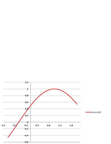
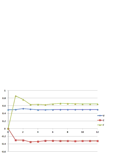
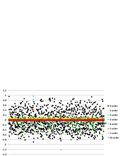
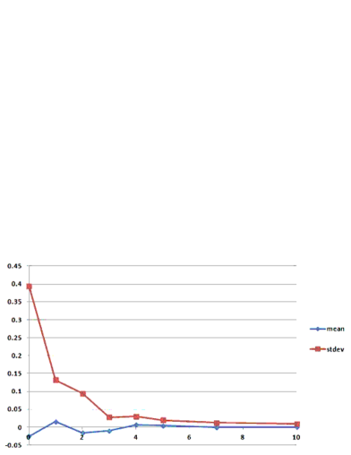
Figure 10: $T=1,\sigma=0.2,\alpha=0.5,\rho=-0.7,\kappa=0.1,c_{0}=0.01$, $c_{1}=0.4,\gamma=1,g_{1}=0.6$. $G(y)=\sin(y+\pi/6)$.

	$n=0$	$n=1$	$n=2$	$n=3$	$n=4$	$n=5$	$n=7$	$n=10$
mean	-0.026	0.016	-0.016	-0.011	$6.3\times 10^{-3}$	$3.9\times 10^{-3}$	$-6.5\times 10^{-4}$	$5.0\times 10^{-4}$
stdev	0.39	0.13	0.094	0.027	0.030	0.020	0.012	$9.1\times 10^{-3}$

Table 3: Mean and standard deviation of $[\gamma H_{T}-\widetilde{V}^{(n)}_{T}]$ for the setup in Figure 10.

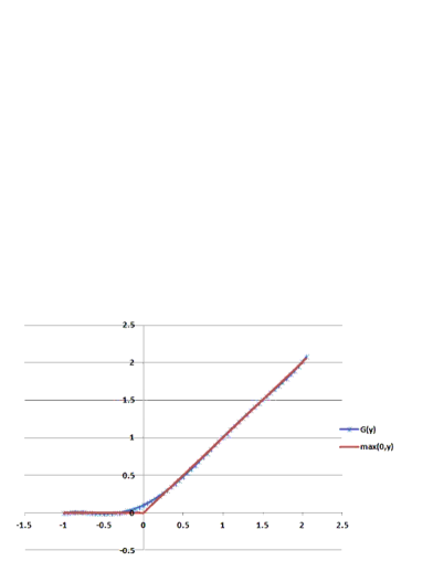
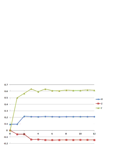
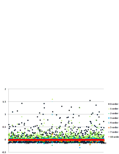
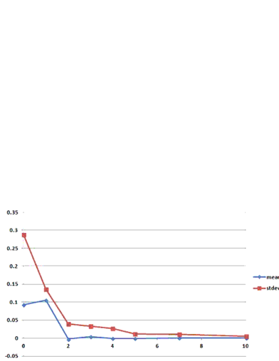
Figure 11: $T=1,\sigma=0.2,\alpha=0.4,\rho=-0.6,\kappa=0.1,c_{0}=0.01$, $c_{1}=0.4,\gamma=1,g_{1}=0.6$. $G(y)$ is a $5$-th order polynomial approximating $\max(0,y)$.

	$n=0$	$n=1$	$n=2$	$n=3$	$n=4$	$n=5$	$n=7$	$n=10$
mean	0.093	0.10	$-2.8\times 10^{-3}$	$3.7\times 10^{-3}$	$-8.2\times 10^{-4}$	$-1.3\times 10^{-3}$	$2.9\times 10^{-4}$	$1.3\times 10^{-4}$
stdev	0.29	0.14	0.040	0.030	0.026	0.011	0.011	$5.3\times 10^{-3}$

Table 4: Mean and standard deviation of $[\gamma H_{T}-\widetilde{V}^{(n)}_{T}]$ for the setup in Figure 11.

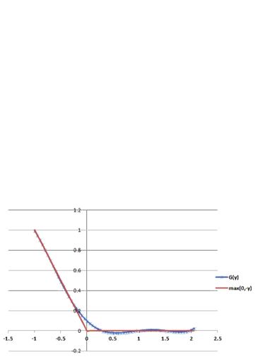
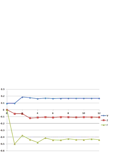
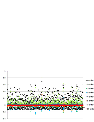
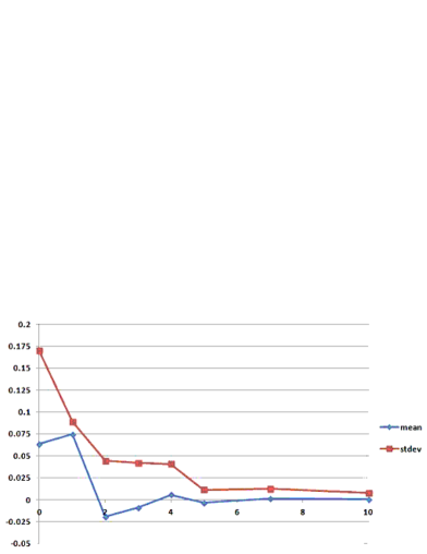
Figure 12: $T=1,\sigma=0.2,\alpha=0.4,\rho=-0.6,\kappa=0.1,c_{0}=0.01$, $c_{1}=0.4,\gamma=1,g_{1}=0.6$. $G(y)$ is a $5$-th order polynomial approximating $\max(0,-y)$.

	$n=0$	$n=1$	$n=2$	$n=3$	$n=4$	$n=5$	$n=7$	$n=10$
mean	0.064	0.075	-0.019	$-8.6\times 10^{-3}$	$5.8\times 10^{-3}$	$-3.6\times 10^{-3}$	$1.5\times 10^{-3}$	$4.4\times 10^{-4}$
stdev	0.17	0.089	0.044	0.042	0.041	0.011	0.012	$8.0\times 10^{-3}$

Table 5: Mean and standard deviation of $[\gamma H_{T}-\widetilde{V}^{(n)}_{T}]$ for the setup in Figure 12.

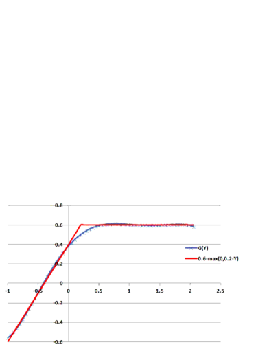
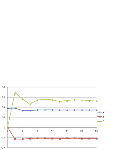
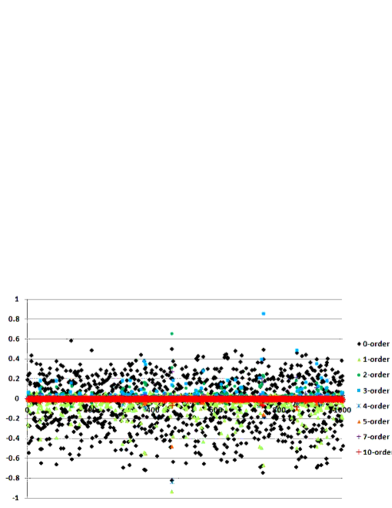
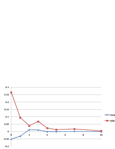
Figure 13: $T=1,\sigma=0.2,\alpha=0.4,\rho=-0.6,\kappa=0.1,c_{0}=0.01$, $c_{1}=0.4,\gamma=1,g_{1}=0.6$. $G(y)$ is a $5$-th order polynomial approximating $[0.6-\max(0,0.2-y)]$.

	$n=0$	$n=1$	$n=2$	$n=3$	$n=4$	$n=5$	$n=7$	$n=10$
mean	-0.052	-0.031	0.012	0.011	$-9.2\times 10^{-4}$	$-9.9\times 10^{-4}$	$1.4\times 10^{-3}$	$-9.0\times 10^{-4}$
stdev	0.27	0.095	0.040	0.069	0.024	0.013	0.017	$5.2\times 10^{-3}$

Table 6: Mean and standard deviation of $[\gamma H_{T}-\widetilde{V}^{(n)}_{T}]$ for the setup in Figure 13.

6 Conclusions

In this paper, a polynomial scheme of asymptotic expansion for BSDEs is proposed. We have shown that the polynomial expansion is uniquely determined by the recursive system of linear ODEs, which can be easily solved one-by-one by following the appropriate order of evaluation. We have studied possible applications to the pricing of European contingent claims as well as the exponential-utility optimization with terminal liability, each of which is provided several illustrative numerical examples.

A rigorous mathematical justification and more intensive numerical studies with realistic models are left for the future works. For example, a class of multi-factor Heston model proposed by Col et al. (2013) [8] has a nice structure of dependence to which the current scheme can be applied. Studying the BSDEs associated with the control problem with defaultable securities, such as those give by Pham (2010) [30], looks interesting, too.

Appendix A Proof of Lemma 2

We proceed as in the Heston’s model. Based on the dynamics (4.5) and (4.6), the forward dynamics of the hypothesized polynomial solution is given by

$$dV_{t}^{[n]}=\sum_{m=0}^{n}\sum_{k=0}^{m}\frac{X_{t}^{m-k}Y_{t}^{k}}{(m-k)!k!}\left\{\frac{\bigl{.}}{\bigr{.}}\dot{v}^{[n]}_{m-k,k}(t)\right.$$

$$\quad+\mathbb{I}_{(2\leq k)}k(k-1)\left(\frac{\sigma_{t}^{2}}{2}v^{[n]}_{m-k+2,k-2}(t)+\rho_{t}\sigma_{t}\alpha_{t}v^{[n]}_{m-k+1,k-1}(t)+\frac{\alpha_{t}^{2}}{2}v^{[n]}_{m-k,k}(t)\right)$$

$$\quad+\mathbb{I}_{(m\leq n-1,1\leq k)}k\Bigl{(}\sigma_{t}^{2}v^{[n]}_{m-k+2,k-1}(t)+2\rho_{t}\sigma_{t}\alpha_{t}v^{[n]}_{m-k+1,k}(t)+\alpha_{t}^{2}v^{[n]}_{m-k,k+1}(t)\Bigr{)}$$

$$\quad\left.+\mathbb{I}_{(m\leq n-2)}\left(\frac{\sigma_{t}^{2}}{2}v^{[n]}_{m-k+2,k}(t)+\rho_{t}\sigma_{t}\alpha_{t}v^{[n]}_{m-k+1,k+1}(t)+\frac{\alpha_{t}^{2}}{2}v^{[n]}_{m-k,k+2}(t)\right)\frac{\bigl{.}}{\bigr{.}}\right\}dt$$

$$\quad+\sum_{m=1}^{n}\sum_{k=0}^{m-1}v^{[n]}_{m-k,k}(t)\frac{X_{t}^{m-k-1}Y_{t}^{k}}{(m-k-1)!k!}dX_{t}$$

$$\quad+\sum_{m=1}^{n}\sum_{k=1}^{m}v^{[n]}_{m-k,k}(t)\frac{X_{t}^{m-k}Y_{t}^{k-1}}{(m-k)!(k-1)!}dY_{t}$$ (A.1)

which implies the control variables given in (4.14) and (4.14).

On the other hand, the $n$-th order part of the BSDE (4.9) is

$$V_{t}^{[n]}=\frac{X_{T}^{n}}{n!}\partial_{x}^{n}H(0)-\int_{t}^{T}Z_{s}^{[n]}dX_{s}-\int_{t}^{T}\Gamma_{s}^{[n]}dY_{s}$$

$$\quad-\int_{t}^{T}\left\{\frac{\beta}{2}\sigma(s)^{2}\left(\sum_{l=0}^{n-1}\frac{\partial_{x}^{l}b(0)}{l!}X_{s}^{l}Z_{s}^{[n-l]}+2\sum_{l=0}^{n-2}\frac{\partial_{x}^{l}b(0)}{l!}X_{s}^{l}Y_{s}Z_{s}^{[n-l-1]}\right.\right.$$

$$\qquad\left.\left.+\sum_{l=0}^{n-3}\frac{\partial_{x}^{l}b(0)}{l!}X_{s}^{l}Y_{s}^{2}Z_{s}^{[n-l-3]}\right)+\kappa_{s}Y_{s}\Gamma_{s}^{[n-1]}\right\}ds$$ (A.2)

Substituting the control variables by those in (4.14) and (4.14), one obtains

$$V_{t}^{[n]}=\frac{X_{T}^{n}}{n!}\partial_{x}^{n}H(0)-\int_{t}^{T}Z_{s}^{[n]}dX_{s}-\int_{t}^{T}\Gamma_{s}^{[n]}dY_{s}-\sum_{m=0}^{n}\sum_{k=0}^{m}\int_{t}^{T}\frac{X_{s}^{m-k}Y_{s}^{k}}{(m-k)!k!}$$

$$\times\left\{\mathbb{I}_{(m\leq n-1,1\leq k)}k\kappa_{s}v^{[n-1]}_{m-k,k}(s)+\mathbb{I}_{(m\leq n-1)}\frac{\beta}{2}\sigma_{s}^{2}\sum_{l=0}^{m-k}C_{(m-k,l)}\partial^{l}_{x}b(0)\right.$$

$$\quad\left.\times\left(v^{[n-l]}_{m-k-l+1,k}(s)+\mathbb{I}_{(1\leq k)}2k~{}v^{[n-l-1]}_{m-k-l+1,k-1}(s)+\mathbb{I}_{(2\leq k)}k(k-1)v^{[n-l-2]}_{m-k-l+1,k-2}(s)\right)\frac{\bigl{.}}{\bigr{.}}\right\}ds~{}.$$

By comparing the coefficients in the drift term, one obtains the linear ODEs as (4.15). If the forward SDE (A.1) is well-defined with the solution of (4.15), then it is clear that it gives one solution for the BSDE (A.2). The uniqueness of the polynomial solution is clear due to the linearity of the ODEs.

Appendix B Proof of Lemma 3

The dynamics of (5.9) and (5.10) gives the forward SDEs of the assumed polynomial (5.16) as

$$dV_{t}^{[n]}=\sum_{m=0}^{n}\sum_{k=0}^{m}\frac{X_{t}^{m-k}Y_{t}^{k}}{(m-k)!k!}\left\{\dot{v}^{[n]}_{m-k,k}(t)\frac{\bigl{.}}{\bigr{.}}\right.$$

$$\quad+\mathbb{I}_{(m\leq n-1,1\leq k)}k\left(\frac{\sigma_{t}^{2}}{2}v^{[n]}_{m-k+2,k-1}(t)+\rho_{t}\sigma_{t}\alpha_{t}v^{[n]}_{m-k+1,k}(t)+\frac{\alpha_{t}^{2}}{2}v^{[n]}_{m-k,k+1}(t)\right)$$

$$\quad\left.+\mathbb{I}_{(m\leq n-2)}\left(\frac{\sigma_{t}^{2}}{2}v^{[n]}_{m-k+2,k}(t)+\rho_{t}\sigma_{t}\alpha_{t}v^{[n]}_{m-k+1,k+1}(t)+\frac{\alpha_{t}^{2}}{2}v^{[n]}_{m-k,k+2}(t)\right)\frac{\bigl{.}}{\bigr{.}}\right\}dt$$

$$\quad+\sum_{m=1}^{n}\sum_{k=0}^{m-1}v^{[n]}_{m-k,k}(t)\frac{X_{t}^{m-k-1}Y_{t}^{k}}{(m-k-1)!k!}dX_{t}$$

$$\quad+\sum_{m=1}^{n}\sum_{k=1}^{m}v^{[n]}_{m-k,k}(t)\frac{X_{t}^{m-k}Y_{t}^{k-1}}{(m-k)!(k-1)!}dY_{t}$$ (B.1)

which then implies the control variables as in (5.17) and (5.18). On the other hand, the $n$-order BSDE of (5.13) is

$$V_{t}^{[n]}=\sum_{k=0}^{n}\frac{X_{T}^{n-k}Y_{T}^{k}}{(n-k)!k!}\gamma\partial_{x}^{n-k}\partial_{y}^{k}H(0,0)-\int_{t}^{T}Z_{s}^{[n]}dX_{s}-\int_{t}^{T}\Gamma_{s}^{[n]}dY_{s}$$

$$-\int_{t}^{T}\left\{\sum_{k=0}^{n}\frac{X_{s}^{n-k}Y_{s}^{k}}{(n-k)!k!}\frac{1}{2}\partial_{x}^{n-k}\partial_{y}^{k}\Theta(s,0,0)+\kappa_{s}Y_{s}\Gamma_{s}^{[n-1]}\right.$$

$$\qquad-\frac{\alpha(s)^{2}}{2}(1-\rho(s)^{2})\left(\sum_{l=1}^{n-1}\Gamma_{s}^{[l]}\Gamma_{s}^{[n-l]}+Y_{s}\sum_{l=1}^{n-2}\Gamma_{s}^{[l]}\Gamma_{s}^{[n-l-1]}\right)$$

$$\qquad\left.+\frac{\sigma(s)^{2}}{2}\Bigl{(}Z_{s}^{[n]}+Y_{s}Z_{s}^{[n-1]}\Bigr{)}\frac{\bigl{.}}{\bigr{.}}\right\}ds~{}.$$ (B.2)

Substituting (5.17) and (5.18) into the above expression and reordering the summation yield

$$V_{t}^{[n]}=\sum_{k=0}^{n}\frac{X_{T}^{n-k}Y_{T}^{k}}{(n-k)!k!}\gamma\partial_{x}^{n-k}\partial_{y}^{k}H(0,0)-\int_{t}^{T}Z_{s}^{[n]}dX_{s}-\int_{t}^{T}\Gamma_{s}^{[n]}dY_{s}$$

$$-\sum_{m=0}^{n}\sum_{k=0}^{m}\int_{t}^{T}\frac{X_{s}^{m-k}Y_{s}^{k}}{(m-k)!k!}\left\{\mathbb{I}_{(m=n)}\frac{1}{2}\partial_{x}^{n-k}\partial_{y}^{k}\Theta(s,0,0)+\mathbb{I}_{(m\leq n-1)}\frac{\sigma_{s}^{2}}{2}v^{[n]}_{m-k+1,k}(s)\frac{\bigl{.}}{}\right.$$

$$\quad+\mathbb{I}_{(m\leq n-1,1\leq k)}k\Bigl{(}\frac{\sigma_{s}^{2}}{2}v^{[n-1]}_{m-k+1,k-1}(s)+\kappa_{s}v^{[n-1]}_{m-k,k}(s)\Bigr{)}$$

$$-\frac{\alpha_{s}^{2}}{2}\xi_{s}^{2}\mathbb{I}_{(m\leq n-2)}\sum_{l=1}^{n-1}\sum_{j=1\vee[l+2-n+m]}^{l\wedge[m+1]}\sum_{p=1\vee[j-m+k]}^{j\wedge[k+1]}C_{(m-k,j-p)}C_{(k,p-1)}v^{[l]}_{j-p,p}(s)v^{[n-l]}_{m-k-j+p,k-p+2}(s)$$

$$\left.-\frac{\alpha_{s}^{2}}{2}\xi_{s}^{2}\mathbb{I}_{(1\leq m\leq n-2,1\leq k)}\sum_{l=1}^{n-2}\sum_{j=1\vee[l+2-n+m]}^{l\wedge m}\sum_{p=1\vee[j-m+k]}^{j\wedge k}C_{(m-k,j-p)}C_{(k,p)}pv^{[l]}_{j-p,p}(s)v^{[n-l-1]}_{m-k-j+p,k-p+1}(s)\right\}ds$$

(B.3)

By comparing the drift terms of (B.1) and (B.3), one obtains the system of linear ODEs as in Lemma 3. It is clear that if the forward SDE (B.1) with the solution of the ODEs is well-defined, it at least gives one solution for the BSDE of the $n$-th order (B.2). Due to the linearity of the ODEs, the solution should be unique within the assumed polynomial form.

Appendix C An exact solution for (5.11)

Suppose that both of the $H(x,y)$ and $\Theta(t,x,y)$ are linear functions of $(x,y)$:

$$H(x,y)=h_{x}x+h_{y}y+h_{0}$$ (C.1)

$$\Theta(t,x,y)=\Theta_{x}(t)x+\Theta_{y}(t)y+\Theta_{0}(t)$$ (C.2)

where $(h_{x},h_{y},h_{0})$ are constants and $(\Theta_{x}(t),\Theta_{y}(t),\Theta_{0}(t))_{t}$ are some deterministic functions of time. Then, it is almost immediate to notice that a linear value function and the deterministic control variables can provide an exact solution:

$$V_{t}=v_{x}(t)X_{t}+v_{y}(t)Y_{t}+v_{0}(t)$$ (C.3)

$$Z_{t}=v_{x}(t)$$ (C.4)

$$\Gamma_{t}=v_{y}(t)$$ (C.5)

where $(v_{x}(t),v_{y}(t),v_{0}(t))$ are deterministic functions of time.

The ODEs which fixes $v_{x},v_{y},v_{0}$ can be obtained quite similarly to the discussed approximation scheme. On the one hand, the dynamics of the proposed solution becomes

$$dV_{t} = \Bigl{(}\dot{v}_{x}(t)X_{t}+\dot{v}_{y}(t)Y_{t}+\dot{v}_{0}(t)\Bigr{)}dt$$ (C.6)

$$+v_{x}(t)dX_{t}+v_{y}(t)dY_{t}~{}.$$

On the other hand, by inserting the assumed form of control variables to (5.11), one obtains

$$V_{t}=\gamma\Bigl{[}h_{x}X_{T}+h_{y}Y_{T}+h_{0}\Bigr{]}-\int_{t}^{T}v_{x}(s)dX_{s}-\int_{t}^{T}v_{y}(s)dY_{s}$$

$$\quad-\int_{t}^{T}\left\{\frac{1}{2}\Bigl{(}\Theta_{x}(s)X_{s}+\Theta_{y}(s)Y_{s}+\Theta_{0}(s)\Bigr{)}+\kappa(s)v_{y}(s)Y_{s}\right.$$ (C.7)

$$\qquad\left.+\frac{1}{2}\Bigl{(}\sigma(s)^{2}v_{x}(s)-\alpha(s)^{2}(1-\rho(s)^{2})v_{y}(s)^{2}\Bigr{)}(1+Y_{s})\right\}ds~{}.$$ (C.8)

Thus, the the system of ODEs including a Riccati-type for $v_{y}$

$$\dot{v}_{x}(t)=\frac{1}{2}\Theta_{x}(t)$$ (C.9)

$$\dot{v}_{y}(t)=\frac{1}{2}\Bigl{(}\sigma(t)^{2}v_{x}(t)-\alpha(t)^{2}(1-\rho(s)^{2})v_{y}(t)^{2}\Bigr{)}+\kappa(t)v_{y}(t)+\frac{1}{2}\Theta_{y}(t)$$ (C.10)

$$\dot{v}_{0}(t)=\frac{1}{2}\Bigl{(}\sigma(t)^{2}v_{x}(t)-\alpha(t)^{2}(1-\rho(s)^{2})v_{y}(t)^{2}\Bigr{)}+\frac{1}{2}\Theta_{0}(t)$$ (C.11)

with the terminal conditions

$$v_{x}(T)=\gamma h_{x},\quad v_{y}(T)=\gamma h_{y},\quad v_{0}(T)=\gamma h_{0}$$ (C.12)

gives an exact solution if $v_{y}$ (and hence the others) has a finite solution for the relevant time interval $t\in[0,T]$.

References

- [1] Bender, C. and Denk, R., 2007, “A forward scheme for backward SDEs,” Stochastic Processes and their Applications, 117,12, 1793-1823.
- [2] Bismut, J.M., 1973, “Conjugate Convex Functions in Optimal Stochastic Control,” J. Math. Anal. Apl. 44, 384-404.
- [3] Bianchetti, M. and Morini, M. (editors), 2013, “Interest Rate Models after the Financial Crisis,” Risk books, UK.
- [4] Blinnikov, S. and Moessner, R., 1998, “Expansions for nearly Gaussian distributions,” Astron. Astrophys. Suppl. Ser., Vol. 130, 1, 193-205.
- [5] Brigo, D., Morini, M. and Pallavicini, A., 2013, “Counterparty, Credit Risk, Collateral and Funding,” Wiley, UK.
- [6] Bouchard, B. and Touzi, N., 2004, “Discrete-time approximation and Monte-Carlo simulation of backward stochastic differential equations,” Stochastic Processes and their Applications, 111, 2, 175-206.
- [7] Carmona, R (editor), 2009, “Indifference Pricing,” Princeton University Press, UK.
- [8] Col, A.D., Gnoatto, A. and Grasselli, M., 2013, “Smiles all around: FX joint calibration in a multi-Heston model,” Journal of Banking and Finance, Vol. 37, 10, 3799-3818.
- [9] Crépey, S., 2013, “Bilateral Counterparty Risk under Funding Constraints-Part I:Pricing, Part II: CVA,” to appear in Mathematical Finance.
- [10] Crépey, S., 2013, “Financial Modeling: A Backward Stochastic Differential Equations Perspective,” Springer, UK.
- [11] Cvitanić, J. and Zhang, J., 2013, “Contract Theory in Continuous-Time Methods,” Springer, Berlin.
- [12] Delong, L., 2013, “Backward Stochastic Differential Equations with Jumps and their Actuarial and Financial Applications,” Springer, UK.
- [13] Douglas, J., Ma, J. and Protter, P., 1996, “Numerical Methods for Forward-Backward Stochastic Differential Equations,” The Annals of Applied Probability, 6, 940-968.
- [14] Duffie, D. and Huang, M., 1996, “Swap Rates and Credit Quality,” Journal of Finance, Vol. 51, No. 3, 921.
- [15] El Karoui, N. and Mazliak, L (editors), 1997, “Backward stochastic differential equations,” Longman, US.
- [16] Fujii, M. and Takahashi, A., 2013, “Derivative Pricing under Asymmetric and Imperfect Collateralization and CVA, h Quantitative Finance, Vol. 13, Issue 5, 749-768.
- [17] Fujii, M. and Takahashi, A., 2012a, “Perturbative Expansion Technique for Non-Linear FBSDEs with Interacting Particle Method,” CARF-working paper series, available at arXiv and SSRN.
- [18] Fujii, M. and Takahashi, A., 2012b, “Analytical Approximation for Non-Linear FBSDEs with Perturbation Scheme, ” International Journal of Theoretical and Applied Finance, 15, 1250034 (24).
- [19] Fujii, M. and Takahashi, A., 2013, “Making mean-variance hedging implementable in a partially observable market,” Quantitative Finance, DOI: 10.1080/14697688.2013.867453
- [20] Fujii, M. and Takahashi, A., 2014, “Optimal Hedging for Fund & Insurance Managers with Partially Observable Investment Flows,” Forthcoming in Quantitative Finance.
- [21] Gobet, E. and Lemor, J.-P. and Warin, X., 2005, “A regression-based Monte Carlo method to solve backward stochastic differential equations,” The Annals of Applied Probability, 15, 3, 2172-2202.
- [22] Gobet, E. and Labart, C., 2010, “Solving BSDE with Adaptive Control Variate,” SIAM Journal on Numerical Analysis, 48, 257-277.
- [23] Henry-Labordere, P., 2012, “Cutting CVA’s Complexity,” Risk magazine, Jul issue.
- [24] Kunitomo, N. and Takahashi, A., 2003, “On validity of the Asymptotic Expansion Approach in Contingent Claim Analysis,” The Annals of Applied Probability, 13, no. 3, 914-952.
- [25] Ma, J. and Yong, J., 2000 “Forward-Backward Stochastic Differential Equations and their Applications,” Springer, Berlin.
- [26] Ma, J., Protter, P., and Yong, J., 1994, “Solving forward-backward stochastic differential equations explicitly,” Prob & Related Fields, 98, 339-359.
- [27] Mania, M. and Tevzadze, R., 2003, “Backward Stochastic PDE and Imperfect Hedging,” International Journal of Theoretical and Applied Finance, Vol. 6, 7, 663-692.
- [28] Mania, M. and Tevzadze, R., 2008, “Backward Stochastic Partial Differential Equations Related to Utility Maximization and Hedging, ” Journal of Mathematical Science, Vol. 153, 3, 291-380.
- [29] Pardoux, E., and Peng, S., 1990, “Adapted Solution of a Backward Stochastic Differential Equations,” Systems Control Lett., 14, 55-61.
- [30] Pham, H., 2010, “Stochastic control under progressive enlargement of filtrations and applications to multiple defaults risk management,” Stochastic Processes and their Applications, 120, 1795-1820.
- [31] Schroder, M. and Skiadas, C., 1999, “Optimal Consumption and Portfolio Selection with Stochastic Differential Utility,” Journal of Economic Theory, 89, 68-126.
- [32] Takahashi, A., 1999, “An Asymptotic Expansion Approach to Pricing Contingent Claims,” Asia-Pacific Financial Markets, 6, 115-151.
- [33] Takahashi, A. and Yamada, T., 2013, “On an Asymptotic Expansion of Forward-Backward SDEs with a Perturbation Driver,” CARF working paper series. CARF-F-326.
- [34] Watanabe, S., 1987, “Analysis of Wiener functionals (Malliavin calculus) and its applications to heat kernels, ” Annals of Probability, 15, 1-39.
- [35] Yoshida, N., 1992a, “Asymptotic Expansion for Statistics Related to Small Diffusions,” J. Japan Statist. Soc., Vol. 22, No. 2, 139-159.
- [36] Yoshida, N., 1992b, “Asymptotic Expansions of Maximum Likelihood Estimators for Small Diffusions via the Theory of Malliavin-Watanabe,” Probability Theory and Related Fields, 92, 275-311.
- [37] Zariphopoulou, T., 2001, “A solution approach to valuation with unhedgeable risks,” Finance and Stochastics, 5, 61-82.