Spin injection from a ferromagnet into a semiconductor in the case of a rough interface

Abstract

The effect of the interface roughness on the spin injection from a ferromagnet into a semiconductor is studied theoretically. Even a small interface irregularity can lead to a significant enhancement of the injection efficiency. When a typical size of the irregularity, $a$, is within a domain $\lambda_{\scriptscriptstyle F}\ll a\ll\lambda_{\scriptscriptstyle N}$, where $\lambda_{\scriptscriptstyle F}$ and $\lambda_{\scriptscriptstyle N}$ are the spin-diffusion lengths in the ferromagnet and semiconductor, respectively, the geometrical enhancement factor is $\sim\lambda_{\scriptscriptstyle N}/a$. The origin of the enhancement is the modification of the local electric field on small scales $\sim a$ near the interface. We demonstrate the effect of enhancement by considering a number of analytically solvable examples of injection through curved ferromagnet-semiconductor interfaces. For a generic curved interface the enhancement factor is $\sim\lambda_{\scriptscriptstyle N}/R$, where $R$ is the local radius of curvature.

I Introduction

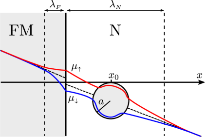
Figure 1: (Color online) Illustration of the spin injection through a planar interface, Ref. wyder, , in the presence of a ferromagnetic cylinder with a small radius $a\ll\lambda_{\scriptscriptstyle N}$ located at distance, $x_{0}$, such that $a\ll x_{0}\ll\lambda_{\scriptscriptstyle N}$ from the F/N interface. The behaviors of the chemical potentials for up and down spins is shown schematically.

In a seminal paper Ref. wyder, the efficiency of spin injection from a ferromagnet into a normal metal was quantified. In the minimal model considered in Ref. wyder, spin injection resulted from the behavior of four functions $\mu^{\scriptscriptstyle F}_{\scriptscriptstyle\uparrow}(x),\mu^{\scriptscriptstyle F}_{\scriptscriptstyle\downarrow}(x),\mu^{\scriptscriptstyle N}_{\scriptscriptstyle\uparrow}(x)$ and $\mu^{\scriptscriptstyle N}_{\scriptscriptstyle\downarrow}(x)$, which are the chemical potentials for the spin-up and spin-down electrons near the boundary. In the ferromagnetic region, $x<0$, and in the metallic region, $x>0$, see Fig. 1, the functions $\mu_{\scriptscriptstyle\uparrow}$ and $\mu_{\scriptscriptstyle\uparrow}$ are related by the diffusion equations

$$\frac{d^{2}}{dx^{2}}\left(\mu^{\scriptscriptstyle F}_{\scriptscriptstyle\uparrow}-\mu^{\scriptscriptstyle F}_{\scriptscriptstyle\downarrow}\right)=\frac{\mu^{\scriptscriptstyle F}_{\scriptscriptstyle\uparrow}-\mu^{\scriptscriptstyle F}_{\scriptscriptstyle\downarrow}}{\lambda_{\scriptscriptstyle F}^{2}},\frac{d^{2}}{dx^{2}}\left(\mu^{\scriptscriptstyle N}_{\scriptscriptstyle\uparrow}-\mu^{\scriptscriptstyle N}_{\scriptscriptstyle\downarrow}\right)=\frac{\mu^{\scriptscriptstyle N}_{\scriptscriptstyle\uparrow}-\mu^{\scriptscriptstyle N}_{\scriptscriptstyle\downarrow}}{\lambda_{\scriptscriptstyle N}^{2}},$$ (1)

where $\lambda_{\scriptscriptstyle F}$ and $\lambda_{\scriptscriptstyle N}$ are the spin diffusion lengths in the ferromagnet and normal metal, respectively. The system Eq. (1) should be supplemented by the boundary conditions

$$\left.{j}^{\scriptscriptstyle F}_{\scriptscriptstyle\uparrow}=\sigma^{\scriptscriptstyle F}_{\scriptscriptstyle\uparrow}\frac{\partial\mu^{\scriptscriptstyle F}_{\scriptscriptstyle\uparrow}}{\partial x}\right|_{x=0^{-}} =\left.j^{\scriptscriptstyle N}_{\scriptscriptstyle\uparrow}=\sigma^{\scriptscriptstyle N}\frac{\partial\mu^{\scriptscriptstyle N}_{\scriptscriptstyle\uparrow}}{\partial x}\right|_{x=0^{+}},$$

$$\left.{j}^{\scriptscriptstyle F}_{\scriptscriptstyle\downarrow}=\sigma^{\scriptscriptstyle F}_{\scriptscriptstyle\downarrow}\frac{\partial\mu^{\scriptscriptstyle F}_{\scriptscriptstyle\downarrow}}{\partial x}\right|_{x=0^{-}} =\left.{j}^{\scriptscriptstyle N}_{\scriptscriptstyle\downarrow}=\sigma^{\scriptscriptstyle N}\frac{\partial\mu^{\scriptscriptstyle N}_{\scriptscriptstyle\downarrow}}{\partial x}\right|_{x=0^{+}},$$ (2)

which expresses the continuity of the components of the current densities, $j_{\scriptscriptstyle\uparrow}$ and $j_{\scriptscriptstyle\downarrow}$, normal to the interface. Here $\sigma^{\scriptscriptstyle F}_{\scriptscriptstyle\uparrow}$ and $\sigma^{\scriptscriptstyle F}_{\scriptscriptstyle\downarrow}$ are the conductivities of up-spins and down-spins in the ferromagnetic region, while $\sigma^{\scriptscriptstyle N}$ is the (spin independent) conductivity in the metallic region. Another boundary condition, which follows from the continuity of $\mu_{\scriptscriptstyle\uparrow}$ and $\mu_{\scriptscriptstyle\downarrow}$ at the boundary $x=0$ reads

$$\left.\mu^{\scriptscriptstyle F}_{\scriptscriptstyle\uparrow}-\mu^{\scriptscriptstyle F}_{\scriptscriptstyle\downarrow}\right|_{x=0^{-}}=\left.\mu^{\scriptscriptstyle N}_{\scriptscriptstyle\uparrow}-\mu^{\scriptscriptstyle N}_{\scriptscriptstyle\downarrow}\right|_{x=0^{+}}.$$ (3)

General solutions of Eq. (1), which decay away from the boundary, are the simple exponents

$$\mu^{\scriptscriptstyle F}_{\scriptscriptstyle\uparrow} =\mu_{0}^{\scriptscriptstyle F}(x)+A_{\scriptscriptstyle\uparrow}e^{x/\lambda_{\scriptscriptstyle F}}, \mu_{\scriptscriptstyle\uparrow}^{\scriptscriptstyle N} =\mu_{0}^{\scriptscriptstyle N}(x)+B_{\scriptscriptstyle\uparrow}e^{-x/\lambda_{\scriptscriptstyle N}},$$ (4)

$$\mu_{\scriptscriptstyle\downarrow}^{\scriptscriptstyle F} =\mu_{0}^{\scriptscriptstyle F}(x)+A_{\scriptscriptstyle\downarrow}e^{x/\lambda_{\scriptscriptstyle F}}, \mu_{\scriptscriptstyle\downarrow}^{\scriptscriptstyle N} =\mu_{0}^{\scriptscriptstyle N}(x)+B_{\scriptscriptstyle\downarrow}e^{-x/\lambda_{\scriptscriptstyle N}},$$ (5)

where $\mu_{0}^{\scriptscriptstyle F}(x)$ and $\mu_{0}^{\scriptscriptstyle N}(x)$ are the linear functions with slopes proportional to the net current, $j$; the ratio of the slopes is $(\sigma^{\scriptscriptstyle F}_{\scriptscriptstyle\uparrow}+\sigma^{\scriptscriptstyle F}_{\scriptscriptstyle\downarrow})/2\sigma^{\scriptscriptstyle N}$. The conditions Eqs. (2), (3) impose the following relations between the coefficients $A_{\scriptscriptstyle\uparrow},A_{\scriptscriptstyle\downarrow},B_{\scriptscriptstyle\uparrow}$, and $B_{\scriptscriptstyle\downarrow}$

$$\sigma^{\scriptscriptstyle F}_{\scriptscriptstyle\uparrow}\left(\frac{j}{\sigma^{\scriptscriptstyle F}_{\scriptscriptstyle\uparrow}+\sigma^{\scriptscriptstyle F}_{\scriptscriptstyle\downarrow}}+\frac{A_{\scriptscriptstyle\uparrow}}{\lambda_{\scriptscriptstyle F}}\right) =\sigma^{\scriptscriptstyle N}\left(\frac{j}{2\sigma^{\scriptscriptstyle N}}-\frac{B_{\scriptscriptstyle\uparrow}}{\lambda_{\scriptscriptstyle N}}\right)=j^{\scriptscriptstyle N}_{\scriptscriptstyle\uparrow},$$ (6)

$$\sigma^{\scriptscriptstyle F}_{\scriptscriptstyle\downarrow}\left(\frac{j}{\sigma^{\scriptscriptstyle F}_{\scriptscriptstyle\uparrow}+\sigma^{\scriptscriptstyle F}_{\scriptscriptstyle\downarrow}}+\frac{A_{\scriptscriptstyle\downarrow}}{\lambda_{\scriptscriptstyle F}}\right) =\sigma^{\scriptscriptstyle N}\left(\frac{j}{2\sigma^{\scriptscriptstyle N}}-\frac{B_{\scriptscriptstyle\downarrow}}{\lambda_{\scriptscriptstyle N}}\right)=j^{\scriptscriptstyle N}_{\scriptscriptstyle\downarrow},$$ (7)

$$A_{\scriptscriptstyle\uparrow}-A_{\scriptscriptstyle\downarrow} =B_{\scriptscriptstyle\uparrow}-B_{\scriptscriptstyle\downarrow}.$$ (8)

These relations together with total current conservation, $j^{\scriptscriptstyle N}_{\scriptscriptstyle\uparrow}+j^{\scriptscriptstyle N}_{\scriptscriptstyle\downarrow}=j$, are sufficient to find the degree of polarization of the injected currentwyder

$$\mathcal{P}=\frac{j^{\scriptscriptstyle N}_{\scriptscriptstyle\uparrow}-j^{\scriptscriptstyle N}_{\scriptscriptstyle\downarrow}}{j^{\scriptscriptstyle N}_{\scriptscriptstyle\uparrow}+j^{\scriptscriptstyle N}_{\scriptscriptstyle\downarrow}}=\dfrac{\sigma^{\scriptscriptstyle N}\left(\dfrac{1}{\sigma^{\scriptscriptstyle F}_{\scriptscriptstyle\downarrow}}-\dfrac{1}{\sigma^{\scriptscriptstyle F}_{\scriptscriptstyle\uparrow}}\right)\gamma}{2+\sigma^{\scriptscriptstyle N}\left(\dfrac{1}{\sigma^{\scriptscriptstyle F}_{\scriptscriptstyle\downarrow}}+\dfrac{1}{\sigma^{\scriptscriptstyle F}_{\scriptscriptstyle\uparrow}}\right)\gamma},$$ (9)

where the parameter $\gamma$ is defined as

$$\gamma=\frac{\lambda_{\scriptscriptstyle F}}{\lambda_{\scriptscriptstyle N}}.$$ (10)

It follows from Eq. (9) that the injection is efficient when the conductivities of the ferromagnet and the normal metal are of the same order. And indeed, in subsequent experimentsvanWeesCointoAlNonlocal ; MesoscopicIsland ; CrossedGeometry1DCalculation the injection was demonstrated for the contacts of ferromagnets with paramagnetic metals.

By the year 2000 it became apparent that applications of the spin-injection effect in the information technology require the injection from a ferromagnet into a semiconductor. Thus the subsequent experimental studies, see e.g. Refs. tip, ; InjectionIntoNanowire, ; vanWeesGrapheneInjection, ; LatestFertNonlocal, , were focused on achieving this goal. The detailed account of the results on spin-injection devices based on ferromagnet-silicon contacts can be found in a recent review Ref. reviewSi, .

It was first pointed out in Ref. molenkamp, that the large ratio of conductivities $\sigma^{\scriptscriptstyle F}/\sigma^{\scriptscriptstyle N}\sim 10^{4}$ constitutes a fundamental obstacle for the spin injection limiting it to $\sim 0.1$ percentmolenkamp . To circumvent this “conductivity mismatch” problem it was proposedrashba ; review to introduce a tunnel barrier between the ferromagnet and semiconductor. However Eq. (9) also suggests that the additional source of weakness of injection is the the smallness of the parameter $\gamma$, Eq. (10). While the spin diffusion length in the ferromagnet is typically $\lambda_{\scriptscriptstyle F}\sim 10$ nm, the length $\lambda_{\scriptscriptstyle N}$ is much larger. From the experiment on injection into InN nanowiresInjectionIntoNanowire the value $\lambda_{\scriptscriptstyle N}\sim 200$ nm was inferred. Even higher values of $\lambda_{\scriptscriptstyle N}$ between $5$ and $50$ $\mu$m have been reported for spin injection into GaAs wiresCrowell1 ; Crowell2 .

The main message of the present paper is that, with small value of $\gamma$, the polarization of the injected current can be strongly enhanced by the roughness of the ferromagnet-semiconductor interface with a spatial scale $\sim\lambda_{\scriptscriptstyle F}$. On the qualitative level, this enhancement is due to the local enhancement of electric field near a curved surface. Note that this effect could not be uncovered in the earlier theories of spin transportFertMultilayer ; GorkovDzeroMultilayer ; khaetskii ; 5layers ; Flatte ; German in multilayered structures, where it was implicit that the chemical potentials change along one dimension only.

In Sections II and III we will illustrate our message for some toy models which allow a rigorous analytical solution. In Sect. IV we will consider the enhancement of injection due to interface inhomogeneities for more realistic geometries. Sect. V concludes the paper.

II Ferromagnetic grain near the interface

Assume that a ferromagnetic cylinder of radius, $a$, is embedded into a semiconducting region at distance, $x_{0}$, from the interface. The distance $x_{0}$ is much bigger than $a$ but much smaller than the spin diffusion length $\lambda_{\scriptscriptstyle N}$, see Fig. 1. The presence of the cylinder modifies the current distribution in semiconductor. In principle, this modification depends on $\sigma_{\scriptscriptstyle\uparrow}^{\scriptscriptstyle F}$ and $\sigma_{\scriptscriptstyle\downarrow}^{\scriptscriptstyle F}$, but when both conductivities are bigger than $\sigma^{\scriptscriptstyle N}$, the correction to the current density depends only on the distance, ${\bm{\rho}}$, to the center of the cylinder

$${\bm{j}}^{\scriptscriptstyle N}({\bm{\rho}})={\bm{j}}^{\scriptscriptstyle 0}-{\bm{j}}^{\scriptscriptstyle 0}\frac{a^{2}}{\rho^{2}}+\frac{2a^{2}({\bm{j}}^{\scriptscriptstyle 0}\cdot{\bm{\rho}}){\bm{\rho}}}{\rho^{4}}.$$ (11)

This textbook result emerges from matching the tangent components of electric field and normal components of current at the surface of the cylinder. Our goal is to derive the relation similar to Eq. (11) for the spin current density

$${\bm{j}}_{s}={\bm{j}}_{\scriptscriptstyle\uparrow}-{\bm{j}}_{\scriptscriptstyle\downarrow}.$$ (12)

In the absence of the cylinder, this density is given by ${\bm{j}}_{s}=\mathcal{P}{\bm{j}}^{\scriptscriptstyle 0}\exp(-x/\lambda_{\scriptscriptstyle N})$, with $\mathcal{P}$ defined by Eq. (9). To achieve this goal, one has to find the functions $\mu_{\scriptscriptstyle\uparrow}^{\scriptscriptstyle N}$ and $\mu_{\scriptscriptstyle\downarrow}^{\scriptscriptstyle N}$ from the diffusion equation Eq. (1) and match them and the normal components of current with the corresponding solutions of the diffusion equation for $\mu_{\scriptscriptstyle\uparrow}^{\scriptscriptstyle F}$ and $\mu_{\scriptscriptstyle\downarrow}^{\scriptscriptstyle F}$ inside the cylinder.

For distances, $x_{0}$, in the domain $a\ll x_{0}\ll\lambda_{\scriptscriptstyle N}$ the solutions for $\mu^{\scriptscriptstyle N}_{\scriptscriptstyle\uparrow}$ and $\mu^{\scriptscriptstyle N}_{\scriptscriptstyle\downarrow}$ still have the “dipole” form

$$\mu_{\scriptscriptstyle\uparrow}^{\scriptscriptstyle N} =\alpha_{\scriptscriptstyle\uparrow}+\beta_{\scriptscriptstyle\uparrow}\rho\cos\theta+\frac{F}{\rho}\cos\theta,$$ (13)

$$\mu_{\scriptscriptstyle\downarrow}^{\scriptscriptstyle N} =\alpha_{\scriptscriptstyle\downarrow}+\beta_{\scriptscriptstyle\downarrow}\rho\cos\theta+\frac{G}{\rho}\cos\theta.$$ (14)

Here, the constants $\alpha_{\scriptscriptstyle\uparrow}$, $\alpha_{\scriptscriptstyle\downarrow}$ are the values of $\mu_{\scriptscriptstyle\uparrow}^{\scriptscriptstyle N}$ and $\mu_{\scriptscriptstyle\downarrow}^{\scriptscriptstyle N}$ at $x=0$. Similarly, $\beta_{\scriptscriptstyle\uparrow}$ and $\beta_{\scriptscriptstyle\downarrow}$ are $\frac{d\mu^{\scriptscriptstyle N}_{\scriptscriptstyle\uparrow}}{dx}$ and $\frac{d\mu^{\scriptscriptstyle N}_{\scriptscriptstyle\downarrow}}{dx}$ at $x=0$, which can be cast in the form

$$\beta_{\scriptscriptstyle\uparrow(\downarrow)}=\frac{j^{0}}{2\sigma^{\scriptscriptstyle N}}\left(1\pm\mathcal{P}\right).$$ (15)

With the same accuracy as Eq. (11), this specification of $\beta_{\scriptscriptstyle\uparrow}$ and $\beta_{\scriptscriptstyle\downarrow}$ is valid when $x_{0}\gg a$, i.e. when the feedback of the cylinder on $\mu^{\scriptscriptstyle N}_{\scriptscriptstyle\uparrow}$ and $\mu^{\scriptscriptstyle N}_{\scriptscriptstyle\downarrow}$ near the boundary is negligible.

With regard to the net current distribution, the current density is constant inside the cylinder. This is, however, not the case for the spin density distribution, where $\mu_{\scriptscriptstyle\uparrow}$ and $\mu_{\scriptscriptstyle\downarrow}$ should be found from the diffusion equation, Eq. (1). It appears that in cylindrical coordinates we can, similarly to Eq. (11), keep only the solutions corresponding to the zeroth and the first angular momenta

$$\mu_{\scriptscriptstyle\uparrow}^{\scriptscriptstyle F}-\mu_{\scriptscriptstyle\downarrow}^{\scriptscriptstyle F}=AI_{0}\left(\frac{\rho}{\lambda_{\scriptscriptstyle F}}\right)+BI_{1}\left(\frac{\rho}{\lambda_{\scriptscriptstyle F}}\right)\cos\theta,$$ (16)

where $I_{0}(z)$ and $I_{1}(z)$ are the modified Bessel functions. Eq. (16) describes the decay of spin imbalance upon approaching the center of the cylinder. On the other hand, it follows from the local current conservation,       $\nabla\cdot({\bm{j}}_{\scriptscriptstyle\uparrow}+{\bm{j}}_{\scriptscriptstyle\downarrow})=0$, that the combination of $\sigma^{\scriptscriptstyle F}_{\scriptscriptstyle\uparrow}\mu^{\scriptscriptstyle F}_{\scriptscriptstyle\uparrow}+\sigma^{\scriptscriptstyle F}_{\scriptscriptstyle\downarrow}\mu^{\scriptscriptstyle F}_{\scriptscriptstyle\downarrow}$ does not decay, i.e.

$$\sigma^{\scriptscriptstyle F}_{\scriptscriptstyle\uparrow}\mu^{\scriptscriptstyle F}_{\scriptscriptstyle\uparrow}+\sigma^{\scriptscriptstyle F}_{\scriptscriptstyle\downarrow}\mu^{\scriptscriptstyle F}_{\scriptscriptstyle\downarrow}=(\sigma^{\scriptscriptstyle F}_{\scriptscriptstyle\uparrow}+\sigma^{\scriptscriptstyle F}_{\scriptscriptstyle\downarrow})C+D\rho\cos\theta.$$ (17)

The constants $C$, $D$ together with the constants $A$ and $B$ should be found from the boundary conditions at $\rho=a$. Matching $\mu^{\scriptscriptstyle N}_{\scriptscriptstyle\uparrow}$ and $\mu^{\scriptscriptstyle F}_{\scriptscriptstyle\uparrow}$ at $\rho=a$ yields

$$C+\frac{\sigma^{\scriptscriptstyle F}_{\scriptscriptstyle\downarrow}}{\sigma^{\scriptscriptstyle F}_{\scriptscriptstyle\uparrow}+\sigma^{\scriptscriptstyle F}_{\scriptscriptstyle\downarrow}}AI_{0}\left(\frac{a}{\lambda_{\scriptscriptstyle F}}\right) =\alpha_{\scriptscriptstyle\uparrow},$$ (18)

$$\frac{Da}{\sigma^{\scriptscriptstyle F}_{\scriptscriptstyle\uparrow}+\sigma^{\scriptscriptstyle F}_{\scriptscriptstyle\downarrow}}+\frac{\sigma^{\scriptscriptstyle F}_{\scriptscriptstyle\downarrow}B}{\sigma^{\scriptscriptstyle F}_{\scriptscriptstyle\uparrow}+\sigma^{\scriptscriptstyle F}_{\scriptscriptstyle\downarrow}}I_{1}\left(\frac{a}{\lambda_{\scriptscriptstyle F}}\right) =\beta_{\scriptscriptstyle\uparrow}a+\frac{F}{a}.$$ (19)

Similar equations originate from matching $\mu^{\scriptscriptstyle N}_{\scriptscriptstyle\downarrow}$ and $\mu^{\scriptscriptstyle F}_{\scriptscriptstyle\downarrow}$.

The condition, $\left.\sigma^{\scriptscriptstyle F}_{\scriptscriptstyle\uparrow}\frac{\partial\mu^{\scriptscriptstyle F}_{\scriptscriptstyle\uparrow}}{\partial\rho}\right|_{\rho=a}\!=\!\left.\sigma^{\scriptscriptstyle N}\frac{\partial\mu^{\scriptscriptstyle N}_{\scriptscriptstyle\uparrow}}{\partial\rho}\right|_{\rho=a}$, of the continuity of the radial current results in

$$\frac{\sigma^{\scriptscriptstyle F}_{\scriptscriptstyle\uparrow}\sigma^{\scriptscriptstyle F}_{\scriptscriptstyle\downarrow}}{\sigma^{\scriptscriptstyle F}_{\scriptscriptstyle\uparrow}+\sigma^{\scriptscriptstyle F}_{\scriptscriptstyle\downarrow}}\frac{A}{\lambda_{\scriptscriptstyle F}}I_{0}^{\prime}\left(\frac{a}{\lambda_{\scriptscriptstyle F}}\right) =0,$$ (20)

$$\frac{\sigma^{\scriptscriptstyle F}_{\scriptscriptstyle\uparrow}D}{\sigma^{\scriptscriptstyle F}_{\scriptscriptstyle\uparrow}+\sigma^{\scriptscriptstyle F}_{\scriptscriptstyle\downarrow}}+\frac{\sigma^{\scriptscriptstyle F}_{\scriptscriptstyle\uparrow}\sigma^{\scriptscriptstyle F}_{\scriptscriptstyle\downarrow}}{\sigma^{\scriptscriptstyle F}_{\scriptscriptstyle\uparrow}+\sigma^{\scriptscriptstyle F}_{\scriptscriptstyle\downarrow}}\frac{B}{\lambda_{\scriptscriptstyle F}}I_{1}^{\prime}\left(\frac{a}{\lambda_{\scriptscriptstyle F}}\right) =\sigma^{\scriptscriptstyle N}\left(\beta_{\scriptscriptstyle\uparrow}-\frac{F}{a^{2}}\right).$$ (21)

Eqs. (19), (21) express the continuity of the $\cos\theta$ terms in $\mu_{\scriptscriptstyle\uparrow}$ and ${\bm{j}}_{\scriptscriptstyle\uparrow}$. The corresponding conditions for $\mu_{\scriptscriptstyle\downarrow}$ and ${\bm{j}}_{\scriptscriptstyle\downarrow}$ read

$$\frac{Da}{\sigma^{\scriptscriptstyle F}_{\scriptscriptstyle\uparrow}+\sigma^{\scriptscriptstyle F}_{\scriptscriptstyle\downarrow}}-\frac{\sigma^{\scriptscriptstyle F}_{\scriptscriptstyle\uparrow}B}{\sigma^{\scriptscriptstyle F}_{\scriptscriptstyle\uparrow}+\sigma^{\scriptscriptstyle F}_{\scriptscriptstyle\downarrow}}I_{1}\left(\frac{a}{\lambda_{\scriptscriptstyle F}}\right) =\beta_{\scriptscriptstyle\downarrow}a+\frac{G}{a},$$ (22)

$$\frac{\sigma^{\scriptscriptstyle F}_{\scriptscriptstyle\downarrow}D}{\sigma^{\scriptscriptstyle F}_{\scriptscriptstyle\uparrow}+\sigma^{\scriptscriptstyle F}_{\scriptscriptstyle\downarrow}}-\frac{\sigma^{\scriptscriptstyle F}_{\scriptscriptstyle\uparrow}\sigma^{\scriptscriptstyle F}_{\scriptscriptstyle\downarrow}}{\sigma^{\scriptscriptstyle F}_{\scriptscriptstyle\uparrow}+\sigma^{\scriptscriptstyle F}_{\scriptscriptstyle\downarrow}}\frac{B}{\lambda_{\scriptscriptstyle F}}I_{1}^{\prime}\left(\frac{a}{\lambda_{\scriptscriptstyle F}}\right) =\sigma^{\scriptscriptstyle N}\left(\beta_{\scriptscriptstyle\downarrow}-\frac{G}{a^{2}}\right).$$ (23)

Note now, that the four conditions Eqs. (19), (21), (22), and (23) form a closed system of equations for the variables $D,B,F,$ and $G$. Note also, that it is these four variables which are responsible for the spin current. Solving this system yields

$${\bm{j}}^{\scriptscriptstyle N}_{s}({\bm{\rho}})={\bm{j}}^{\scriptscriptstyle 0}_{s}-\left(a^{2}\frac{\mathcal{P}_{\scriptscriptstyle\textit{cyl}}}{\mathcal{P}}\right)\left(\frac{{\bm{j}}^{\scriptscriptstyle 0}_{s}}{\rho^{2}}-2\frac{({\bm{j}}^{\scriptscriptstyle 0}_{s}\cdot{\bm{\rho}}){\bm{\rho}}}{\rho^{4}}\right),$$ (24)

where $\mathcal{P}_{\scriptscriptstyle\textit{cyl}}$ is defined as

$$\mathcal{P}_{\scriptscriptstyle\textit{cyl}}=\dfrac{\sigma^{\scriptscriptstyle N}\dfrac{\sigma^{\scriptscriptstyle F}_{\scriptscriptstyle\uparrow}-\sigma^{\scriptscriptstyle F}_{\scriptscriptstyle\downarrow}}{\sigma^{\scriptscriptstyle F}_{\scriptscriptstyle\uparrow}\sigma^{\scriptscriptstyle F}_{\scriptscriptstyle\downarrow}}\gamma_{\scriptscriptstyle\textit{cyl}}}{1+\dfrac{\sigma^{\scriptscriptstyle N}}{\sigma^{\scriptscriptstyle F}_{\scriptscriptstyle\uparrow}\sigma^{\scriptscriptstyle F}_{\scriptscriptstyle\downarrow}}\left(\dfrac{{\sigma^{\scriptscriptstyle F}_{\scriptscriptstyle\uparrow}}^{2}+{\sigma^{\scriptscriptstyle F}_{\scriptscriptstyle\downarrow}}^{2}}{\sigma^{\scriptscriptstyle F}_{\scriptscriptstyle\uparrow}+\sigma^{\scriptscriptstyle F}_{\scriptscriptstyle\downarrow}}\right)\gamma_{\scriptscriptstyle\textit{cyl}}.},$$ (25)

and the constant $\gamma_{\scriptscriptstyle\mathit{cyl}}$ is given by

$$\gamma_{\scriptscriptstyle\mathit{cyl}}=\left(\dfrac{\lambda_{\scriptscriptstyle F}}{a}\dfrac{I_{1}\left[\frac{a}{\lambda_{\scriptscriptstyle F}}\right]}{I_{1}^{\prime}\left[\frac{a}{\lambda_{\scriptscriptstyle F}}\right]}\right).$$ (26)

Equation Eq. (24) represents the spin analog of the charge-current distribution Eq. (11). We see that the spin “polarizability” of a ferromagnetic cylinder exceeds the electrical polarizability, $a^{2}$, by a factor $\mathcal{P}_{\scriptscriptstyle\textit{cyl}}/\mathcal{P}$. For $\sigma^{\scriptscriptstyle N}\ll\sigma^{\scriptscriptstyle F}$ this factor simplifies to

$$\frac{\mathcal{P}_{\scriptscriptstyle\textit{cyl}}}{\mathcal{P}}\approx\frac{\gamma_{\scriptscriptstyle\textit{cyl}}}{\gamma}=\Bigl{(}\frac{\lambda_{\scriptscriptstyle N}}{\lambda_{\scriptscriptstyle F}}\Bigr{)}\gamma_{\scriptscriptstyle\textit{cyl}},$$ (27)

where $\gamma_{\scriptscriptstyle\textit{cyl}}$, defined by Eq. (26), depends only on the ratio $a/\lambda_{\scriptscriptstyle F}$. Thus, for $\lambda_{\scriptscriptstyle N}\gg\lambda_{\scriptscriptstyle F}$, which is the case for a ferromagnet-semiconductor interface, we find that the spin polarizability of the embedded ferromagnetic cylinder exceeds substantially the electrical polarizability.

The above finding can be interpreted as follows. For $\sigma^{\scriptscriptstyle N}\ll\sigma^{\scriptscriptstyle F}_{\scriptscriptstyle\uparrow},\sigma^{\scriptscriptstyle F}_{\scriptscriptstyle\downarrow}$ the expression Eq. (9) for polarization of the injected current can be viewed as a ratio of two resistances, one having the resistivity $1/\sigma^{\scriptscriptstyle N}$ and the length $\lambda_{\scriptscriptstyle N}$, and the other having the resistivity $\left(1/\sigma^{\scriptscriptstyle F}_{\scriptscriptstyle\uparrow}-1/\sigma^{\scriptscriptstyle F}_{\scriptscriptstyle\downarrow}\right)$ and the length $\lambda_{\scriptscriptstyle F}$. Then the enhancement of spin polarization predicted by Eq. (24) can be viewed as a replacement of $\gamma=\lambda_{\scriptscriptstyle F}/\lambda_{\scriptscriptstyle N}$ by the effective ratio $\gamma=\lambda_{\scriptscriptstyle F}/a$, i.e. the replacement of the length of a “semiconductor”-resistor by the radius of the cylinder, $a$. This replacement has an origin in inhomogeneity of the electric field on the spatial scale $\sim a$, similar to the effect of the “spread resistance”.

Generalization of Eqs. (11) and (24) to the case of a ferromagnetic sphere of a radius, $a$, embedded into a semiconductor is straightforward. The textbook result for the current density distribution reads

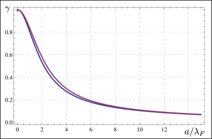
Figure 2: (Color online) The spin polarizability of a ferromagnetic cylinder and a sphere exceed the electrical polarizability by $\frac{\lambda_{\scriptscriptstyle N}}{\lambda_{\scriptscriptstyle F}}\gamma_{\scriptscriptstyle\textit{cyl}}$ and $\frac{\lambda_{\scriptscriptstyle N}}{\lambda_{\scriptscriptstyle F}}\gamma_{\scriptscriptstyle\textit{sphere}}$, respectively. The functions $\gamma_{\scriptscriptstyle\textit{cyl}}$ (blue) and $\gamma_{\scriptscriptstyle\textit{sphere}}$ (purple) are plotted versus the dimensionless radius, $a/\lambda_{\scriptscriptstyle F}$, from Eqs. (26), (31).

$${\bm{j}}^{\scriptscriptstyle N}({\bm{r}})={\bm{j}}^{\scriptscriptstyle 0}-{\bm{j}}^{\scriptscriptstyle 0}\frac{a^{3}}{r^{3}}+3a^{3}\frac{({\bm{j}}^{\scriptscriptstyle 0}\cdot{\bm{r}}){\bm{r}}}{r^{5}},$$ (28)

while the spin-current density distribution is given by

$${\bm{j}}^{\scriptscriptstyle N}_{s}({\bm{\rho}})={\bm{j}}^{\scriptscriptstyle 0}_{s}-\left(a^{3}\frac{\mathcal{P}_{\scriptscriptstyle\textit{sphere}}}{\mathcal{P}}\right)\left(\frac{{\bm{j}}^{\scriptscriptstyle 0}_{s}}{r^{3}}-3\frac{({\bm{j}}^{\scriptscriptstyle 0}_{s}\cdot{\bm{r}}){\bm{r}}}{r^{5}}\right),$$ (29)

where the induced spin-dipole moment has a form

$$\mathcal{P}_{\scriptscriptstyle\textit{sphere}}=\dfrac{\frac{3}{2}\sigma^{\scriptscriptstyle N}\dfrac{\sigma^{\scriptscriptstyle F}_{\scriptscriptstyle\uparrow}-\sigma^{\scriptscriptstyle F}_{\scriptscriptstyle\downarrow}}{\sigma^{\scriptscriptstyle F}_{\scriptscriptstyle\uparrow}\sigma^{\scriptscriptstyle F}_{\scriptscriptstyle\downarrow}}\gamma_{\scriptscriptstyle\textit{sphere}}}{1+2\dfrac{\sigma^{\scriptscriptstyle N}}{\sigma^{\scriptscriptstyle F}_{\scriptscriptstyle\uparrow}\sigma^{\scriptscriptstyle F}_{\scriptscriptstyle\downarrow}}\left(\dfrac{{\sigma^{\scriptscriptstyle F}_{\scriptscriptstyle\uparrow}}^{2}+{\sigma^{\scriptscriptstyle F}_{\scriptscriptstyle\downarrow}}^{2}}{\sigma^{\scriptscriptstyle F}_{\scriptscriptstyle\uparrow}+\sigma^{\scriptscriptstyle F}_{\scriptscriptstyle\downarrow}}\right)\gamma_{\scriptscriptstyle\textit{sphere}}.},$$ (30)

with $\gamma_{\scriptscriptstyle\textit{sphere}}$ defined as

$$\gamma_{\scriptscriptstyle\textit{sphere}}=\left(\frac{\lambda_{\scriptscriptstyle F}}{a}\frac{i_{1}\left[\dfrac{a}{\lambda_{\scriptscriptstyle F}}\right]}{i_{1}^{\prime}\left[\dfrac{a}{\lambda_{\scriptscriptstyle F}}\right]}\right).$$ (31)

Here $i_{1}(z)$ is the modified spherical Bessel function.

Numerically, the functions $\gamma_{\scriptscriptstyle\textit{cyl}}$ and $\gamma_{\scriptscriptstyle\textit{sphere}}$, plotted in Fig. 2, are practically identical. For $a\ll\lambda_{\scriptscriptstyle F}$, they are equal to $1$, suggesting that the spin polarization of current at the surface of a small cylinder or a small sphere is given by Eq. (9) with the geometrical factor, $\gamma$, equal to $1$ instead of $\lambda_{\scriptscriptstyle F}/\lambda_{\scriptscriptstyle N}$. For $a\gg\lambda_{\scriptscriptstyle F}$ both $\gamma_{\scriptscriptstyle\textit{cyl}}$ and $\gamma_{\scriptscriptstyle\textit{sphere}}$ fall off as $\lambda_{\scriptscriptstyle F}/a$ which correspond to $\gamma\sim\lambda_{\scriptscriptstyle F}/a$.

III Injection from an electrode with a curved interface

In this Section we will consider three toy models of spin injection through the interface of finite area. These models allow exact analytical treatment of a non-planar interface. They will help us later for the analysis of spin injection from a ferromagnet into a semiconductor in the presence of interface roughness.

III.1 “Radial” injection from a cylinder

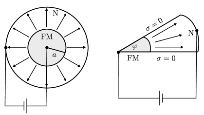
Figure 3: Schematic illustration of spin injection from a ferromagnet into a semiconductor in cylindrical and wedge geometries. The outside radii are much bigger than the radius, $a$, of the ferromagnetic core.

By cylindrical geometry we mean the arrangement of ferromagnet and semiconductor shown in Fig. 3a. The cross section of the ferromagnet is a circle with radius $a$. Most importantly, the current flows in the plane of the figure rather than along the axis of the cylinder, see Fig. 3a. Obviously, in this geometry, Eq. (1) should be solved in the polar coordinates. Namely, if we search for $\mu^{\scriptscriptstyle F}$ and $\mu^{\scriptscriptstyle N}$ in the form of the combination of harmonics, $\exp(im\theta)$, then the corresponding radial functions which ensure regular behavior at $\rho\rightarrow 0$ and at $\rho\rightarrow\infty$ are the modified Bessel functions $I_{m}$ and $K_{m}$, respectively. Thus we write

$$\mu_{\scriptscriptstyle\uparrow(\downarrow)}^{\scriptscriptstyle F} =\mu_{0}^{\scriptscriptstyle F}+\sum_{m}A_{\scriptscriptstyle m\uparrow(\downarrow)}I_{m}(\rho/\lambda_{\scriptscriptstyle F})e^{im\theta},$$ (32)

$$\mu_{\scriptscriptstyle\uparrow(\downarrow)}^{\scriptscriptstyle N} =\mu_{0}^{\scriptscriptstyle N}+\sum_{m}B_{\scriptscriptstyle m\uparrow(\downarrow)}K_{m}(\rho/\lambda_{\scriptscriptstyle N})e^{im\theta},$$ (33)

Here $\mu_{0}^{\scriptscriptstyle F}$ and $\mu_{0}^{\scriptscriptstyle N}$ are responsible for the non-polarized part of the current. Similar to the case of an embedded cylinder, the boundary conditions of the continuity of chemical potentials and radial currents should be imposed only on the amplitudes of harmonics. They assume the form

$$\left(A_{\scriptscriptstyle\uparrow}-A_{\scriptscriptstyle\downarrow}\right)I_{m}(a/\lambda_{\scriptscriptstyle F}) =\left(B_{\scriptscriptstyle\uparrow}-B_{\scriptscriptstyle\downarrow}\right)K_{m}(a/\lambda_{\scriptscriptstyle F}),$$ (34)

$$\frac{\sigma^{\scriptscriptstyle F}_{\scriptscriptstyle\uparrow}}{\lambda_{\scriptscriptstyle F}}I_{m}^{\prime}(a/\lambda_{\scriptscriptstyle F})A_{\scriptscriptstyle\uparrow} =\frac{\sigma^{\scriptscriptstyle N}}{\lambda_{\scriptscriptstyle N}}K_{m}^{\prime}(a/\lambda_{\scriptscriptstyle N})B_{\scriptscriptstyle\uparrow},$$ (35)

$$\frac{\sigma^{\scriptscriptstyle F}_{\scriptscriptstyle\downarrow}}{\lambda_{\scriptscriptstyle F}}I_{m}^{\prime}(a/\lambda_{\scriptscriptstyle F})A_{\scriptscriptstyle\downarrow} =\frac{\sigma^{\scriptscriptstyle N}}{\lambda_{\scriptscriptstyle N}}K_{m}^{\prime}(a/\lambda_{\scriptscriptstyle N})B_{\scriptscriptstyle\downarrow}.$$ (36)

It easily follows from the system Eq. (34) that, for any given $m$, the degree of polarization has a standard form Eq. (9) with the factor $\gamma$ replaced by $\gamma^{\scriptscriptstyle r}_{\scriptscriptstyle\textit{cyl}}$, which is defined as

$$\gamma^{\scriptscriptstyle r}_{\scriptscriptstyle\textit{cyl}}(m)=-\left(\frac{I_{m}(a/\lambda_{\scriptscriptstyle F})}{I^{\prime}_{m}(a/\lambda_{\scriptscriptstyle F})}\right)\left(\frac{K^{\prime}_{m}(a/\lambda_{\scriptscriptstyle N})}{K_{m}(a/\lambda_{\scriptscriptstyle N})}\right)\gamma.$$ (37)

Consider first the case $m=0$. Then Eq. (37) illustrates the main message formulated in the Introduction. Namely, when the perimeter, $2\pi a$, of the F/N boundary exceeds both $\lambda_{\scriptscriptstyle F}$ and $\lambda_{\scriptscriptstyle N}$, then the first ratio in Eq. (37) is equal to $1$, while the second ratio becomes $-1$, so that we get $\gamma^{\scriptscriptstyle r}_{\scriptscriptstyle\textit{cyl}}=\gamma$, i.e. the curvature of the boundary has no effect on injection.

Consider now an intermediate domain $\lambda_{\scriptscriptstyle F}\ll a\ll\lambda_{\scriptscriptstyle N}$. Then the argument in the first factor is big, while the argument in the second factor is small. Using the small-$z$ asymptote of $K_{0}(z)$ we find

$$\gamma^{\scriptscriptstyle r}_{\scriptscriptstyle\textit{cyl}}\Big{|}_{\lambda_{\scriptscriptstyle F}\ll a\ll\lambda_{\scriptscriptstyle N}}=\left(\frac{\lambda_{\scriptscriptstyle N}}{a\ln\frac{\lambda_{\scriptscriptstyle N}}{a}}\right)\frac{\lambda_{\scriptscriptstyle F}}{\lambda_{\scriptscriptstyle N}}=\frac{\lambda_{\scriptscriptstyle F}}{a\ln\frac{\lambda_{\scriptscriptstyle N}}{a}}.$$ (38)

We conclude that in the intermediate domain the injection efficiency is enhanced essentially by $\lambda_{\scriptscriptstyle N}/a$. Note that the above result matches, with logarithmic accuracy, the result Eq. (26) for the different geometry in which the external charge and spin currents flow not from, but rather through the ferromagnetic cylinder.

For a very small contact area $a\ll\lambda_{\scriptscriptstyle F}$ the arguments of the Bessel functions in both factors in Eq. (37) are small. From the asymptote $I_{0}(z)\approx 1+\frac{z^{2}}{4}$ we find

$$\gamma^{\scriptscriptstyle r}_{\scriptscriptstyle\textit{cyl}}\Big{|}_{a\ll\lambda_{\scriptscriptstyle F}\ll\lambda_{\scriptscriptstyle N}}=\left(\frac{2\lambda_{\scriptscriptstyle N}\lambda_{\scriptscriptstyle F}}{a^{2}\ln\frac{\lambda_{\scriptscriptstyle N}}{a}}\right)\frac{\lambda_{\scriptscriptstyle F}}{\lambda_{\scriptscriptstyle N}}\sim\frac{\lambda_{\scriptscriptstyle F}^{2}}{a^{2}}.$$ (39)

In the previous Section we have already realized that large spin diffusion length, $\lambda_{\scriptscriptstyle N}$, disappears from the injection efficiency. Eqs. (38), (39) essentially illustrate the same message and reaffirm the above picture that for large $\lambda_{\scriptscriptstyle N}$ the spin resistance of the semiconductor should be replaced by the spread resistance.

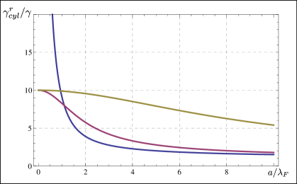
Figure 4: (Color online) The enhancement factor of the injected spin polarization is plotted for $\lambda_{\scriptscriptstyle N}=10\lambda_{\scriptscriptstyle F}$ from Eq. (37) versus the dimensionless radius, $a/\lambda_{\scriptscriptstyle F}$ of the ferromagnetic cylinder for angular momenta $m=0$ (blue), $m=1$ (purple), and $m=6$ (gold). The decay of the enhancement factor corresponds to $\frac{a}{\lambda_{\scriptscriptstyle F}}\sim m.$

For higher azimuthal harmonics, $m$, the enhancement of the injection efficiency is less pronounced as it is illustrated in Fig. 4. On the other hand, for larger $m$, the enhanced injection efficiency persists over a wider domain of the contact perimeters, $2\pi a$.

III.2 Injection in the wedge geometry

Additional insight into the geometrical enhancement of the spin injection can be inferred from the wedge-like arrangement of the F/N boundary illustrated in Fig. 3b. A novel feature present in Fig. 3b is that both the ferromagnetic injector and semiconductor are surrounded by vacuum with $\sigma=0$. Then in addition to the conditions Eqs. (2), (3) we must also require that the normal component of the current at the boundary with the vacuum is zero. This condition imposes the following angular dependence of the potentials,

$$\mu_{\scriptscriptstyle\uparrow}-\mu_{\scriptscriptstyle\downarrow}\sim\cos\frac{n\pi\theta}{\varphi},$$ (40)

where $\varphi$ is the opening angle of the wedge. It can be easily checked that the dependence Eq. (40) translates into the following form of the enhancement factor

$$\gamma_{\scriptscriptstyle\textit{wedge}}=-\left(\frac{I_{\frac{n\pi}{\varphi}}(a/\lambda_{\scriptscriptstyle F})}{I^{\prime}_{\frac{n\pi}{\varphi}}(a/\lambda_{\scriptscriptstyle F})}\right)\left(\frac{K^{\prime}_{\frac{n\pi}{\varphi}}(a/\lambda_{\scriptscriptstyle N})}{K_{\frac{n\pi}{\varphi}}(a/\lambda_{\scriptscriptstyle N})}\right)\gamma.$$ (41)

It is easy to see that the small opening angle, $\varphi$, is completely equivalent to the angular momentum $m=\frac{\pi}{\varphi}$ in Eq. (37). We have seen above that, for large $m$, the enhancement is $\frac{\lambda_{\scriptscriptstyle N}}{\lambda_{\scriptscriptstyle F}}$ and falls off with $a$ slowly, see Fig. 4. In this sense high values of $m$ are desirable, but the modes with high $m$ are hard to excite. The wedge geometry “simulates” high-$m$ values due to the small opening angle.

III.3 Injection with “size quantization”

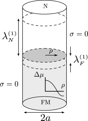
Figure 5: Schematic illustration of the size-quantization effect in spin injection. The modes, corresponding to oscillating distributions of $\Delta\mu$ in radial direction, decay along $x$ with decrements larger than $\lambda_{\scriptscriptstyle F}$ and $\lambda_{\scriptscriptstyle N}$, see Eqs. (43), (44). The behavior of $\Delta\mu(\rho)$ for $n=1$ is illustrated schematically.

In this subsection we study the enhancement of polarized injection for a more realistic situation when the ferromagnet and semiconducting materials contact each other over a finite area, $\pi a^{2}$, as illustrated in Fig. 5a. We restrict consideration to axisymmetric solutions, $m=0$. Then $\Delta\mu$, e.g. in ferromagnet, satisfies the equation

$$\frac{1}{\rho}\frac{\partial}{\partial\rho}\left(\rho\frac{\partial}{\partial\rho}\Delta\mu^{\scriptscriptstyle F}\right)+\frac{\partial^{2}}{\partial z^{2}}\Delta\mu^{\scriptscriptstyle F}=\frac{\Delta\mu^{\scriptscriptstyle F}}{\lambda^{2}_{\scriptscriptstyle F}}.$$ (42)

The enhancement in this geometry emerges from the fact that the condition of absence of current through the sides of the cylinder imposes “size quantization” of the radial dependencies of the chemical potentials $\mu^{\scriptscriptstyle F}$ and $\mu^{\scriptscriptstyle N}$. Namely, $\Delta\mu^{\scriptscriptstyle F}$ and $\Delta\mu^{\scriptscriptstyle N}$ behave with $\rho$ as a zero-order Bessel function, $J_{0}\left(\frac{\alpha\rho}{a}\right)$, where the constant $\alpha$ is fixed by absence of radial current at $\rho=a$, i.e. $J_{0}^{\prime}(\alpha)=0$. Thus the values of $\alpha$ are the roots, $\alpha_{1n}$, of the first-order Bessel function.

What is most important for the enhancement of the injection is that the solutions corresponding to different $n$ have different decay decrements along $z$. Indeed, from Eq. (42) we get

$$\left(\frac{1}{{\lambda^{\scriptscriptstyle(n)}_{\scriptscriptstyle F}}}\right)^{2}=\frac{1}{\lambda_{\scriptscriptstyle F}^{2}}+\frac{\alpha_{1n}^{2}}{a^{2}},$$ (43)

for the ferromagnet and similarly

$$\left(\frac{1}{\lambda^{\scriptscriptstyle(n)}_{\scriptscriptstyle N}}\right)^{2}=\frac{1}{\lambda_{\scriptscriptstyle N}^{2}}+\frac{\alpha_{1n}^{2}}{a^{2}},$$ (44)

for the semiconductor. The modification of $\lambda_{\scriptscriptstyle F}$ and $\lambda_{\scriptscriptstyle N}$ modifies the effective spin-resistances and thus the injection efficiency. This modification amounts to a replacement of $\lambda_{\scriptscriptstyle F}$, $\lambda_{\scriptscriptstyle N}$ in the geometrical factor $\gamma$ in Eq. (9) by $\lambda^{\scriptscriptstyle(n)}_{\scriptscriptstyle F}$ and $\lambda^{\scriptscriptstyle(n)}_{\scriptscriptstyle N}$, respectively. Overall we get

$$\gamma_{\scriptscriptstyle n}(a)=\left(\sqrt{\dfrac{a^{2}+\alpha_{1n}^{2}\lambda_{\scriptscriptstyle N}^{2}}{a^{2}+\alpha_{1n}^{2}\lambda_{\scriptscriptstyle F}^{2}}}\;\right)\gamma.$$ (45)

Again, for $a\gg\lambda_{\scriptscriptstyle F},\lambda_{\scriptscriptstyle N}$ we reproduce the infinite-area result $\gamma_{\scriptscriptstyle n}(a)=\gamma$. For $\lambda_{\scriptscriptstyle F}\ll a\ll\lambda_{\scriptscriptstyle N}$ the result becomes

$$\gamma_{\scriptscriptstyle n}(a)=\left(\frac{\alpha_{1n}\lambda_{\scriptscriptstyle N}}{a}\right)\gamma\sim\frac{\lambda_{\scriptscriptstyle F}}{a}.$$ (46)

Similar to Eq. (38) the largest spin-diffusion length $\lambda_{\scriptscriptstyle N}$ drops out of the spin-injection efficiency. In other words, the spin-resistance of the semiconductor is determined by a cylinder of diameter $a$ and height $\sim a$.

It is seen from Eq. (46) that the bigger is $n$ the stronger is the enhancement. On the other hand, similar to the solutions with high angular momentum, the solutions with large radial number are hard to excite. In the absence of inhomogeneity in the $\rho$-direction, the dominant solution is $\Delta\mu=\text{const}(\rho)$, and hence no enhancement of the injection.

IV Realistic geometries

IV.1 Rough interface: stalactites

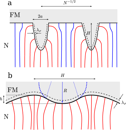
Figure 6: (Color online) Two models of a rough interface are depicted schematically; (a)interface roughness is modeled as a system of “stalactites” with surface density, $N$, and linear sizes $H$ and $a$. For $H\gg a$ the current is injected radially from the stalactite surface, so that the enhancement factor is given by Eq. (38). At distance $\sim H$ from the top of the stalactite the current distribution is homogeneous. (b) a model of an interface roughness with characteristic period, $H$, and amplitude $h\ll H$. Due to smallness of the ratio $h/H$ the characteristic radius of curvature $R=H^{2}/h$ is much bigger than $H$.

We will consider two models of the F/N interface roughness, see Fig. 6. In the first model the ferromagnet penetrates in a stalactite fashion into the semiconductor. We will assume that the height, $H$, and the diameter, $a$, of a typical stalactite is much bigger than $\lambda_{\scriptscriptstyle F}$ but much smaller than $\lambda_{\scriptscriptstyle N}$. We start from the simplest case $H=a$. It follows from the above consideration that even when the surface density, $N$, of stalactites is small, $Na^{2}\ll 1$ their presence might cause a strong net enhancement of the spin injection. As it was explained above, the origin of the enhancement is that for $\sigma_{\scriptscriptstyle\uparrow}^{\scriptscriptstyle F},\sigma_{\scriptscriptstyle\downarrow}^{\scriptscriptstyle F}\gg\sigma^{\scriptscriptstyle N}$ the force lines of electric field are normal to the curved F/N interface and the magnitude of the induced field decays at a scale $\sim a$ away from the interface. For the purposes of the spin injection it is also important that at distances from the stalactite surface also $\sim a$ the field lines become straight. This ensures that the contributions to the net spin polarization from the plane region of the interface and from the stalactites are additive. The last crucial observation is that, as long as the distance from the interface remains smaller than $\lambda_{\scriptscriptstyle N}$, the polarization of the current injected from the surface of the stalactite remains the same. Summarizing all the above arguments, we can present the average polarization as

$$\mathcal{P}_{\textit{injected}} =\mathcal{P}\left(1+N\frac{\mathcal{P}_{\scriptscriptstyle\textit{stal}}}{\mathcal{P}}a^{2}\right)$$ (47)

$$\approx\sigma^{\scriptscriptstyle N}\left(\frac{1}{\sigma^{\scriptscriptstyle F}_{\scriptscriptstyle\downarrow}}-\frac{1}{\sigma^{\scriptscriptstyle F}_{\scriptscriptstyle\uparrow}}\right)\frac{\lambda_{\scriptscriptstyle F}}{\lambda_{\scriptscriptstyle N}}\left(1+Na^{2}\frac{\gamma_{\scriptscriptstyle\textit{stal}}}{\gamma}\right),$$ (48)

where $\mathcal{P}_{\scriptscriptstyle\textit{stal}}$ and $\gamma_{\scriptscriptstyle\textit{stal}}$ in the second term in the brackets stand for the spin polarizability and the enhancement factor of the stalactite, respectively. In the case of a sphere and a cylinder, and all the cases considered thereafter, we obtained that, with accuracy of a numerical factor, the result for the enhancement factor is the same. For this reason we set $\gamma_{\scriptscriptstyle\textit{stal}}/{\gamma}\sim\lambda_{\scriptscriptstyle N}/a$. This leads us to the final result

$$\mathcal{P}_{\textit{injected}}=\sigma^{\scriptscriptstyle N}\left(\frac{1}{\sigma^{\scriptscriptstyle F}_{\scriptscriptstyle\downarrow}}-\frac{1}{\sigma^{\scriptscriptstyle F}_{\scriptscriptstyle\uparrow}}\right)\frac{\lambda_{\scriptscriptstyle F}}{\lambda_{\scriptscriptstyle N}}\left(1+Na\lambda_{\scriptscriptstyle N}\right).$$ (49)

It is seen from Eq. (49) that the stalactites dominate the injection when the distance between the neighbors is smaller than $(\lambda_{\scriptscriptstyle N}a)^{1/2}$. This condition is compatible with the assumption that this distance is bigger than $a$.

We now turn to the limit $H\gg a$. In this limit, the condition, $\sigma^{\scriptscriptstyle F}\gg\sigma^{\scriptscriptstyle N}$ leads to the field enhancement near the stalactite interface, in order to turn the field lines to from vertical to horizontal, see Fig. 6. As a result the polarized current is injected in the radial direction. Thus for $\lambda_{\scriptscriptstyle F}\ll a$ we can use Eq. (38) for the enhancement factor. Since the current from the stalactites is injected radially, while from the rest of the interface it is injected normally, it is convenient to calculate the average polarization using the cross section a distance $\sim H$ below the stalactites. Indeed, at a distance $\sim H$ below the stalactites the net current becomes homogeneous. A nontrivial element of the calculation is that, at such distances, the current lines, emanating from a given stalactite, occupy the area $\sim H^{2}$. In other words, the current injected from the area $2\pi aH$, which is the surface area of the stalactite, spreads out into the area $\sim H^{2}$. This is indeed the case, since, due to enhancement near the interface, the radial electric field exceeds the field away from the interface by $\sim H/a$. Basing on the above remarks, we conclude that the generalization of Eq. (47) to the case $H\gg a$ reads

$$\mathcal{P}_{\textit{injected}} =\mathcal{P}\left(1+N\frac{\mathcal{P}_{\scriptscriptstyle\textit{stal}}}{\mathcal{P}}H^{2}\right)$$ (50)

$$\approx\sigma^{\scriptscriptstyle N}\left(\frac{1}{\sigma^{\scriptscriptstyle F}_{\scriptscriptstyle\downarrow}}-\frac{1}{\sigma^{\scriptscriptstyle F}_{\scriptscriptstyle\uparrow}}\right)\frac{\lambda_{\scriptscriptstyle F}}{\lambda_{\scriptscriptstyle N}}\left(1+NH^{2}\frac{\gamma_{\scriptscriptstyle\textit{stal}}}{\gamma}\right).$$ (51)

Substituting $\gamma_{\textit{stal}}$ from Eq. (38), we arrive at the final result

$$\mathcal{P}_{\textit{injected}}=\sigma^{\scriptscriptstyle N}\left(\frac{1}{\sigma^{\scriptscriptstyle F}_{\scriptscriptstyle\downarrow}}-\frac{1}{\sigma^{\scriptscriptstyle F}_{\scriptscriptstyle\uparrow}}\right)\frac{\lambda_{\scriptscriptstyle F}}{\lambda_{\scriptscriptstyle N}}\left(1+N\frac{H^{2}\lambda_{\scriptscriptstyle N}}{a}\right).$$ (52)

Note that, while the condition $Na^{2}\ll 1$ ensures that the neighboring stalactites do not overlap, Eq. (52) is only valid for $N\lesssim 1/H^{2}$. The physical reason for this is that for higher densities the field enhancement takes place only within the distance $\sim N^{-1/2}$ from the tips of stalactites. This is because the stalactites screen the external field collectivelytubes . Thus for $N\gtrsim 1/H^{2}$ the result Eq. (52) saturates.

IV.2 Rough interface: small roughness amplitude

In the second model of a rough F/N interface the interface profile is sinusoidal, see Fig. 6 with characteristic amplitude, $h$, and the period, $H$. To find the $\gamma$-parameter, $\gamma_{\scriptscriptstyle\textit{sin}}$, for this model, we notice that the effective radius of curvature corresponding to a given element of the interface is $R=H^{2}/h$. As illustrated in Fig. 6b, one can view the injection from this element as a radial injection from the surface of a cylinder with radius $R$. This suggests that we can estimate $\gamma_{\scriptscriptstyle\textit{sin}}$ with the help of Eq. (38) in which the radius $a$ is replaced by $R$. This yields

$$\gamma_{\scriptscriptstyle\textit{sin}}\sim\frac{\lambda_{\scriptscriptstyle F}h}{H^{2}}.$$ (53)

The corresponding expression for polarization of the injected current reads

$$\mathcal{P}_{\scriptscriptstyle\textit{sin}}=\sigma^{\scriptscriptstyle N}\left(\frac{1}{\sigma^{\scriptscriptstyle F}_{\scriptscriptstyle\downarrow}}-\frac{1}{\sigma^{\scriptscriptstyle F}_{\scriptscriptstyle\uparrow}}\right)\frac{\lambda_{\scriptscriptstyle F}h}{H^{2}}.$$ (54)

Note that the result Eq. (38) pertained to the intermediate domain of the radii, $a$, namely $\lambda_{\scriptscriptstyle F}\ll a\ll\lambda_{\scriptscriptstyle N}$. With $a$ replaced by $R$, this domain turns out to be $(\lambda_{\scriptscriptstyle F}h)^{1/2}\ll H\ll(\lambda_{\scriptscriptstyle N}h)^{1/2}$. The first inequality suggests that $\gamma_{\scriptscriptstyle\textit{sin}}$ is small. As the period, $H$, gradually decreases and reaches $(\lambda_{\scriptscriptstyle F}a)^{1/2}$, the value $\gamma_{\scriptscriptstyle\textit{sin}}$ reaches $1$ and saturates upon further decrease of $H$.

IV.3 Injection via a ferromagnetic pillar

Assume that a ferromagnetic pillar of a radius, $a$, is in contact with a semiconductor surface, as shown in Fig. 7a. Since the conductivity in the lower half-space, except for the interior of the pillar is zero, the current lines near the interface between a semiconductor and non-conducting medium are almost horizontal. In general, the electric field inside the semiconductor behaves as a field of a charge distributed over the F/N interface. At distances $\gtrsim a$ from the contact this charge can be replaced by a point charge, so that electric field falls off with distance $r$ from the pillar as $1/r^{2}$. This knowledge is sufficient to deduce the electrical spread resistance of the contact to be $1/2\pi\sigma^{\scriptscriptstyle N}a$. Naturally, the spin resistance is the same. The spin resistance of the ferromagnet is calculated taking into account that the cross section area is $\pi a^{2}$, and the length is $\lambda_{\scriptscriptstyle F}$, yielding the value $\left(\frac{1}{\sigma^{\scriptscriptstyle F}_{\scriptscriptstyle\downarrow}}-\frac{1}{\sigma^{\scriptscriptstyle F}_{\scriptscriptstyle\uparrow}}\right)\frac{\lambda_{\scriptscriptstyle F}}{\pi a^{2}}.$ Then the spin polarization of the injected current calculated as a ratio of the two spin resistances reads

$$\mathcal{P}_{\scriptscriptstyle\textit{pillar}}=\sigma^{\scriptscriptstyle N}\left(\frac{1}{\sigma^{\scriptscriptstyle F}_{\scriptscriptstyle\downarrow}}-\frac{1}{\sigma^{\scriptscriptstyle F}_{\scriptscriptstyle\uparrow}}\right)\frac{\lambda_{\scriptscriptstyle F}}{2a}.$$ (55)

Note that this result is in line with the above expressions for $\mathcal{P}$, e.g. Eq. (38), if we treat $a$ as a radius of curvature. Like in previous examples, Eq. (55) applies when the ratio $\lambda_{\scriptscriptstyle F}/a$ is small. As $\lambda_{\scriptscriptstyle F}$ exceeds $a$, the ratio should be replaced by $1$.

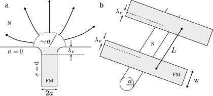
Figure 7: (a) Schematic illustration of spin injection through a nanopillar with radius $a\ll\lambda_{\scriptscriptstyle F}$. The force lines of electric field a curved within a distance $\sim a$ from the interface; (b) A typical nonlocal geometry employed for measurement of spin injection. Ferromagnetic injector and detector of width, w, are separated by distance, $L$, on top of a semiconduction wire with radius, $a$. It is presumed that the sizes are ordered as follows: $\lambda_{\scriptscriptstyle F}\ll a\ll\text{w}\ll L\ll\lambda_{\scriptscriptstyle N}$.

V discussion

• The main outcome of our study is that for a curved F/N interface the ratio $\lambda_{\scriptscriptstyle F}/\lambda_{\scriptscriptstyle N}$ in the seminal expression, Eq. (9), for the polarization of the injected current should be replaced by $\lambda_{\scriptscriptstyle F}/R$, where $R$ is the local curvature of the interface. Naturally, this replacement is appropriate when $R$ is smaller than $\lambda_{\scriptscriptstyle N}$.

  In our study we focused on a single F/N boundary. Note that, shortly after the publication of the paper Ref. wyder, , it was proposedSilsbeeTrueGeometry to measure the spin injection in a non-local geometry where the ferromagnetic injector and detector are spatially separated in the lateral direction. Nowadays this geometry is absolutely common in experimental studies of the spin transport, see e.g. recent papers Refs. InjectionIntoNanowire, ; vanWeesGrapheneInjection, ; LatestFertNonlocal, . At the same time, the theories, see e.g. Refs. CrossedGeometry1DCalculation, , Flatte-Yu, ; Hershfield, ; JapaneseInjection, , used to describe these non-local spin-injection setups are, essentially, “one-dimensional.” More specifically, they assume that the injection takes place along $x$ while the subsequent propagation of spin-polarization happens along $y$, so that these two processes are decoupled.

  To emphasize this point, in Fig. 7b. the nonlocal geometry is illustrated schematically, and all relevant sizes are indicated. Theories CrossedGeometry1DCalculation, , Flatte-Yu, ; Hershfield, ; JapaneseInjection, treat the injection in this geometry by dividing it into two F/N junctions in sequence. In particular the spin resistance of the wire part in Fig. 7b. is set to be proportionalCrossedGeometry1DCalculation to the wire length, $L$.

  We argue that such approach completely neglects the curving of the current paths upon injection from the ferromagnet into the wire, and that this curving changes dramatically the injected polarization. Our answer for this polarization contains $\lambda_{\scriptscriptstyle F}/\text{w}$ and does not depend on $L$. This is because the field lines turn 90 degrees over the distance $\sim\text{w}$, so that w plays the role of the radius of curvature.

  In fact, the importance of curving of the current paths in nonlocal geometry for for calculation of nonlocal electrical resistance was pointed out in Refs. JapaneseCurrentDistribution, , SilsbeeWire, .

• The idea that decreasing the contact area between a ferromagnet and a semiconductor can enhance the efficiency of the spin injection was previously expressed in Refs. GeomtericNanopillarTheory, , GeometricalEffectsTheory, . In particular, the geometry considered in Ref. GeomtericNanopillarTheory, was a ferromagnetic nanopillar with a radius $2\text{ nm}$. Numerical simulationsGeomtericNanopillarTheory suggest that constricting the injector to a small-radius cylinder leads to the enhancement of polarization from $10^{-3}\%$ to $\sim 1\%$ for certain parameters of a ferromagnet and semiconductor. Surprisingly, in interpreting the simulation results the authors of Ref. GeomtericNanopillarTheory, contend that the spread resistance suppresses the injection. In Ref. GeometricalEffectsTheory, the numerical simulations were also performed for a nanopillar-injector geometry. In addition to Ref. GeomtericNanopillarTheory, the authors traced a gradual enhancement of injection with decreasing the nanopillar area. However, another numerical finding reported in Ref. GeometricalEffectsTheory, , that the efficiency increases with increasing of the semiconductor thickness, seems counterintuitive.

• Experimental results of Ref. dali, seem to offer a partial support of our predictions. In Ref. dali, it was demonstrated that the performance of the vertical organic spin valves consisting of an organic layer of thickness $D\sim 100\text{ nm}$ sandwiched between two ferromagnets, $\text{Co}/\text{Alq}_{3}/\text{LSMO}$, can be significantly improved by covering the Co electrodes by a closely packed layer of Co nanodots. These nanodots represented spheres of a radius $\approx 1\text{ nm}$ which is smaller than $\lambda_{\scriptscriptstyle F}\approx 59\text{ nm}$ for Co, the value accepted in the literatureInjectionIntoNanowire . Incorporation of nanodots allowed the authors to increase the magnetoresistance from $\sim 10\%$ to $\sim 300\%$. Their explanation was that the layer of nanodots eliminates the “ill-defined” organic spacer layervaly1 ; valy2 . According to arguments presented above, the increase of injection efficiency due to the curvature of surface of nanodots is $\sim D/\lambda_{\scriptscriptstyle F}$.

VI Acknowledgements

We are grateful to Z. V. Vardeny for piquing our interest in the subject. This work was supported by NSF through MRSEC DMR-1121252.

References

• (1) P. C. van Son, H. van Kempen, and P. Wyder, Phys. Rev. Lett. 58, 2271 (1987).
• (2) F. J. Jedema, A. T. Filip, and B. J. van Wees, Nature (London) 410, 345 (2001).
• (3) M. Zaffalon and B. J. van Wees, Phys. Rev. Lett. 91, 186601 (2003).
• (4) F. J. Jedema, M. S. Nijboer, A. T. Filip, and B. J. van Wees, Phys. Rev. B 67, 085319 (2003).
• (5) V. P. LaBella, D. W. Bullock, Z. Ding, C. Emery, A. Venkatesan, W. F. Oliver, G. J. Salamo, P. M. Thibado, and M. Mortazavi, Science 292, 1518 (2001).
• (6) S. Heedt, C. Morgan, K. Weis, D. E. BΓΌrgler, R. Calarco, H. Hardtdegen, D. GrΓΌtzmacher, and T. SchΓ€pers, Nano Lett. 12, 4437 (2012).
• (7) D. GuimarΓ£es, A. Veligura, P. J. Zomer, T. Maassen, I. J. Vera-Marun, N. Tombros, and B. J. van Wees, Nano Lett. 12, 3512 (2012).
• (8) Y. Niimi, Y. Kawanishi, D. H. Wei, C. Deranlot, H. X. Yang, M. Chshiev, T. Valet, A. Fert, and Y. Otani, Phys. Rev. Lett. 109, 156602 (2012); Y. Niimi, H. Suzuki, Y. Kawanishi, Y. Omori, T. Valet, A. Fert, and Y. Otani, Phys. Rev. B 89, 054401 (2014).
• (9) R. Jansen, S. P. Dash, S. Sharma, and B. C. Min, Semicond. Sci. Technol. 27 083001 (2012).
• (10) G. Schmidt, D. Ferrand, L. W. Molenkamp, A. T. Filip, and B. J. van Wees, Phys. Rev. B 62, 790 (2000).
• (11) E. I. Rashba, Phys. Rev. B 62, 16267 (2000).
• (12) I. Zutic, J. Fabian, and S. Das Sarma, Rev. Mod. Phys. 76, 323 (2004).
• (13) S. A. Crooker, M. Furis, X. Lou, C. Adelmann, D. L. Smith, C. J. PalmstrΓΈm, and P. A. Crowell, Science 309, 2191 (2005).
• (14) X. Lou, C. Adelmann, S. A. Crooker, E. S. Garlid, J. Zhang, K. S. M. Reddy, S. D. Flexner, C. J. J. PalmstrΓΈm, and P. A. Crowell, Nat. Phys. 3, 197 (2007).
• (15) T. Valet and A. Fert, Phys. Rev. B 48, 7099 (1993).
• (16) M. Dzero, L. P. Gor kov, A. K. Zvezdin, and K. A. Zvezdin, Phys. Rev. B 67, 100402(R) (2003).
• (17) A. Khaetskii, J. C. Egues, D. Loss, C. Gould, G. Schmidt, and L. W. Molenkamp, Phys. Rev. B 71, 235327 (2005).
• (18) M. B. A. Jalil, S. G. Tan, S. Bala Kumar, and S. Bae, Phys. Rev. B 73, 134417 (2006).
• (19) J. M. Byers and M. E. FlattΓ©, Phys. Rev. Lett. 74, 306 (1995).
• (20) R. Lipperheide and U. Wille, Phys. Rev. B 72, 165322 (2005).
• (21) T. A. Sedrakyan, E. G. Mishchenko, and M. E. Raikh, Phys. Rev. B 73, 245325 (2006).
• (22) M. Johnson and R. H. Silsbee, Phys. Rev. B 37, 5312 (1988).
• (23) S. Hershfield and H.-L. Zhao, Phys. Rev. B 56, 3296 (1997).
• (24) Z. G. Yu and M. E. FlattΓ©, Phys. Rev. B 66, 201202 (2002).
• (25) S. Takahashi and S. Maekawa Phys. Rev. B 67, 052409 (2003).
• (26) J. Hamrle, T. Kimura, Y. Otani, K. Tsukagoshi, and Y. Aoyagi, Phys. Rev. B 71, 094402 (2005).
• (27) M. Johnson and R. H. Silsbee, Phys. Rev. B 76, 153107 (2007).
• (28) S. B. Kumar, S. G. Tan, M. B. A. Jalil, and J. Guo, Appl. Phys. Lett. 91, 142110 (2007).
• (29) J. Thingna and J.-S. Wang, J. Appl. Phys. 109, 12403 (2011).
• (30) D. Sun, L. Yin, C. Sun, H. Guo, Z. Gai, X.-G. Zhang, T. Z. Ward, Z. Cheng, and J. Shen, Phys. Rev. Lett. 104, 236602 (2010).
• (31) Z. H. Xiong, D. Wu, Z. V. Vardeny, and J. Shi, Nature 427, 821 (2004).
• (32) F. J. Wang, Z. H. Xiong, D. Wu, J. Shi, and Z. V. Vardeny, Synth. Met. 155, 172 (2005).