Underestimating extreme events in power-law behavior due to machine-dependent cutoffs
Abstract
Power-law distributions are typical macroscopic features occurring in almost all complex systems observable in nature, so that researchers have often the necessity, in quantitative analyses, to generate random synthetic variates obeying power-law distributions. The task is usually performed through standard methods that map uniform random variates into the desired probability space. Whereas all these algorithms are theoretically solid, in this paper we show that they are subjected to severe machine-dependent limitations. As results, two dramatic consequences arise: (i) the sampling in the tail of the distribution is not random but deterministic; (ii) the moments of the sample distribution, that are theoretically expected to diverge as functions of the sample sizes, converge instead to finite values. We provide quantitative indications for the range of distribution parameters that can be safely handled by standard libraries used in computational analyses. Whereas our findings indicate possible reinterpretations of numerical results obtained through flawed sampling methodologies, they also open the door for the search of a concrete solution to this central issue shared by all quantitative sciences dealing with complexity.
pacs:
89.75.-k, 89.75.Hc, 89.20.-aIf the probability to observe a particular value of some quantity is inversely proportional to the -th power of that value, i.e., , the quantity under observation is said to follow a power-law probability density function (pdf) or distribution. The first empirical observation of a power-law pdf dates back to the analysis by Pareto at the end of the s about the distribution of income and wealth among the population of Italy Moore (1897). Not so much after, Zipf noted that the frequency of any word in natural languages is inversely proportional to its rank in the frequency table Zipf (1949). Historically speaking, the contributions by Pareto and Zipf represented only the beginning of a long series of empirical discoveries of power-law distributions in natural and man-made systems. Thanks to the possibility offered by modern computational technologies to retrieve, store and analyze large-scale sets of data, the number of such empirical evidences has drastically increased in the last years, and is continuously growing. Power-law pdfs have been observed by researchers in almost all scientific disciplines, including physics Stanley (1987); Mandelbrot (1982); Barabási and Albert (1999), biology Viswanathan et al. (1996), earth and planetary sciences Gutenberg and Richter (1944); Boffetta et al. (1999), economics and finance Mantegna and Stanley (1995); Reed (2001); Gabaix (2008), computer science Faloutsos et al. (1999); Mitzenmacher (2004), and social science de Solla Price (1965); Brockmann et al. (2006), just to mention a few of them. For a recent review of power laws in empirical data see Clauset et al. (2009). Power-law distributions generally emerge in self-organized, critical, multiscale, and collective phenomena, and their ubiquity is interpreted as the consequence of the intrinsic complexity that drives the dynamics and organization of natural systems.
Computers play a fundamental role not only in the analysis of data, but they are also often used to run numerical simulations with the aim of understanding and possibly predicting the behavior of complex systems. Since power-law distributions are the emblematic features of complexity, computer simulations and analyses often rely on the construction of sequences of synthetic power-law variates, i.e., random numbers extracted from power-law distributions. Whereas the presence and consequences of serious numerical errors have been already studied in context of record statistics Wergen et al. (2012); Edery et al. (2013), so far none has questioned the effectiveness of the algorithms developed for the generation of power-law random variates. In this paper we show that all methods currently adopted for this purpose are instead subjected to severe machine-dependent limitations.
For simplicity, we will focus on the case of continuous random variates obeying the power-law pdf
| (1) |
if , and , otherwise. respectively indicate the upper and lower bounds of the support of , whereas is the exponent of the power-law distribution. The -th moment of the pdf of Eq. (1) is given by
| (2) |
valid for . For , we have instead . The previous equation mathematically formalizes a fundamental property of power-law distributions: all -th moments, with , diverge as powers (or logarithms) of the upper bound . The divergence of the moments of power-law pdfs is at the basis of many fundamental theoretical results. One requirement in the computer generation of power-law random numbers is thus to preserve this property. This task is, however, possible only under very restrictive conditions. Let us illustrate in details the origin of these numerical problems.
Suppose we want to create a sequence of computer-generated random variables extracted from the pdf of Eq. (1). Whereas there are many different ways to perform this task, here we will concentrate our attention on the so-called inversion method Devroye (1986); Clauset et al. (2009). We will come back to this point later, but we can already anticipate that the problems arising in the inversion method are common to all other methods that can be possibly be used to generate non uniform random variates. Our choice to focus on this method is not arbitrary, but motivated by its popularity in numerical analyses Clauset et al. (2009). The algorithm consists of two steps: (i) extract a random variable from a uniform distribution defined over the interval ; (ii) compute the random variate from the desired distribution by inverting the relation . While the approach is valid for any , it certainly results to be of great applicability in all cases in which the integral on the l.h.s. of the previous equation can be expressed explicitly, so that can be written in terms of . For power-law distributions , we can write
| (3) |
and use this relation to generate power-law distributed random variables directly from uniformly distributed random variates . Note that, in typical situations, so that Eq. (3) can be written as .
The inversion method is very elegant and theoretically solid, but, computationally speaking, it suffers of a severe weakness: its effectiveness relies on the goodness of the generator of random uniform variables. Generally, this fundamental role is played by pseudo-random number generators (PRNG). These are deterministic algorithms capable to produce high quality uniform variates with very long periods Devroye (1986); Matsumoto and Nishimura (1998). However, the precision at which these numbers are created is finite. Good PRNGs available on the market today have a precision of bits, meaning that the minimal distance between two random numbers generated by the PRNG is at maximum . While this precision is completely satisfactory for the generation of uniform random variates, when applied to the transformation of Eq. (3), it translates into a series of machine-dependent thresholds at which the distribution of the samples produced by the machine drastically diverges from the theoretical distribution .
The first problem that arises is the dramatic worsening of the accuracy at which random variates are extracted from . Suppose that we want to be able to discriminate between two consecutive random numbers with an accuracy equal to . This is possible only if the distance in the probability space between and is larger than . This requirement is firstly violated at , with defined by . When , the term of the l.h.s. can be approximated by the negative derivative of computed at . For power-law pdfs, we thus have
| (4) |
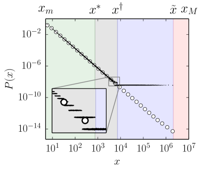
valid in the limit . For values of , power-law random variates are not longer extracted with the required accuracy . Consecutive admissible values differ by amounts larger than giving rise to a unwanted discretization (see Fig. 1). The most evident effect of the discretization is the presence of plateaus in the pdf of the samples. Plateaus are defined over overlapping intervals on the axis, and sudden jumps occur among consecutive plateaus. As increases, the discretization gets worse (i.e., plateaus become wider), until we reach the final plateau corresponding to a probability equal to . This level is reached for , where is defined by . For power-law pdfs, this means
| (5) |
valid for . The discretization of the probability and the sample space is certainly deleterious. The tail of the true distribution is not sampled at random, but in a deterministic fashion. No matter how many variables we extract, the sample pdf will never approach the true distribution, and particular values of will be never extracted. On the other hand, the consequences of this discretization on the effective divergence of the moments of the sample distribution are not as serious as those produced by the third threshold that we are going to describe.
Proceeding in the direction of increasing , an additional and much more severe threshold appears. Since no uniform numbers lower than can be extracted, there is no possibility to generate random variates from the distribution larger than defined by . For the special case of power-law pdfs, this machine-dependent cutoff in the sample pdf can be estimated as
| (6) |
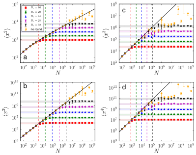
again valid for . The presence of a machine-dependent cutoff implies that the -th moment of the sample distribution behaves as .
For power-law pdfs with , the -th moment of the sample distribution, that is supposed to diverge as increases, instead converges to
| (7) |
A similar expression can be also found for .
To illustrate the practical importance of the machine-dependent limitations described so far, we present numerical evidences of problems induced by the finite precision PRNGs in two very common situations.
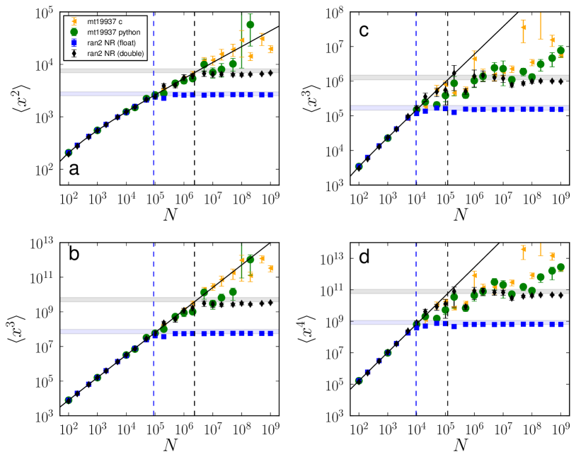
Fig. 2 illustrates the errors committed in a typical situation faced in the generation of random networks with prescribed degree distributions. These objects are generally constructed following the method developed by Molloy and Reed Molloy and Reed (1995). For a network with nodes, the first ingredient in the Molloy-Reed recipe consists in the creation of a degree sequence composed of random integers numbers extracted from an a priori fixed degree distribution, that, in the case of scale-free networks, consists in a list of random variables extracted from a power-law pdf defined over the interval , with generally set equal to . As it is well known, many fundamental results for random scale-free networks rely on the fact that the second moment of the degree distribution is divergent for any Barabási and Albert (1999); Albert and Barabási (2002); Dorogovtsev et al. (2008). Examples include the percolation threshold Cohen et al. (2000), the epidemic threshold Pastor-Satorras and Vespignani (2001), and the consensus time in the voter model Sood and Redner (2005). As Fig. 2 shows, however, the expected divergence of the moments of the degree distribution is numerically satisfied only up to values of , as predicted in Eq. (6). Results obtained with different PRNGs confirm that the precise value of the cutoffs can be machine- and implementation-dependent (see Fig. S1).
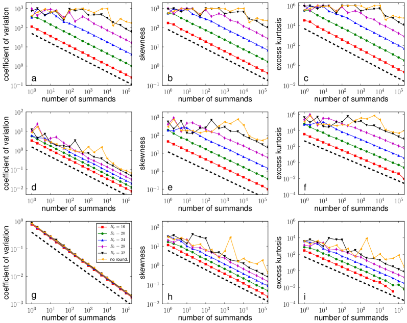
Our second example regards the statistics of the sum of power law random variables . This is a quantity of interest in many practical situations. For example, the total deformation of rock materials or of the Earth’s surface due to earthquakes may be modeled as the sum of seismic moment tensors Sotolongo-Costa et al. (2000); Kagan (2002), the latter obeying the Pareto distribution; cumulative economic losses or casualties due to natural catastrophes are modeled as sums of power-law distributed variables Voit (2003); the total pay-off of an insurance company is modeled as the sum of individual pay-offs, each of which is distributed according to a power law Kagan (1997). Also, the sum of random power-law variates plays an important role in superdiffusive processes modeled by Lévy flights, i.e., a special class of random walks in which the step-lengths obey a power-law probability distribution Shlesinger et al. (1993). Numerical simulations of Lévy flights are used in several contexts: for example, in the study of movements of animals and humans Viswanathan et al. (1996); Brockmann et al. (2006) and stochastic models of physical systems Shlesinger et al. (1995). Theory predicts two different behaviors for the sum of power-law random variables: for values of the power-law exponent , the pdf has finite variance, the central limit theorem applies, and the distribution of the sum approaches a normal distribution as the number of summands grows to infinity; for instead, has diverging variance, the generalized central limit theorem applies, and approaches a so-called -stable distribution as grows Nolan (2003); Zaliapin et al. (2005). The presence of the upper-bound in the distribution induces, however, catastrophic deviations from the expected behavior (see Fig. S2). For any value of the exponent there exists a maximal number of summands after which the distribution starts to show features typical of a normal distribution: coefficient of variation, skewness and excess kurtosis decrease to zero as the number of summands increases. This essentially means that if the number of summands is large enough, the distribution starts to become peaked and symmetric around a given value, as expected for a normal distribution. On the basis of the value of the machine-dependent cutoff of Eq. (6), we should expect to approach a normal distribution very slowly Mantegna and Stanley (1994). Our results, however, suggest that enters in a regime of “normality” for small values of the number of summands. For for example, the distribution starts to approach a normal distribution at when , and only for .
One may argue that the reason of the machine-dependent limitations illustrated so far resides only in the finite precision of the PNRG, so that the solution to this problem would be just to use a PRNG able to produce a number of random bits sufficiently large. Unfortunately, the solution is not as simple. When , as in the case of the orange points of Fig. 2, an additional machine-dependent effect may appear: the finite precision in the representation of numbers in our machine that affects the computation of powers. This second limitation approximately arises when we reach the so-called machine- or unit round off of our machine, i.e., the bits used in the so-called mantissa of the floating point number representation in the machine Goldberg (1991). Under the hypothesis of having a PRNG able to produce a number of random bits , the previous machine-dependent thresholds of Eqs. (4), (5) and (6) are still valid by substituting with . In our implementation, we have . This is however a limit that can be reached only if the PRNG is truly able to generate a sufficiently large number of random bits. The results of our simulations instead indicate that strong numerical inaccuracies arise earlier.
To summarize, the current implementations of the inversion method are not suitable for the generation of synthetic random variates obeying power-law distributions. Problems arise for the violation of two basic principles at the basis of the theory of this method: (i) there exists a perfect uniform random variate generator; (ii) computers can store and manipulate real numbers. The same principles are violated for any other method developed for the computer-generation of non uniform random variates, so that we expect to see similar problems also for other popular algorithms such as the rejection or the acceptance-complement methods Devroye (1986). In this paper, we explicitly considered the case of continuous random variates, but our results extend also to discrete variables. In addition, the same machine-dependent limitations hold for other pdfs rather than power-law distributions. For instance, exponential distributions are subjected to even stronger discretization effects. On the other hand, exponential pdfs have finite moments, and the presence of the machine-dependent cutoff causes errors not as dramatic as in the case of power laws or other heavy-tailed distributions.
The practical consequences of the existence of machine-dependent distortions in the computer generation of power-law random variates are diverse. For example, the discretization of random variables in the tail may be crucial for the outcome of tests of statistical significance of empirical data. The presence of a finite cutoff is certainly more dangerous. Finite size scaling analyses, for example, that do not account for it, are all potentially subjected to uncontrollable scaling factors. Even more seriously, in predictive analyses there is the concrete risk of underestimations of extreme events. Last but not least, since the limitations are machine-dependent neglecting their presence may cause problems of reproducibility of numerical experiments on different computers. The general and counter intuitive message of our analysis is that increasing the size of the sample does not improve the statistics, since in computer simulations fundamental properties of power-law distributions are preserved only up to relatively small sample sizes. With the current methodology, the only way to avoid all the numerical problems illustrated in this paper is to impose a forced cutoff at as defined in Eq. (4), reducing however the support of the pdf to incredibly small ranges. Future research must thus work on finding algorithms that do not suffer of this serious problem. In addition to more radical solutions based on the use of arbitrarily long numbers of bits in the representation of both uniform random numbers and powers, we believe that effective approaches could be based on generative models of power-law distributions Mitzenmacher (2004), features of dynamical systems Palatella and Grigolini (2012), or rely on the scale invariance property of powers.
References
- Moore (1897) H. Moore, The ANNALS of the American Academy of Political and Social Science 9, 128 (1897).
- Zipf (1949) G. Zipf, Human Behaviour and the Principle of Least-Effort (Addison-Wesley, Cambridge, MA, 1949).
- Stanley (1987) H. E. Stanley, Introduction to Phase Transitions and Critical Phenomena (Oxford University Press, USA, 1987).
- Mandelbrot (1982) B. Mandelbrot, The fractal geometry of nature (W.H. Freeman, 1982).
- Barabási and Albert (1999) A.-L. Barabási and R. Albert, science 286, 509 (1999).
- Viswanathan et al. (1996) G. M. Viswanathan, V. Afanasyev, S. V. Buldyrev, E. J. Murphy, P. A. Prince, and H. E. Stanley, Nature 381, 413 (1996).
- Gutenberg and Richter (1944) B. Gutenberg and C. Richter, Frequency of Earthquakes in California, Bulletin of the Seismological Society of America (Seismological Society of America, 1944).
- Boffetta et al. (1999) G. Boffetta, V. Carbone, P. Giuliani, P. Veltri, and A. Vulpiani, Physical Review Letters 83, 4662 (1999).
- Mantegna and Stanley (1995) R. N. Mantegna and H. E. Stanley, Nature 376, 46 (1995).
- Reed (2001) W. J. Reed, Economics Letters 74, 15 (2001).
- Gabaix (2008) X. Gabaix, Tech. Rep., National Bureau of Economic Research (2008).
- Faloutsos et al. (1999) M. Faloutsos, P. Faloutsos, and C. Faloutsos, in ACM SIGCOMM Computer Communication Review (ACM, 1999), vol. 29, pp. 251–262.
- Mitzenmacher (2004) M. Mitzenmacher, Internet Mathematics 1, 226 (2004).
- de Solla Price (1965) D. J. de Solla Price, Science 149, 510 (1965).
- Brockmann et al. (2006) D. Brockmann, L. Hufnagel, and T. Geisel, Nature 439, 462 (2006).
- Clauset et al. (2009) A. Clauset, C. R. Shalizi, and M. E. Newman, SIAM Review 51, 661 (2009).
- Wergen et al. (2012) G. Wergen, D. Volovik, S. Redner, and J. Krug, Phys. Rev. Lett. 109, 164102 (2012).
- Edery et al. (2013) Y. Edery, A. B. Kostinski, S. N. Majumdar, and B. Berkowitz, Phys. Rev. Lett. 110, 180602 (2013).
- Devroye (1986) L. Devroye, Non-Uniform Random Variate Generation (Springer-Verlag, 1986).
- Matsumoto and Nishimura (1998) M. Matsumoto and T. Nishimura, ACM Transactions on Modeling and Computer Simulation (TOMACS) 8, 3 (1998).
- Molloy and Reed (1995) M. Molloy and B. Reed, Random structures & algorithms 6, 161 (1995).
- Albert and Barabási (2002) R. Albert and A.-L. Barabási, Reviews of modern physics 74, 47 (2002).
- Dorogovtsev et al. (2008) S. N. Dorogovtsev, A. V. Goltsev, and J. F. Mendes, Reviews of Modern Physics 80, 1275 (2008).
- Cohen et al. (2000) R. Cohen, K. Erez, D. Ben-Avraham, and S. Havlin, Physical review letters 85, 4626 (2000).
- Pastor-Satorras and Vespignani (2001) R. Pastor-Satorras and A. Vespignani, Physical review letters 86, 3200 (2001).
- Sood and Redner (2005) V. Sood and S. Redner, Physical review letters 94, 178701 (2005).
- Sotolongo-Costa et al. (2000) O. Sotolongo-Costa, J. Antoranz, A. Posadas, F. Vidal, and A. Vazquez, Geophysical research letters 27, 1965 (2000).
- Kagan (2002) Y. Y. Kagan, Geophysical Journal International 149, 731 (2002).
- Voit (2003) J. Voit, The statistical mechanics of financial markets, vol. 2 (Springer Berlin, 2003).
- Kagan (1997) Y. Y. Kagan, Communications in statistics. Stochastic models 13, 775 (1997).
- Shlesinger et al. (1993) M. F. Shlesinger, G. M. Zaslavsky, and J. Klafter, Nature 363, 31 (1993).
- Shlesinger et al. (1995) M. F. Shlesinger, G. M. Zaslavsky, and U. Frisch, in Levy flights and related topics in Physics (1995), vol. 450.
- Nolan (2003) J. Nolan, Stable distributions: models for heavy-tailed data (Birkhauser, 2003).
- Zaliapin et al. (2005) I. Zaliapin, Y. Y. Kagan, and F. P. Schoenberg, Pure and Applied geophysics 162, 1187 (2005).
- Mantegna and Stanley (1994) R. N. Mantegna and H. E. Stanley, Physical Review Letters 73, 2946 (1994).
- Goldberg (1991) D. Goldberg, ACM Comput. Surv. 23, 5 (1991).
- Palatella and Grigolini (2012) L. Palatella and P. Grigolini, Physica A: Statistical Mechanics and its Applications 391, 5900 (2012).
- (38) Mersenne twister algorithm, URL http://www.math.sci.hiroshima-u.ac.jp/~m-mat/MT/emt.html.
- (39) GCC, the GNU compiler, URL http://gcc.gnu.org.
- Press et al. (2007) W. H. Press, S. A. Teukolsky, W. T. Vetterling, and B. P. Flannery, Numerical Recipes 3rd Edition: The Art of Scientific Computing (Cambridge University Press, New York, NY, USA, 2007).
Supplemental Material
Methods
To the best of our knowledge, the most efficient and accurate PRNG existing on the market is the Mersenne-Twister algorithm mt19937 developed by Matsumoto and Nishimura Matsumoto and Nishimura (1998). In our numerical simulations, we used the -bits version of mt19937 coded in c by the same inventors of the algorithm mt , compiled using the version of the gnu c compiler gcc . Simulations were run on -bits machines. To test the dependence of the machine-dependent cutoffs on the precision of the PRNG, we rounded the values produced by mt19937 to the desired number of bits . To further show how results are strongly machine- and/or implementation-dependent, in Fig. S1, we compared the results of Fig. 2 with those obtained using the default python PRNG, and the ran2 PRNG of numerical recipes Press et al. (2007).