Two-Term Disjunctions on the Second-Order Cone

Abstract

Balas introduced disjunctive cuts in the 1970s for mixed-integer linear programs. Several recent papers have attempted to extend this work to mixed-integer conic programs. In this paper we study the structure of the convex hull of a two-term disjunction applied to the second-order cone, and develop a methodology to derive closed-form expressions for convex inequalities describing the resulting convex hull. Our approach is based on first characterizing the structure of undominated valid linear inequalities for the disjunction and then using conic duality to derive a family of convex, possibly nonlinear, valid inequalities that correspond to these linear inequalities. We identify and study the cases where these valid inequalities can equivalently be expressed in conic quadratic form and where a single inequality from this family is sufficient to describe the convex hull. In particular, our results on two-term disjunctions on the second-order cone generalize related results on split cuts by Modaresi, Kılınç, and Vielma, and by Andersen and Jensen.

Keywords: Mixed-integer conic programming, second-order cone programming, cutting planes, disjunctive cuts

1 Introduction

A mixed-integer conic program is a problem of the form

$$\sup\{d^{\top}x:\;Ax=b,\;x\in\mathbb{K},\;x_{j}\in\mathbb{Z}\;\forall j\in J\}$$

where $\mathbb{K}\subset\mathbb{R}^{n}$ is a regular (full-dimensional, closed, convex, and pointed) cone, $A$ is an $m\times n$ real matrix, $d$ and $b$ are real vectors of appropriate dimensions, and $J\subseteq\{1,\ldots,n\}$. Mixed-integer conic programming (MICP) models arise naturally as robust versions of mixed-integer linear programming (MILP) models in finance, management, and engineering [11, 15]. MILP is the special case of MICP where $\mathbb{K}$ is the nonnegative orthant, and it has itself numerous applications. A successful approach to solving MILP problems has been to first solve the continuous relaxation, then add cuts, and finally perform branch-and-bound using this strengthened formulation. A powerful way of generating such cuts is to impose a valid disjunction on the continuous relaxation and derive tight convex inequalities for the resulting disjunctive set. Such inequalities are known as disjunctive cuts. Specifically, the integrality conditions on the variables $x_{j}$, $j\in J$, imply linear split disjunctions of the form $\pi^{\top}x\leq\pi_{0}\,\vee\,\pi^{\top}x\geq\pi_{0}+1$ where $\pi_{0}\in\mathbb{Z}$, $\pi_{j}\in\mathbb{Z}$, $j\in J$, and $\pi_{j}=0$, $j\not\in J$. Following this approach, the feasible region for MICP problems can be relaxed to $\{x\in\mathbb{K}:\,Ax=b,\pi^{\top}x\leq\pi_{0}\vee\pi^{\top}x\geq\pi_{0}+1\}$. More general two-term disjunctions arise in complementarity [23, 32] and other non-convex optimization [8, 16] problems. Therefore, it is interesting to study relaxations of MICP problems of the form

$$\sup\{d^{\top}x:\;x\in C_{1}\cup C_{2}\}\quad\text{where}$$

$$C_{i}:=\{x\in\mathbb{K}:\;Ax=b,\;c_{i}^{\top}x\geq c_{i,0}\}\quad\text{for}\quad i\in\{1,2\}$$ (1)

and to derive strong valid inequalities for the convex hull $\operatorname{conv}(C_{1}\cup C_{2})$, or the closed convex hull $\operatorname{\overline{conv}}(C_{1}\cup C_{2})$. When $\mathbb{K}$ is the nonnegative orthant, Bonami et al. [14] characterize $\operatorname{\overline{conv}}(C_{1}\cup C_{2})$ by a finite set of linear inequalities. The purpose of this paper is to study the structure of $\operatorname{\overline{conv}}(C_{1}\cup C_{2})$ for other cones such as the second-order (Lorentz) cone $\mathbb{K}_{2}^{n}:=\{x\in\mathbb{R}^{n}:\,\left\|(x_{1};\ldots;x_{n-1})\right\|_{2}\leq x_{n}\}$, or more generally the $p$-order cone $\mathbb{K}^{n}_{p}:=\{x\in\mathbb{R}^{n}:\,\left\|(x_{1};\ldots;x_{n-1})\right\|_{p}\leq x_{n}\}$ where $p\in(1,\infty)$, and provide the explicit description of $\operatorname{\overline{conv}}(C_{1}\cup C_{2})$ with convex inequalities in the space of the original variables. We first review related results from the literature.

Disjunctive cuts were introduced by Balas [4] for MILP in the early 1970s. Since then, disjunctive cuts have been studied extensively in mixed integer linear and nonlinear optimization [6, 30, 7, 19, 29, 17, 24, 16]. Chvátal-Gomory, lift-and-project, mixed-integer rounding (MIR), and split cuts are all special types of disjunctive cuts. Recent efforts on extending the cutting plane theory for MILP to the MICP setting include the work of Çezik and Iyengar [18] for Chvatal-Gomory cuts, Stubbs and Mehrotra [31], Drewes [21], Drewes and Pokutta [22], and Bonami [13] for lift-and-project cuts, and Atamtürk and Narayanan [2, 3] for MIR cuts. Kılınç-Karzan [25] analyzed properties of minimal valid linear inequalities for general conic sets with a disjunctive structure and showed that these are sufficient to describe the closed convex hull. Such general sets from [25] include two-term disjunctions on the cone $\mathbb{K}$ considered in this paper. Bienstock and Michalka [12] studied the characterization and separation of valid linear inequalities that convexify the epigraph of a convex, differentiable function restricted to a non-convex domain. In the last few years, there has been growing interest in developing closed-form expressions for convex inequalities that fully describe the convex hull of a disjunctive conic set. Dadush et al. [20] and Andersen and Jensen [1] derived split cuts for ellipsoids and the second-order cone, respectively. Modaresi et al. [26] extended this work on split disjunctions to essentially all cross-sections of the second-order cone, and studied their theoretical and computational relations with extended formulations and conic MIR inequalities in [27]. Belotti et al. [10] studied the families of quadratic surfaces having fixed intersections with two given hyperplanes and showed that these families can be described by a single parameter. Also, in [9], they identified a procedure for constructing two-term disjunctive cuts under the assumptions that $C_{1}\cap C_{2}=\emptyset$ and the sets $\{x\in\mathbb{K}:\,Ax=b,c_{1}^{\top}x=c_{1,0}\}$ and $\{x\in\mathbb{K}:\,Ax=b,c_{2}^{\top}x=c_{2,0}\}$ are bounded.

In this paper we study general two-term disjunctions on conic sets and give closed-form expressions for the tightest disjunctive cuts that can be obtained from these disjunctions in a large class of instances. We focus on the case where $C_{1}$ and $C_{2}$ in (1) above have an empty set of equations $Ax=b$. That is to say, we consider

$$C_{1}:=\{x\in\mathbb{K}:\,c_{1}^{\top}x\geq c_{1,0}\}\;\;\;\text{and}\;\;\;C_{2}:=\{x\in\mathbb{K}:\,c_{2}^{\top}x\geq c_{2,0}\}.$$ (2)

We note, however, that our results can easily be extended to two-term disjunctions on sets of the form $\{x\in\mathbb{R}^{n}:\,Ax-b\in\mathbb{K}\}$, where $A$ has full row rank, through the affine transformation discussed in [1]. Our main contribution is to give an explicit outer description of $\operatorname{\overline{conv}}(C_{1}\cup C_{2})$ when $\mathbb{K}$ is the second-order cone. Similar results have previously appeared in [1], [26], and [9]. Nevertheless, our work is set apart from [1] and [26] by the fact that we study two-term disjunctions on the cone $\mathbb{K}$ in their full generality and do not restrict our attention to split disjunctions, which are defined by parallel hyperplanes. Furthermore, unlike [9], we do not assume that $C_{1}\cap C_{2}=\emptyset$ and the sets $\{x\in\mathbb{K}:\,c_{1}^{\top}x=c_{1,0}\}$ and $\{x\in\mathbb{K}:\,c_{2}^{\top}x=c_{2,0}\}$ are bounded. In the absence of such assumptions, the resulting convex hulls turn out to be significantly more complex in our general setting. We also stress that our proof techniques originate from a conic duality perspective and are completely different from what is employed in the aforementioned papers; in particular, we believe that they are more intuitive in terms of their derivation, and more transparent in understanding the structure of the resulting convex hulls. Therefore, we hope that they have the potential to be instrumental in extending several important existing results in this growing area of research.

The remainder of this paper is organized as follows. Section 2 introduces the tools that will be useful to us in our analysis. In Section 2.1 we set out our notation and basic assumptions. In Section 2.2 we characterize the structure of undominated valid linear inequalities describing $\operatorname{\overline{conv}}(C_{1}\cup C_{2})$ when $\mathbb{K}$ is a regular cone. In Section 3 we focus on the case where $\mathbb{K}$ is the second-order cone. In Section 3.1 we state and prove our main result, Theorem 1. The proof uses conic duality, along with the characterization from Section 2.2, to derive a family of convex, possibly linear or conic, valid inequalities (8) for $\operatorname{\overline{conv}}(C_{1}\cup C_{2})$. In Sections 3.2 and 4, we identify and study the cases where these inequalities can equivalently be expressed in conic quadratic form and where only one inequality of the form (8) is sufficient to describe $\operatorname{\overline{conv}}(C_{1}\cup C_{2})$. Our results imply in particular that a single conic valid inequality is always sufficient for split disjunctions. Nevertheless, there are cases where it is not possible to obtain $\operatorname{\overline{conv}}(C_{1}\cup C_{2})$ with a single inequality of the form (8). In Section 5 we study those cases and outline a technique to characterize $\operatorname{\overline{conv}}(C_{1}\cup C_{2})$ with closed-form formulas. While the majority of our work is geared towards the second-order cone, in Section 6 we look at the $n$-dimensional $p$-order cone $\mathbb{K}_{p}^{n}$ with $p\in(1,\infty)$ and study elementary split disjunctions on this set. That is, we consider sets $C_{1}$ and $C_{2}$ defined as in (2) where $c_{1}$ and $c_{2}$ are multiples of the $i^{\text{th}}$ standard unit vector, $e^{i}$, $i\in\{1,\ldots,n-1\}$. We show that one can obtain a single conic inequality that describes the convex hull using our framework in this setup. This provides an alternative proof of a similar result by Modaresi et al. [26].

2 Preliminaries

The main purpose of this section is to characterize the structure of undominated valid linear inequalities for $\operatorname{\overline{conv}}(C_{1}\cup C_{2})$ when $\mathbb{K}$ is a regular cone and $C_{1}$ and $C_{2}$ are defined as in (2). First, we present our notation and assumptions.

2.1 Notation and Assumptions

Given a set $S\subseteq\mathbb{R}^{n}$, we let $\operatorname{span}S$, $\operatorname{int}S$, and $\operatorname{bd}S$ denote the linear span, interior, and boundary of $S$, respectively. We use $\operatorname{rec}S$ to refer to the recession cone of a convex set $S$. The dual cone of $\mathbb{K}\subseteq\mathbb{R}^{n}$ is $\mathbb{K}^{*}:=\{y\in\mathbb{R}^{n}:\,y^{\top}x\geq 0\,\forall x\in\mathbb{K}\}$. Recall that the dual cone $\mathbb{K}^{*}$ of a regular cone $\mathbb{K}$ is also regular and the dual of $\mathbb{K}^{*}$ is $\mathbb{K}$ itself.

We can always scale the inequalities $c_{1}^{\top}x\geq c_{1,0}$ and $c_{2}^{\top}x\geq c_{2,0}$ defining the disjunction so that their right-hand sides are $0$ or $\pm 1$. Therefore, from now on we assume that $c_{1,0},c_{2,0}\in\{0,\pm 1\}$ for notational convenience.

When $C_{1}\subseteq C_{2}$, we have $\operatorname{\overline{conv}}(C_{1}\cup C_{2})=C_{2}$. Similarly, when $C_{1}\supseteq C_{2}$, we have $\operatorname{\overline{conv}}(C_{1}\cup C_{2})=C_{1}$. In the remainder we focus on the case where $C_{1}\not\subseteq C_{2}$ and $C_{1}\not\supseteq C_{2}$.

Assumption 1.

$C_{1}\not\subseteq C_{2}$ and $C_{1}\not\supseteq C_{2}$.

In particular, Assumption 1 implies $c_{i}\not\in-\mathbb{K}^{*}$ when $c_{i,0}=+1$ and $c_{i}\not\in\mathbb{K}^{*}$ when $c_{i,0}=-1$. We also need the following technical assumption in our analysis.

Assumption 2.

$C_{1}$ and $C_{2}$ are strictly feasible sets. That is, $C_{1}\cap\operatorname{int}\mathbb{K}\neq\emptyset$ and $C_{2}\cap\operatorname{int}\mathbb{K}\neq\emptyset$.

The set $C_{i}$ is always strictly feasible when it is nonempty and $c_{i,0}\in\{\pm 1\}$. Therefore, we need Assumption 2 to supplement Assumption 1 only when $c_{1,0}=0$ or $c_{2,0}=0$. Note that, under Assumption 2, the sets $C_{1}$ and $C_{2}$ always have nonempty interior. Assumptions 1 and 2 have several simple implications, which we state next. The first lemma extends ideas from Balas [5] to disjunctions on more general convex sets. Its proof is left to the appendix.

Lemma 1.

Let $S\subset\mathbb{R}^{n}$ be a closed, convex, pointed set, $S_{1}:=\{x\in S:\,c_{1}^{\top}x\geq c_{1,0}\}$, and $S_{2}:=\{x\in S:\,c_{2}^{\top}x\geq c_{2,0}\}$ for $c_{1},c_{2}\in\mathbb{R}^{n}$ and $c_{1,0},c_{2,0}\in\mathbb{R}$. Suppose $S_{1}\not\subseteq S_{2}$ and $S_{1}\not\supseteq S_{2}$. Then

1. $S_{1}\cup S_{2}$ is not convex unless $S_{1}\cup S_{2}=S$,

2. $\operatorname{\overline{conv}}(S_{1}\cup S_{2})=\operatorname{conv}(S_{1}^{+}\cup S_{2}^{+})$ where $S_{1}^{+}:=S_{1}+\operatorname{rec}S_{2}$ and $S_{2}^{+}:=S_{2}+\operatorname{rec}S_{1}$.

Clearly, when $\operatorname{\overline{conv}}(C_{1}\cup C_{2})\neq\mathbb{K}$, we do not need to derive any new inequalities to get a description of the closed convex hull. The next lemma obtains a natural consequence of Assumption 1 through conic duality.

Lemma 2.

Consider $C_{1},C_{2}$ defined as in (2). Suppose Assumption 1 holds. Then the following system of inequalities in the variable $\beta$ is inconsistent:

$$\beta\geq 0,\quad\beta c_{1,0}\geq c_{2,0},\quad c_{2}-\beta c_{1}\in\mathbb{K}^{*}.$$ (3)

Similarly, the following system of inequalities in the variable $\beta$ is inconsistent:

$$\beta\geq 0,\quad\beta c_{2,0}\geq c_{1,0},\quad c_{1}-\beta c_{2}\in\mathbb{K}^{*}.$$ (4)

Proof.

Suppose there exists $\beta^{*}$ satisfying (3). For all $x\in\mathbb{K}$, this implies $(c_{2}-\beta^{*}c_{1})^{\top}x\geq 0\geq c_{2,0}-\beta^{*}c_{1,0}$. Then any point $x\in C_{1}$ satisfies $\beta^{*}c_{1}^{\top}x\geq\beta^{*}c_{1,0}$ and therefore, $c_{2}^{\top}x\geq c_{2,0}$. Hence, $C_{1}\subseteq C_{2}$ which contradicts Assumption 1. The proof for the inconsistency of (4) is similar.∎

2.2 Properties of Undominated Valid Linear Inequalities

A valid linear inequality $\mu^{\top}x\geq\mu_{0}$ for a feasible set $S\subseteq\mathbb{K}$ is said to be tight if $\inf_{x}\{\mu^{\top}x:\,x\in S\}=\mu_{0}$ and strongly tight if there exists $x^{*}\in S$ such that $\mu^{\top}x^{*}=\mu_{0}$.

A valid linear inequality $\nu^{\top}x\geq\nu_{0}$ for a strictly feasible set $S\subseteq\mathbb{K}$ is said to dominate another valid linear inequality $\mu^{\top}x\geq\mu_{0}$ if it is not a positive multiple of $\mu^{\top}x\geq\mu_{0}$ and implies $\mu^{\top}x\geq\mu_{0}$ together with the cone constraint $x\in\mathbb{K}$. Furthermore, a valid linear inequality $\mu^{\top}x\geq\mu_{0}$ is said to be undominated if there does not exists another valid linear inequality $\nu^{\top}x\geq\nu_{0}$ such that $(\mu-\nu,\mu_{0}-\nu_{0})\in\mathbb{K}^{*}\times-\mathbb{R}_{+}\setminus\{(0,0)\}$. This notion of domination is closely tied with the $\mathbb{K}$-minimality definition of [25] which says that a valid linear inequality $\mu^{\top}x\geq\mu_{0}$ is $\mathbb{K}$-minimal if there does not exist another valid linear inequality $\nu^{\top}x\geq\nu_{0}$ such that $(\mu-\nu,\mu_{0}-\nu_{0})\in(\mathbb{K}^{*}\setminus\{0\})\times-\mathbb{R}_{+}$. In particular, a valid linear inequality for $\operatorname{\overline{conv}}(C_{1}\cup C_{2})$ is undominated in the sense considered here if and only if it is $\mathbb{K}$-minimal and tight on $\operatorname{\overline{conv}}(C_{1}\cup C_{2})$. In [25], $\mathbb{K}$-minimal inequalities are defined and studied for sets of the form

$$\left\{x\in\mathbb{R}^{n}:\,Ax\in H,\,x\in\mathbb{K}\right\},$$

where $H$ is an arbitrary set and $\mathbb{K}$ is a regular cone. Our set $C_{1}\cup C_{2}$ can be represented in the form above as

$$\left\{x\in\mathbb{R}^{n}:\,\begin{pmatrix}c_{1}^{T}\\ c_{2}^{T}\end{pmatrix}x=\left\{{\{c_{1,0}\}+\mathbb{R}_{+}\choose\mathbb{R}}\right\}\bigcup\left\{{\mathbb{R}\choose\{c_{2,0}\}+\mathbb{R}_{+}}\right\},~{}x\in\mathbb{K}\right\}.$$

Because $C_{1}\cup C_{2}$ is full-dimensional under Assumption 2, Proposition 1 of [25] can be used to conclude that the extreme rays of the convex cone of valid linear inequalities

$$M:=\left\{(\mu,\mu_{0})\in\mathbb{R}^{n}\times\mathbb{R}:\;\mu^{\top}x\geq\mu_{0}\;\forall x\in\operatorname{\overline{conv}}(C_{1}\cup C_{2})\right\}$$

are either tight, $\mathbb{K}$-minimal inequalities or implied by the cone constraint $x\in\mathbb{K}$. Hence, one needs to add only undominated valid linear inequalities to the cone constraint $x\in\mathbb{K}$ to obtain an outer description of $\operatorname{\overline{conv}}(C_{1}\cup C_{2})$.

Because $C_{1}$ and $C_{2}$ are strictly feasible sets by Assumption 2, conic duality implies that a linear inequality $\mu^{\top}x\geq\mu_{0}$ is valid for $\operatorname{\overline{conv}}(C_{1}\cup C_{2})$ if and only if there exist $\alpha_{1},\alpha_{2},\beta_{1},\beta_{2}$ such that $(\mu,\mu_{0},\alpha_{1},\alpha_{2},\beta_{1},\beta_{2})$ satisfies

$$\begin{gathered}\mu=\alpha_{1}+\beta_{1}c_{1},\\ \mu=\alpha_{2}+\beta_{2}c_{2},\\ \beta_{1}c_{1,0}\geq\mu_{0},\quad\beta_{2}c_{2,0}\geq\mu_{0},\\ \alpha_{1},\alpha_{2}\in\mathbb{K}^{*},\quad\beta_{1},\beta_{2}\in\mathbb{R}_{+}.\end{gathered}$$ (5)

This system can be reduced slightly when we consider undominated valid linear inequalities.

Proposition 1.

Consider $C_{1},C_{2}$ defined as in (2) with $c_{1,0},c_{2,0}\in\{0,\pm 1\}$. Suppose Assumptions 1 and 2 hold. Then, up to positive scaling, any undominated valid linear inequality for $\operatorname{\overline{conv}}(C_{1}\cup C_{2})$ has the form $\mu^{\top}x\geq\min\{c_{1,0},c_{2,0}\}$ with $(\mu,\alpha_{1},\alpha_{2},\beta_{1},\beta_{2})$ satisfying

$$\begin{gathered}\mu=\alpha_{1}+\beta_{1}c_{1},\\ \mu=\alpha_{2}+\beta_{2}c_{2},\\ \min\{\beta_{1}c_{1,0},\beta_{2}c_{2,0}\}=\min\{c_{1,0},c_{2,0}\},\\ \alpha_{1},\alpha_{2}\in\operatorname{bd}\mathbb{K}^{*},\quad\beta_{1},\beta_{2}\in\mathbb{R}_{+}\setminus\{0\}.\end{gathered}$$ (6)

Proof.

Let $\nu^{\top}x\geq\nu_{0}$ be a valid inequality for $\operatorname{\overline{conv}}(C_{1}\cup C_{2})$. Then there exist $\alpha_{1},\alpha_{2},\beta_{1},\beta_{2}$ such that $(\nu,\nu_{0},\alpha_{1},\alpha_{2},\beta_{1},\beta_{2})$ satisfies (5). If $\beta_{1}=0$ or $\beta_{2}=0$, then $\nu^{\top}x\geq\nu_{0}$ is implied by the cone constraint $x\in\mathbb{K}$. If $\min\{\beta_{1}c_{1,0},\beta_{2}c_{2,0}\}>\nu_{0}$, then $\nu^{\top}x\geq\nu_{0}$ is implied by the valid inequality $\nu^{\top}x\geq\min\{\beta_{1}c_{1,0},\beta_{2}c_{2,0}\}$. Hence, we can assume without any loss of generality that any undominated valid linear inequality for $\operatorname{\overline{conv}}(C_{1}\cup C_{2})$ has the form $\nu^{\top}x\geq\nu_{0}$ with $(\nu,\nu_{0},\alpha_{1},\allowbreak\alpha_{2},\beta_{1},\beta_{2})$ satisfying

$$\begin{gathered}\nu=\alpha_{1}+\beta_{1}c_{1},\\ \nu=\alpha_{2}+\beta_{2}c_{2},\\ \min\{\beta_{1}c_{1,0},\beta_{2}c_{2,0}\}=\nu_{0}\\ \alpha_{1},\alpha_{2}\in\mathbb{K}^{*},\;\beta_{1},\beta_{2}\in\mathbb{R}_{+}\setminus\{0\}.\end{gathered}$$

We are now going to show that when $\alpha_{1}\in\operatorname{int}\mathbb{K}^{*}$ or $\alpha_{2}\in\operatorname{int}\mathbb{K}^{*}$, any such inequality is either dominated or equivalent to a valid inequality $\mu^{\top}x\geq\min\{c_{1,0},c_{2,0}\}$ that satisfies (6). Assume without any loss of generality that $\alpha_{2}\in\operatorname{int}\mathbb{K}^{*}$. There are two cases that we need to consider: $\alpha_{1}=0$ and $\alpha_{1}\neq 0$.

First suppose $\alpha_{1}=0$. We have $\alpha_{2}=\beta_{1}c_{1}-\beta_{2}c_{2}\in\operatorname{int}\mathbb{K}^{*}$. By Lemma 2 and taking $\beta_{1},\beta_{2}>0$ into account, we conclude $\beta_{2}c_{2,0}<\beta_{1}c_{1,0}$. Hence, $\nu_{0}=\beta_{2}c_{2,0}$. If $\nu_{0}>0$, let $0<\epsilon^{\prime}<\beta_{1}$ be such that $\alpha_{2}^{\prime}:=\alpha_{2}-\epsilon^{\prime}c_{1}\in\mathbb{K}^{*}$ and $\beta_{2}c_{2,0}\leq\beta_{1}c_{1,0}-\epsilon^{\prime}c_{1,0}$ and define $\beta_{1}^{\prime}:=\beta_{1}-\epsilon^{\prime}$ and $\mu:=\nu-\epsilon^{\prime}c_{1}$. If $\nu_{0}\leq 0$, let $\epsilon^{\prime}>0$ be such that $\alpha_{2}^{\prime}:=\alpha_{2}+\epsilon^{\prime}c_{1}\in\mathbb{K}^{*}$ and $\beta_{2}c_{2,0}\leq\beta_{1}c_{1,0}+\epsilon^{\prime}c_{1,0}$ and define $\beta_{1}^{\prime}:=\beta_{1}+\epsilon^{\prime}$ and $\mu:=\nu+\epsilon^{\prime}c_{1}$. In either case, the inequality $\mu^{\top}x\geq\nu_{0}$ is valid for $\operatorname{\overline{conv}}(C_{1}\cup C_{2})$ because $(\mu,\nu_{0},\alpha_{1},\alpha_{2}^{\prime},\beta_{1}^{\prime},\beta_{2})$ satisfies (5). Furthermore, it dominates (or in the case of $\nu_{0}=0$, is equivalent to) $\nu^{\top}x\geq\nu_{0}$ because $\mu=\frac{\beta_{1}^{\prime}}{\beta_{1}}\nu$ and $\beta_{1}^{\prime}<\beta_{1}$ when $\nu_{0}>0$ and $\beta_{1}^{\prime}>\beta_{1}$ when $\nu_{0}\leq 0$.

Now suppose $\alpha_{1}\neq 0$. Let $0<\epsilon^{\prime\prime}\leq 1$ be such that $\alpha_{2}^{\prime\prime}:=\alpha_{2}-\epsilon^{\prime\prime}\alpha_{1}\in\operatorname{bd}\mathbb{K}^{*}$, and define $\alpha_{1}^{\prime\prime}:=(1-\epsilon^{\prime\prime})\alpha_{1}$ and $\mu:=\nu-\epsilon^{\prime\prime}\alpha_{1}$. The inequality $\mu^{\top}x\geq\nu_{0}$ is valid for $\operatorname{\overline{conv}}(C_{1}\cup C_{2})$ because $(\mu,\nu_{0},\alpha_{1}^{\prime\prime},\alpha_{2}^{\prime\prime},\beta_{1},\beta_{2})$ satisfies (5). Furthermore, $\mu^{\top}x\geq\nu_{0}$ dominates $\nu^{\top}x\geq\nu_{0}$ since $\nu-\mu=\epsilon^{\prime\prime}\alpha_{1}\in\mathbb{K}^{*}\setminus\{0\}$.

Finally, note that we can scale any valid inequality $\mu^{\top}x\geq\nu_{0}$ (along with the tuple $(\mu,\nu_{0},\alpha_{1},\alpha_{2},\beta_{1},\beta_{2})$) so that $\nu_{0}\in\{0,\pm 1\}$. Using the fact that $\beta_{1},\beta_{2}>0$ in an undominated valid inequality, we arrive at

$$\nu_{0} =\operatorname{sign}(\nu_{0})=\operatorname{sign}(\min\{\beta_{1}c_{1,0},\beta_{2}c_{2,0}\})$$

$$=\min\{\underbrace{\operatorname{sign}(\beta_{1}c_{1,0})}_{=\operatorname{sign}(c_{1,0})},\underbrace{\operatorname{sign}(\beta_{2}c_{2,0})}_{=\operatorname{sign}(c_{2,0})}\}=\min\{c_{1,0},c_{2,0}\}.$$

∎

Remark.

Under the assumptions of Proposition 1, in an undominated valid linear inequality $\mu^{\top}x\geq\min\{c_{1,0},c_{2,0}\}$, we can assume that at least one of $\beta_{1}$ and $\beta_{2}$ is equal to $1$ in (6) without any loss of generality. In particular,

1. if $c_{1,0}>c_{2,0}$, we can assume that $\beta_{2}=1$, $\beta_{1}c_{1,0}\geq c_{2,0}$, and $\beta_{1}c_{1}-c_{2}\notin\pm\operatorname{int}\mathbb{K}^{*}$ holds,

2. if $c_{1,0}=c_{2,0}$, we can assume that either $\beta_{2}=1$, $\beta_{1}c_{1,0}\geq c_{2,0}$, and $\beta_{1}c_{1}-c_{2}\notin\pm\operatorname{int}\mathbb{K}^{*}$ or $\beta_{1}=1$, $\beta_{2}c_{2,0}\geq c_{1,0}$, and $\beta_{2}c_{2}-c_{1}\notin\pm\operatorname{int}\mathbb{K}^{*}$ holds.

Proof.

The remark follows from a careful look at the proof of Proposition 1.

First suppose $c_{1,0}>c_{2,0}$. In this case the equality $\min\{\beta_{1}c_{1,0},\beta_{2}c_{2,0}\}=\min\{c_{1,0},c_{2,0}\}$ reduces to $\beta_{2}c_{2,0}=c_{2,0}$ since $\operatorname{sign}(\beta_{1}c_{1,0})=c_{1,0}>c_{2,0}=\operatorname{sign}(\beta_{2}c_{2,0})$. This already implies $\beta_{2}=1$ when $c_{2,0}\in\{\pm 1\}$. When $c_{2,0}=0$, any undominated valid linear inequality has the form $\mu^{\top}x\geq 0$ and we can scale this inequality (along with the tuple $(\mu,\alpha_{1},\alpha_{2},\beta_{1},\beta_{2})$ that satisfies (6)) by a positive scalar to obtain an equivalent valid inequality with $\beta_{2}=1$. Therefore, when $c_{1,0}>c_{2,0}$, any undominated valid linear inequality for $\operatorname{\overline{conv}}(C_{1}\cup C_{2})$ has the form $\mu^{\top}x\geq c_{2,0}$ with $(\mu,\alpha_{1},\alpha_{2},\beta)$ satisfying the system

$$\begin{gathered}\mu=\alpha_{1}+\beta c_{1},\\ \mu=\alpha_{2}+c_{2},\\ \alpha_{1},\alpha_{2}\in\operatorname{bd}\mathbb{K}^{*},\;\beta\in\mathbb{R}_{+}\setminus\{0\}.\end{gathered}$$

In particular, this implies $c_{2}-\beta c_{1}\notin\operatorname{int}\mathbb{K}^{*}$ since we must have $\alpha_{1}=\alpha_{2}+(c_{2}-\beta c_{1})\in\operatorname{bd}\mathbb{K}^{*}$ and $c_{2}-\beta c_{1}\notin-\operatorname{int}\mathbb{K}^{*}$ since we must have $\alpha_{2}=\alpha_{1}-(c_{2}-\beta c_{1})\in\operatorname{bd}\mathbb{K}^{*}$.

Now suppose $c_{1,0}=c_{2,0}$. In this case the equality $\min\{\beta_{1}c_{1,0},\beta_{2}c_{2,0}\}=\min\{c_{1,0},c_{2,0}\}$ becomes $\min\{\beta_{1}c_{1,0},\beta_{2}c_{2,0}\}=c_{1,0}=c_{2,0}$. When $c_{1,0}=c_{2,0}\in\{\pm 1\}$, this implies either $\beta_{1}=1$ or $\beta_{2}=1$. Otherwise, any undominated valid linear inequality has the form $\mu^{\top}x\geq 0$ and we can again scale this inequality (along with the tuple $(\mu,\alpha_{1},\alpha_{2},\beta_{1},\beta_{2})$ that satisfies (6)) by a positive scalar to make, say, $\beta_{2}$ equal to 1. Therefore, when $c_{1,0}=c_{2,0}$, any undominated valid linear inequality for $\operatorname{\overline{conv}}(C_{1}\cup C_{2})$ has the form $\mu^{\top}x\geq c_{1,0}=c_{2,0}$ with $(\mu,\alpha_{1},\alpha_{2},\beta)$ satisfying one of the following systems:

$$\begin{aligned} (i)\end{aligned}\quad\begin{aligned} &\mu=\alpha_{1}+\beta c_{1},\\ &\mu=\alpha_{2}+c_{2},\\ &\beta c_{1,0}\geq c_{1,0},\\ &\alpha_{1},\alpha_{2}\in\operatorname{bd}\mathbb{K}^{*},\;\beta\in\mathbb{R}_{+}\setminus\{0\},\end{aligned}\qquad\begin{aligned} (ii)\end{aligned}\quad\begin{aligned} &\mu=\alpha_{1}+c_{1},\\ &\mu=\alpha_{2}+\beta c_{2},\\ &\beta c_{2,0}\geq c_{2,0},\\ &\alpha_{1},\alpha_{2}\in\operatorname{bd}\mathbb{K}^{*},\;\beta\in\mathbb{R}_{+}\setminus\{0\}.\end{aligned}$$

In case $(i)$ this implies $c_{2}-\beta c_{1}\notin\pm\operatorname{int}\mathbb{K}^{*}$. In $(ii)$ this implies $c_{1}-\beta c_{2}\notin\pm\operatorname{int}\mathbb{K}^{*}$.∎

3 Deriving the Disjunctive Cut

In this section we focus on the case where $\mathbb{K}$ is the second-order cone $\mathbb{K}_{2}^{n}:=\{x\in\mathbb{R}^{n}:\,\left\|\tilde{x}\right\|_{2}\leq x_{n}\}$ and $\tilde{x}:=(x_{1};\ldots;x_{n-1})$. Recall that the dual cone of $\mathbb{K}_{2}^{n}$ is again $\mathbb{K}_{2}^{n}$.

As in the previous section, we consider $C_{1}$ and $C_{2}$ defined as in (2) with $c_{1,0},c_{2,0}\in\{0,\pm 1\}$ and suppose that Assumptions 1 and 2 hold. We also assume without any loss of generality that $c_{1,0}\geq c_{2,0}$. Sets $C_{1}$ and $C_{2}$ that satisfy these conditions are said to satisfy the basic disjunctive setup. When in addition $\mathbb{K}=\mathbb{K}_{2}^{n}$, the sets $C_{1}$ and $C_{2}$ are said to satisfy the second-order cone disjunctive setup.

3.1 A Convex Valid Inequality

Proposition 1 gives a nice characterization of the form of undominated linear inequalities valid for $\operatorname{\overline{conv}}(C_{1}\cup C_{2})$. In the following we use this characterization and show that, for a given pair $(\beta_{1},\beta_{2})$ satisfying the conditions of Remark Remark, one can group all of the corresponding linear inequalities into a single convex, possibly nonlinear, inequality valid for $\operatorname{\overline{conv}}(C_{1}\cup C_{2})$. By Remark Remark, without any loss of generality, we focus on the case where $\beta_{2}=1$ and $\beta_{1}>0$ with $\beta_{1}c_{1,0}\geq c_{2,0}$ and $\beta_{1}c_{1}-c_{2}\notin\pm\operatorname{int}\mathbb{K}_{2}^{n}$. Then by Lemma 2, $\beta_{1}c_{1}-c_{2}\notin-\mathbb{K}_{2}^{n}$. This leaves us two distinct cases to consider: $\beta_{1}c_{1}-c_{2}\in\operatorname{bd}\mathbb{K}_{2}^{n}$ and $\beta_{1}c_{1}-c_{2}\notin\pm\mathbb{K}_{2}^{n}$.

Remark.

Let $C_{1},C_{2}$ satisfy the second-order cone disjunctive setup. For any $\beta>0$ such that $\beta c_{1,0}\geq c_{2,0}$ and $\beta c_{1}-c_{2}\in\operatorname{bd}\mathbb{K}_{2}^{n}$, the inequality

$$\beta c_{1}^{\top}x\geq c_{2,0}$$ (7)

is valid for $\operatorname{\overline{conv}}(C_{1}\cup C_{2})$ and dominates all valid linear inequalities that satisfy (6) with $\beta_{1}=\beta$ and $\beta_{2}=1$.

Proof.

The validity of (7) follows easily from $\beta c_{1,0}\geq c_{2,0}$ for $C_{1}$ and $\beta c_{1}-c_{2}\in\mathbb{K}_{2}^{n}$ for $C_{2}$. Let $\mu^{\top}x\geq c_{2,0}$ be a valid inequality that satisfies (6) with $\beta_{1}=\beta$ and $\beta_{2}=1$. Then $\mu-\beta c_{1}=\alpha_{1}\in\mathbb{K}_{2}^{n}$, and since $\beta c_{1}^{\top}x\geq c_{2,0}$ is valid as well, we have that $\mu^{\top}x\geq c_{2,0}$ is dominated unless $\alpha_{1}=0$.∎

Theorem 1.

Let $C_{1},C_{2}$ satisfy the second-order cone disjunctive setup. For any $\beta>0$ such that $\beta c_{1,0}\geq c_{2,0}$ and $\beta c_{1}-c_{2}\notin\pm\mathbb{K}_{2}^{n}$, the inequality

$$2c_{2,0}-(\beta c_{1}+c_{2})^{\top}x\leq\sqrt{\left((\beta c_{1}-c_{2})^{\top}x\right)^{2}+\mathcal{N}_{1}(\beta)\left(x_{n}^{2}-\left\|\tilde{x}\right\|^{2}\right)}$$ (8)

with

$$\mathcal{N}_{1}(\beta):=\left\|\beta\tilde{c_{1}}-\tilde{c_{2}}\right\|_{2}^{2}-(\beta c_{1,n}-c_{2,n})^{2}$$ (9)

is valid for $\operatorname{\overline{conv}}(C_{1}\cup C_{2})$ and implies all valid linear inequalities that satisfy (6) with $\beta_{1}=\beta$ and $\beta_{2}=1$.

Proof.

Consider the set of vectors $\mu\in\mathbb{R}^{n}$ satisfying (6) with $\beta_{1}=\beta$ and $\beta_{2}=1$:

$$M(\beta,1)\!:=\left\{\mu\in\mathbb{R}^{n}\!:\,\exists\alpha_{1},\alpha_{2}\in\operatorname{bd}\mathbb{K}_{2}^{n}~{}\text{ s.t. }~{}\mu=\alpha_{1}+\beta c_{1}=\alpha_{2}+c_{2}\right\}.$$

Because $\beta c_{1}-c_{2}\notin\pm\mathbb{K}_{2}^{n}$, Moreau’s decomposition theorem implies that there exist $\mu^{*},\alpha_{1}^{*}\neq 0,\alpha_{2}^{*}\neq 0$ such that $\alpha_{1}^{*}\perp\alpha_{2}^{*}$ and $(\mu^{*},\alpha_{1}^{*},\alpha_{2}^{*},\beta,1)$ satisfies (6). Hence, the set $M(\beta,1)$ is in fact nonempty. We can write

$$M(\beta,1)= \left\{\mu\in\mathbb{R}^{n}:\|\tilde{\mu}-\beta\tilde{c}_{1}\|_{2}=\mu_{n}-\beta c_{1,n},\,\|\tilde{\mu}-\tilde{c}_{2}\|_{2}=\mu_{n}-c_{2,n}\right\}$$

$$= \left\{\mu\in\mathbb{R}^{n}:\begin{array}[]{c}\|\tilde{\mu}-\tilde{c}_{2}\|_{2}=\|\tilde{\mu}-\beta\tilde{c}_{1}\|_{2}+\beta c_{1,n}-c_{2,n},\\ \|\tilde{\mu}-\beta\tilde{c}_{1}\|_{2}=\mu_{n}-\beta c_{1,n}\end{array}\right\}.$$

After taking the square of both sides of the first equation in $M(\beta,1)$, noting $\beta c_{1}-c_{2}\notin-\mathbb{K}_{2}^{n}$, and replacing the term $\left\|\tilde{\mu}-\beta\tilde{c}_{1}\right\|_{2}$ with $\mu_{n}-\beta c_{1,n}$, we arrive at

$$M(\beta,1)=\left\{\mu\in\mathbb{R}^{n}:\;\begin{array}[]{c}\tilde{\mu}^{\top}(\beta\tilde{c}_{1}-\tilde{c}_{2})-\mu_{n}(\beta c_{1,n}-c_{2,n})=\frac{\mathcal{M}}{2},\\ \left\|\tilde{\mu}-\beta\tilde{c}_{1}\right\|_{2}=\mu_{n}-\beta c_{1,n}\end{array}\right\}$$

where $\mathcal{M}:=\beta^{2}(\left\|\tilde{c}_{1}\right\|_{2}^{2}-c_{1,n}^{2})-(\left\|\tilde{c}_{2}\right\|_{2}^{2}-c_{2,n}^{2})$.

Note that $x\in\operatorname{\overline{conv}}(C_{1}\cup C_{2})$ implies

$$\Rightarrow x\in\mathbb{K}_{2}^{n}\text{ and }\mu^{\top}x\geq c_{2,0}\;~{}\forall\mu\in M(\beta,1).$$

$$\Leftrightarrow x\in\mathbb{K}_{2}^{n}\text{ and }\inf_{\mu}\left\{\mu^{\top}x:\;\mu\in M(\beta,1)\right\}\geq c_{2,0}.$$

Unfortunately, the optimization problem stated above is non-convex due to the second equality constraint in the description of $M(\beta,1)$. We show below that the natural convex relaxation for this problem is tight. Indeed, consider the relaxation

$$\inf_{\mu}\left\{\mu^{\top}x:\;\begin{array}[]{c}\tilde{\mu}^{\top}(\beta\tilde{c}_{1}-\tilde{c}_{2})-\mu_{n}(\beta c_{1,n}-c_{2,n})=\frac{\mathcal{M}}{2},\\ \left\|\tilde{\mu}-\beta\tilde{c}_{1}\right\|_{2}\leq\mu_{n}-\beta c_{1,n}\end{array}\right\}$$

The feasible region of this relaxation is the intersection of a hyperplane with a closed, convex cone shifted by the vector $\beta c_{1}$. Any solution which is feasible to the relaxation but not the original problem can be expressed as a convex combination of solutions feasible to the original problem. Because we are optimizing a linear function, this shows that the relaxation is equivalent to the original problem. Thus, we have

$$x\in\operatorname{\overline{conv}}(C_{1}\cup C_{2})\Rightarrow\\ x\in\mathbb{K}_{2}^{n}\text{ and }\inf_{\mu}\left\{\mu^{\top}x:\;\begin{array}[]{c}\tilde{\mu}^{\top}(\beta\tilde{c}_{1}-\tilde{c}_{2})-\mu_{n}(\beta c_{1,n}-c_{2,n})=\frac{\mathcal{M}}{2},\\ \left\|\tilde{\mu}-\beta\tilde{c}_{1}\right\|_{2}\leq\mu_{n}-\beta c_{1,n}\end{array}\right\}$$

which is exactly the same as

$$x\in\operatorname{\overline{conv}}(C_{1}\cup C_{2})\Rightarrow\\ x\in\mathbb{K}_{2}^{n}\text{ and }\inf_{\mu}\left\{\mu^{\top}x:\;\begin{array}[]{c}\tilde{\mu}^{\top}(\beta\tilde{c}_{1}-\tilde{c}_{2})-\mu_{n}(\beta c_{1,n}-c_{2,n})=\frac{\mathcal{M}}{2},\\ \mu-\beta c_{1}\in\mathbb{K}_{2}^{n}\end{array}\right\}.$$ (10)

The minimization problem in the last line above is feasible since $\mu^{*}$, defined at the beginning of the proof, is a feasible solution. Indeed, it is strictly feasible since $\alpha_{1}^{*}+\alpha_{2}^{*}$ is a recession direction of the feasible region and belongs to $\operatorname{int}\mathbb{K}_{2}^{n}$. Hence, its dual problem is solvable whenever it is feasible, strong duality applies, and we can replace the problem in the last line with its dual without any loss of generality.

Considering the definition of $\mathcal{N}_{1}(\beta)=\left\|\beta\tilde{c_{1}}-\tilde{c_{2}}\right\|_{2}^{2}-(\beta c_{1,n}-c_{2,n})^{2}$ and the assumption that $\beta c_{1}-c_{2}\notin\pm\mathbb{K}_{2}^{n}$, we get $\mathcal{N}_{1}(\beta)>0$. Then

$$x \in\operatorname{\overline{conv}}(C_{1}\cup C_{2})$$

$$\Rightarrow\!x\in\mathbb{K}_{2}^{n}\text{ and }\max_{\rho,\tau}\!\left\{\beta c_{1}^{\top}\rho+\frac{\mathcal{M}}{2}\tau:\begin{array}[]{c}\rho+\tau\left(\begin{array}[]{c}\beta\tilde{c}_{1}\!-\!\tilde{c}_{2}\\ -\beta c_{1,n}+c_{2,n}\end{array}\right)=x,\\ \rho\in\mathbb{K}_{2}^{n}\end{array}\right\}\geq c_{2,0}.$$

$$\Leftrightarrow\!x\in\mathbb{K}_{2}^{n}\text{ and }\max_{\tau}\!\left\{\beta c_{1}^{\top}x-\frac{\mathcal{N}_{1}(\beta)}{2}\tau:x+\tau\left(\begin{array}[]{c}\!-\!\beta\tilde{c}_{1}\!+\!\tilde{c}_{2}\\ \beta c_{1,n}-c_{2,n}\end{array}\right)\in\mathbb{K}_{2}^{n}\right\}\geq c_{2,0},$$

and since the optimum solution will be on the boundary of feasible region,

$$\Leftrightarrow\!x\in\mathbb{K}_{2}^{n}\text{ and }\min\{\tau_{-},\tau_{+}\}\leq\frac{2(\beta c_{1}^{\top}x-c_{2,0})}{\mathcal{N}_{1}(\beta)}$$

$$\quad\text{ where }\tau_{\pm}:=\frac{(\beta c_{1}-c_{2})^{\top}x\pm\sqrt{((\beta c_{1}-c_{2})^{\top}x)^{2}+\mathcal{N}_{1}(\beta)(x_{n}^{2}-\left\|\tilde{x}\right\|_{2}^{2})}}{\mathcal{N}_{1}(\beta)}.$$

$$\Leftrightarrow\!x\in\mathbb{K}_{2}^{n}\text{ and }\tau_{-}\leq\frac{2(\beta c_{1}^{\top}x-c_{2,0})}{\mathcal{N}_{1}(\beta)}.$$

$$\Leftrightarrow\!x\in\mathbb{K}_{2}^{n}\text{ and }\mathcal{N}_{1}(\beta)\tau_{-}\leq 2(\beta c_{1}^{\top}x-c_{2,0}).$$

Rearranging the terms of the inequality in the last expression above yields (8).∎

The next two observations follow directly from the proof of Theorem 1.

Remark.

Under the assumptions of Theorem 1, the set of points that satisfy (8) in $\mathbb{K}_{2}^{n}$ is convex.

Proof.

The inequality (8) is equivalent to (10) by construction. The left-hand side of (10) is a concave function of $x$ written as the pointwise-infimum of linear functions, while the right-hand side is a constant.∎

Remark.

Inequality (8) reduces to the linear inequality (7) in $\mathbb{K}_{2}^{n}$ when $\beta c_{1}-c_{2}\in\operatorname{bd}\mathbb{K}_{2}^{n}$.

Proof.

When $\beta c_{1}-c_{2}\in\operatorname{bd}\mathbb{K}_{2}^{n}$, $\mathcal{N}_{1}(\beta)=0$. Together with $x\in\mathbb{K}_{2}^{n}$, this also implies $(\beta c_{1}-c_{2})^{\top}x\geq 0$, and hence, (8) of Theorem 1 becomes $2c_{2,0}-(\beta c_{1}+c_{2})^{\top}x\leq(\beta c_{1}-c_{2})^{\top}x$. This is equivalent to (7).∎

When $c_{1,0}>c_{2,0}$, by Proposition 1 and Remark Remark, the family of inequalities given in Remark Remark and Theorem 1 is sufficient to describe $\operatorname{\overline{conv}}(C_{1}\cup C_{2})$. On the other hand, when $c_{1,0}=c_{2,0}$, we also need to consider valid linear inequalities that satisfy (6) with $\beta_{1}=1$ and $\beta_{2}=\beta>0$ where $\beta c_{2,0}\geq c_{1,0}$ and $\beta c_{2}-c_{1}\notin\pm\operatorname{int}\mathbb{K}_{2}^{n}$. Following Remark Remark and Theorem 1 and letting $\mathcal{N}_{2}(\beta):=\left\|\tilde{c_{1}}-\beta\tilde{c_{2}}\right\|_{2}^{2}-(c_{1,n}-\beta c_{2,n})^{2}$, such linear inequalities can be summarized into the inequalities

$$\beta c_{2}^{\top}x\geq c_{2,0},\text{ and}$$ (11)

$$2c_{2,0}-(c_{1}+\beta c_{2})^{\top}x\leq\sqrt{\left((c_{1}-\beta c_{2})^{\top}x\right)^{2}+\mathcal{N}_{2}(\beta)\left(x_{n}^{2}-\left\|\tilde{x}\right\|^{2}\right)}$$ (12)

when $\beta c_{2}-c_{1}\in\operatorname{bd}\mathbb{K}_{2}^{n}$ and $\beta c_{2}-c_{1}\notin\pm\mathbb{K}_{2}^{n}$, respectively. In the remainder of this section, we continue to focus on the case where $\beta_{2}=1$ and $\beta_{1}=\beta>0$ with the understanding that our results are also applicable to the symmetric situation.

3.2 A Conic Quadratic Form

While having a convex valid inequality is nice in general, there are certain cases where (8) can be expressed in conic quadratic form.

Proposition 2.

Let $C_{1},C_{2}$ satisfy the second-order cone disjunctive setup, and let $\beta>0$ be such that $\beta c_{1,0}\geq c_{2,0}$ and $\beta c_{1}-c_{2}\notin\pm\mathbb{K}_{2}^{n}$. Let $x\in\mathbb{K}_{2}^{n}$ be a point for which

$$-2c_{2,0}+(\beta c_{1}+c_{2})^{\top}x\leq\sqrt{\left((\beta c_{1}-c_{2})^{\top}x\right)^{2}+\mathcal{N}_{1}(\beta)\left(x_{n}^{2}-\left\|\tilde{x}\right\|^{2}\right)}$$ (13)

holds with $\mathcal{N}_{1}(\beta)$ defined as in (9). Then $x$ satisfies (8) if and only if it satisfies the conic quadratic inequality

$$\mathcal{N}_{1}(\beta)x+2(c_{2}^{\top}x-c_{2,0})\left(\begin{array}[]{c}\beta\tilde{c}_{1}-\tilde{c}_{2}\\ -\beta c_{1,n}+c_{2,n}\end{array}\right)\in\mathbb{K}_{2}^{n}.$$ (14)

Furthermore, if (13) holds for all $x\in\operatorname{\overline{conv}}(C_{1}\cup C_{2})$, then (14) is valid for $\operatorname{\overline{conv}}(C_{1}\cup C_{2})$ and implies (8).

Proof.

Let $x\in\mathbb{K}_{2}^{n}$ be a point for which (13) holds. Then $x$ satisfies (8) if and only if it satisfies

$$|2c_{2,0}-(\beta c_{1}+c_{2})^{\top}x|\leq\sqrt{\left((\beta c_{1}-c_{2})^{\top}x\right)^{2}+\mathcal{N}_{1}(\beta)\left(x_{n}^{2}-\left\|\tilde{x}\right\|_{2}^{2}\right)}.$$

We can take the square of both sides without any loss of generality and rewrite this inequality as

$$\left(2c_{2,0}-(\beta c_{1}+c_{2})^{\top}x\right)^{2}\leq\left((\beta c_{1}-c_{2})^{\top}x\right)^{2}+\mathcal{N}_{1}(\beta)\left(x_{n}^{2}-\left\|\tilde{x}\right\|_{2}^{2}\right)$$

$$\quad\Leftrightarrow 4(\beta c_{1}^{\top}x-c_{2,0})(c_{2}^{\top}x-c_{2,0})\leq\mathcal{N}_{1}(\beta)\left(x_{n}^{2}-\left\|\tilde{x}\right\|_{2}^{2}\right).$$

Because $\beta c_{1}-c_{2}\notin\pm\mathbb{K}_{2}^{n}$, we have $\mathcal{N}_{1}(\beta)>0$, and the above inequality is equivalent to

$$0\leq\mathcal{N}_{1}(\beta)^{2}\left(x_{n}^{2}-\left\|\tilde{x}\right\|_{2}^{2}\right)-4\mathcal{N}_{1}(\beta)(\beta c_{1}^{\top}x-c_{2,0})(c_{2}^{\top}x-c_{2,0}).$$

The right-hand side of this inequality is identical to

$$\left(\mathcal{N}_{1}(\beta)x_{n}-2(c_{2}^{\top}x\!-\!c_{2,0})(\beta c_{1,n}\!-\!c_{2,n})\right)^{2}-\left\|\mathcal{N}_{1}(\beta)\tilde{x}+2(c_{2}^{\top}x\!-\!c_{2,0})(\beta\tilde{c}_{1}\!-\!\tilde{c}_{2})\right\|_{2}^{2}.$$

Therefore, we arrive at

$$\left\|\mathcal{N}_{1}(\beta)\tilde{x}+2(c_{2}^{\top}x\!-\!c_{2,0})(\beta\tilde{c}_{1}\!-\!\tilde{c}_{2})\right\|_{2}^{2}\leq\left(\mathcal{N}_{1}(\beta)x_{n}-2(c_{2}^{\top}x\!-\!c_{2,0})(\beta c_{1,n}\!-\!c_{2,n})\right)^{2}.$$

Let

$$\mathcal{A}(x):=\left\|\mathcal{N}_{1}(\beta)\tilde{x}+2(c_{2}^{\top}x-c_{2,0})(\beta\tilde{c}_{1}-\tilde{c}_{2})\right\|_{2}\text{ and }$$

$$\mathcal{B}(x):=\mathcal{N}_{1}(\beta)x_{n}-2(c_{2}^{\top}x-c_{2,0})(\beta c_{1,n}-c_{2,n}).$$

We have just proved that $x$ satisfies (8) if and only if it satisfies $\mathcal{A}(x)^{2}\leq\mathcal{B}(x)^{2}$. In order to finish the proof, all we need to show is that $\mathcal{A}(u)^{2}\leq\mathcal{B}(u)^{2}$ is equivalent to $\mathcal{A}(u)\leq\mathcal{B}(u)$ for all $u\in\mathbb{K}_{2}^{n}$. It will be enough to show that either $\mathcal{A}(u)+\mathcal{B}(u)>0$ or $\mathcal{A}(u)=\mathcal{B}(u)=0$ holds for all $u\in\mathbb{K}_{2}^{n}$. Suppose $\mathcal{A}(u)+\mathcal{B}(u)\leq 0$ for some $u\in\mathbb{K}_{2}^{n}$. Using the triangle inequality, we can write

$$0 \geq\mathcal{A}(u)+\mathcal{B}(u)$$

$$=\left\|\mathcal{N}_{1}(\beta)\tilde{u}+2(c_{2}^{\top}u-c_{2,0})(\beta\tilde{c}_{1}-\tilde{c}_{2})\right\|_{2}$$

$$\qquad+\mathcal{N}_{1}(\beta)u_{n}-2(c_{2}^{\top}u-c_{2,0})(\beta c_{1,n}-c_{2,n})$$

$$\geq-\mathcal{N}_{1}(\beta)\left\|\tilde{u}\right\|_{2}+2|c_{2}^{\top}u-c_{2,0}|\left\|\beta\tilde{c}_{1}-\tilde{c}_{2}\right\|_{2}$$

$$\qquad+\mathcal{N}_{1}(\beta)u_{n}-2|c_{2}^{\top}u-c_{2,0}||\beta c_{1,n}-c_{2,n}|$$

$$=\mathcal{N}_{1}(\beta)(u_{n}-\left\|\tilde{u}\right\|_{2})+2|c_{2}^{\top}u-c_{2,0}|(\left\|\beta\tilde{c}_{1}-\tilde{c}_{2}\right\|_{2}-|\beta c_{1,n}-c_{2,n}|).$$

Because $u\in\mathbb{K}_{2}^{n}$ and $\beta c_{1}-c_{2}\notin\pm\mathbb{K}_{2}^{n}$, we have $u_{n}-\left\|\tilde{u}\right\|_{2}\geq 0$ and $\left\|\beta\tilde{c}_{1}-\tilde{c}_{2}\right\|_{2}-|\beta c_{1,n}-c_{2,n}|>0$. Hence, $c_{2}^{\top}u=c_{2,0}$. This implies $\mathcal{A}(u)+\mathcal{B}(u)=\mathcal{N}_{1}(\beta)(u_{n}+\left\|\tilde{u}\right\|_{2})$ which is strictly positive unless $u=0$, but then $\mathcal{A}(u)=\mathcal{B}(u)=0$.

The second claim of the proposition follows immediately from the first under the hypothesis that (13) holds for all $x\in\operatorname{\overline{conv}}(C_{1}\cup C_{2})$.∎

We next give a sufficient condition, based on a property of the intersection of $C_{1}$ and $C_{2}$, under which (13) is satisfied by every point in $\mathbb{K}_{2}^{n}$. Note that this condition thus allows our convex inequality (8) to be represented in an equivalent conic quadratic form (14).

Proposition 3.

Let $C_{1},C_{2}$ satisfy the second-order cone disjunctive setup. Let $\beta>0$ be such that $\beta c_{1,0}\geq c_{2,0}$ and $\beta c_{1}-c_{2}\notin\pm\mathbb{K}_{2}^{n}$. Then (13) holds for all $x\in\mathbb{K}_{2}^{n}$ that satisfy $\beta c_{1}^{\top}x\leq c_{2,0}$ or $c_{2}^{\top}x\leq c_{2,0}$. Furthermore, if

$$\{x\in\mathbb{K}_{2}^{n}:\;\beta c_{1}^{\top}x>c_{2,0},c_{2}^{\top}x>c_{2,0}\}=\emptyset,$$ (15)

then (13) holds for all $x\in\mathbb{K}_{2}^{n}$ and (14) is equivalent to (8).

Proof.

Let $x\in\mathbb{K}_{2}^{n}$ satisfy $\beta c_{1}^{\top}x\leq c_{2,0}$ or $c_{2}^{\top}x\leq c_{2,0}$. Using Theorem 1 on the disjunction $-\beta c_{1}^{\top}u\geq-c_{2,0}$ or $-c_{2}^{\top}u\geq-c_{2,0}$ shows that $x$ satisfies (13). The second claim of the proposition now follows immediately from Proposition 2 and (15).∎

Condition (15) of Proposition 3, together with the results of Proposition 2 and Theorem 1, identifies cases in which (8) can be expressed in an equivalent conic quadratic form. In a split disjunction on the cone $\mathbb{K}_{2}^{n}$, it is easy to see using Lemma 1 that $C_{1}$ and $C_{2}$ are both nonempty and $\operatorname{conv}(C_{1}\cup C_{2})\neq\mathbb{K}_{2}^{n}$ if and only if $c_{1},c_{2}\notin\pm\mathbb{K}_{2}^{n}$ and $c_{1,0}=c_{2,0}=1$. For a proper two-sided split disjunction, $C_{1}\cap C_{2}=\emptyset$; hence, (15) is trivially satisfied with $\beta=1$.

4 When does a Single Inequality Suffice?

In this section we give two conditions under which a single convex inequality of the type derived in Theorem 1 describes $\operatorname{\overline{conv}}(C_{1}\cup C_{2})$ completely, together with the cone constraint $x\in\mathbb{K}_{2}^{n}$. The main result of this section is Theorem 2 which we state below.

Theorem 2.

Let $C_{1},C_{2}$ satisfy the second-order cone disjunctive setup with $c_{1}-c_{2}\notin\pm\mathbb{K}_{2}^{n}$. Then the inequality

$$2c_{2,0}-(c_{1}+c_{2})^{\top}x\leq\sqrt{\left((c_{1}-c_{2})^{\top}x\right)^{2}+\mathcal{N}\left(x_{n}^{2}-\left\|\tilde{x}\right\|^{2}\right)}$$ (16)

is valid for $\operatorname{\overline{conv}}(C_{1}\cup C_{2})$ with $\mathcal{N}:=\left\|\tilde{c_{1}}-\tilde{c_{2}}\right\|_{2}^{2}-(c_{1,n}-c_{2,n})^{2}$. Furthermore,

$$\operatorname{\overline{conv}}(C_{1}\cup C_{2})=\{x\in\mathbb{K}_{2}^{n}:\;x\text{ satisfies }\eqref{eq:SingleIneq}\}$$

when, in addition,

1. $c_{1}\in\mathbb{K}_{2}^{n}$, or $c_{2}\in\mathbb{K}_{2}^{n}$, or

2. $c_{1,0}=c_{2,0}\in\{\pm 1\}$ and undominated valid linear inequalities that are tight on both $C_{1}$ and $C_{2}$ are sufficient to describe $\operatorname{\overline{conv}}(C_{1}\cup C_{2})$.

The proof of Theorem 2 will require additional results on the structure of undominated valid linear inequalities. These are the subject of the next section.

4.1 Further Properties of Undominated Valid Linear Inequalities

In this section we consider the disjunction $c_{1}^{\top}x\geq c_{1,0}\vee c_{2}^{\top}x\geq c_{2,0}$ on a regular cone $\mathbb{K}$ and refine the results of Section 2.2 on the structure of undominated valid linear inequalities. The results that we are going to present in this section hold for any regular cone $\mathbb{K}$.

The lemma below shows that the statement of Proposition 1 can be strengthened substantially when $c_{1}\in\mathbb{K}^{*}$ or $c_{2}\in\mathbb{K}^{*}$.

Lemma 3.

Let $C_{1},C_{2}$ satisfy the basic disjunctive setup. Suppose $c_{1}\in\mathbb{K}^{*}$ or $c_{2}\in\mathbb{K}^{*}$. Then, up to positive scaling, any undominated valid linear inequality for $\operatorname{\overline{conv}}(C_{1}\cup C_{2})$ has the form $\mu^{\top}x\geq c_{2,0}$ where $\mu$ satisfies (6) with $\beta_{1}=\beta_{2}=1$.

Proof.

First note that having $c_{i}\in\mathbb{K}^{*}$ implies $\operatorname{rec}C_{i}=\mathbb{K}$. Therefore, when $c_{2,0}\leq 0$, we can use Lemma 1 to conclude $\operatorname{\overline{conv}}(C_{1}\cup C_{2})=\mathbb{K}$. In this case all valid inequalities for $\operatorname{\overline{conv}}(C_{1}\cup C_{2})=\mathbb{K}$ are implied by the cone constraint $x\in\mathbb{K}$, and the claim holds trivially because there are no undominated valid inequalities. Thus, we only need to consider the situation in which $c_{1,0}=c_{2,0}=1$.

Assume without any loss of generality that $c_{2}\in\mathbb{K}^{*}$. Let $\nu^{\top}x\geq\nu_{0}$ be a valid inequality of the form given in Proposition (1). Then $\nu_{0}=\min\{c_{1,0},c_{2,0}\}=1$, and there exist $\alpha_{1},\alpha_{2},\beta_{1},\beta_{2}$ such that $(\nu,\alpha_{1},\alpha_{2},\beta_{1},\beta_{2})$ satisfies (6). In particular, $\nu=\alpha_{1}+\beta_{1}c_{1}=\alpha_{2}+\beta_{2}c_{2}\in\mathbb{K}^{*}$, and $\min\{\beta_{1},\beta_{2}\}=1$. We are going to show that $\nu^{\top}x\geq 1$ is either dominated or has itself an equivalent representation (6) of the type claimed in the lemma. There are two cases that we need to consider: $\beta_{1}>\beta_{2}$ and $\beta_{1}<\beta_{2}$.

First suppose $\beta_{1}>\beta_{2}$. Then $\beta_{2}=1$ and $\alpha_{1}+\beta_{1}c_{1}=\alpha_{2}+c_{2}$. Having $\alpha_{2}=0$ contradicts Assumption 1 through Lemma 2; therefore, $\alpha_{2}\neq 0$. Let $\epsilon^{\prime}$ be such that $0<\epsilon^{\prime}\leq\frac{\beta_{1}-1}{\beta_{1}}$, and define $\alpha_{1}^{\prime}:=(1-\epsilon^{\prime})\alpha_{1}+\epsilon^{\prime}c_{2}$, $\beta_{1}^{\prime}:=(1-\epsilon^{\prime})\beta_{1}$, $\alpha_{2}^{\prime}:=(1-\epsilon^{\prime})\alpha_{2}$ and $\mu:=\nu-\epsilon^{\prime}\alpha_{2}$. The inequality $\mu^{\top}x\geq 1$ is valid for $\operatorname{\overline{conv}}(C_{1}\cup C_{2})$ because $(\mu,1,\alpha_{1}^{\prime},\alpha_{2}^{\prime},\beta_{1}^{\prime},1)$ satisfies (5). Furthermore, $\mu^{\top}x\geq 1$ dominates $\nu^{\top}x\geq 1$ since $\nu-\mu=\epsilon^{\prime}\alpha_{2}\in\mathbb{K}^{*}\setminus\{0\}$.

Now suppose $\beta_{2}>\beta_{1}=1$. Observe that $(\nu,1,\alpha_{1},\alpha_{2}+(\beta_{2}-1)c_{2},1,1)$ is also a solution satisfying (5). If $\alpha_{2}+(\beta_{2}-1)c_{2}\in\operatorname{int}\mathbb{K}^{*}$, we can find a valid inequality that dominates $\nu^{\top}x\geq 1$ as in the proof of Proposition 1. Otherwise, $\alpha_{2}+(\beta_{2}-1)c_{2}\in\operatorname{bd}\mathbb{K}^{*}$ and $\nu^{\top}x\geq 1$ has the form claimed in the lemma since $(\nu,\alpha_{1},\alpha_{2}+(\beta_{2}-1)c_{2},1,1)$ satisfies (6).∎

When $c_{1,0}=c_{2,0}\in\{\pm 1\}$, a similar result holds for undominated valid linear inequalities that are tight on both $C_{1}$ and $C_{2}$.

Lemma 4.

Let $C_{1},C_{2}$ satisfy the basic disjunctive setup with $c_{1,0}=c_{2,0}\in\{\pm 1\}$. Then, up to positive scaling, any undominated valid linear inequality for $\operatorname{\overline{conv}}(C_{1}\cup C_{2})$ that is tight on both $C_{1}$ and $C_{2}$ has the form $\mu^{\top}x\geq c_{2,0}$ where $\mu$ satisfies (6) with $\beta_{1}=\beta_{2}=1$.

Proof.

Let $\mu^{\top}x\geq\mu_{0}$ be an undominated valid inequality for $\operatorname{\overline{conv}}(C_{1}\cup C_{2})$ that is tight on both $C_{1}$ and $C_{2}$. Using Proposition 1, we can assume that $\mu_{0}=c_{1,0}=c_{2,0}$ and there exist $\alpha_{1},\alpha_{2},\beta_{1},\beta_{2}$ such that $(\mu,\alpha_{1},\alpha_{2},\beta_{1},\beta_{2})$ satisfies (6). In particular, $\min\{\beta_{1}\mu_{0},\beta_{2}\mu_{0}\}=\mu_{0}$.

Now consider the following pair of minimization problems

$$\inf_{x}\{\mu^{\top}x:\;x\in C_{1}\}\quad\text{and}\quad\inf_{x}\{\mu^{\top}x:\;x\in C_{2}\},$$

and their duals

$$\sup_{\delta,\gamma}\{\delta\mu_{0}:\,\mu=\gamma+\delta c_{1},\gamma\in\mathbb{K}^{*},\delta\geq 0\}\text{ and}$$

$$\sup_{\delta,\gamma}\{\delta\mu_{0}:\,\mu=\gamma+\delta c_{2},\gamma\in\mathbb{K}^{*},\delta\geq 0\}.$$

The pairs $(\alpha_{1},\beta_{1})$ and $(\alpha_{2},\beta_{2})$ are feasible solutions to the first and second dual problems, respectively. Because $\mu^{\top}x\geq\mu_{0}$ is tight on both $C_{1}$ and $C_{2}$, we must have $\beta_{1}\mu_{0}\leq\mu_{0}=\min\{\beta_{1}\mu_{0},\beta_{2}\mu_{0}\}$ and $\beta_{2}\mu_{0}\leq\mu_{0}=\min\{\beta_{1}\mu_{0},\beta_{2}\mu_{0}\}$ by duality. This implies $\beta_{1}\mu_{0}=\beta_{2}\mu_{0}=\mu_{0}$ and $\beta_{1}=\beta_{2}=1$.∎

of Theorem 2.

The validity of (16) follows from Theorem 1 by setting $\beta=1$. Lemmas 3 and 4 show that we can limit ourselves to valid linear inequalities that satisfy (6) with $\beta_{1}=\beta_{2}=1$ to get a complete description of the closed convex hull. When this is the case, the implication in (10) in the proof of Theorem 1 is actually an equivalence.∎

4.2 A Topological Connection: Closedness of the Convex Hull

Next, we identify an important case where the family of tight inequalities specified in Lemma 4 is rich enough to describe $\operatorname{\overline{conv}}(C_{1}\cup C_{2})$ completely. The key ingredient is the closedness of $\operatorname{conv}(C_{1}\cup C_{2})$.

Proposition 4.

Consider $C_{1},C_{2}$ defined as in (2) with $c_{1,0},c_{2,0}\in\{0,\pm 1\}$. Suppose Assumptions 1 and 2 hold. Suppose $\operatorname{conv}(C_{1}\cup C_{2})$ is closed. Then undominated valid linear inequalities that are strongly tight on both $C_{1}$ and $C_{2}$ are sufficient to describe $\operatorname{conv}(C_{1}\cup C_{2})$, together with the cone constraint $x\in\mathbb{K}$.

Proof.

Suppose $\operatorname{conv}(C_{1}\cup C_{2})$ is closed. When $\operatorname{conv}(C_{1}\cup C_{2})=\mathbb{K}$, no new inequalities are needed for a description of $\operatorname{conv}(C_{1}\cup C_{2})$ and the claim holds trivially. Therefore, assume $\operatorname{conv}(C_{1}\cup C_{2})\subsetneq\mathbb{K}$. We prove that given $u\in\mathbb{K}\setminus\operatorname{conv}(C_{1}\cup C_{2})$, there exists an undominated valid inequality that separates $u$ from $\operatorname{conv}(C_{1}\cup C_{2})$ and is strongly tight on both $C_{1}$ and $C_{2}$.

Let $v\in\operatorname{int}\operatorname{conv}(C_{1}\cup C_{2})\setminus(C_{1}\cup C_{2})$. Note that such a point exists since otherwise, we have $\operatorname{int}\operatorname{conv}(C_{1}\cup C_{2})\subseteq C_{1}\cup C_{2}$ which implies $\operatorname{conv}(C_{1}\cup C_{2})\subseteq C_{1}\cup C_{2}$ through the closedness of $C_{1}\cup C_{2}$. By Lemma 1, this is possible only if $C_{1}\cup C_{2}=\mathbb{K}$ which we have already ruled out. Let $0<\lambda<1$ be such that $w:=(1-\lambda)u+\lambda v\in\operatorname{bd}\operatorname{conv}(C_{1}\cup C_{2})$. Then $w\in\mathbb{K}\setminus(C_{1}\cup C_{2})$ by the convexity of $\mathbb{K}\setminus(C_{1}\cup C_{2})=\{x\in\mathbb{K}:\,c_{1}^{\top}x<c_{1,0},c_{2}^{\top}x<c_{2,0}\}$. Because $w\in\operatorname{conv}(C_{1}\cup C_{2})$, there exist $x_{1}\in C_{1}$, $x_{2}\in C_{2}$, and $0<\kappa<1$ such that $w=\kappa x_{1}+(1-\kappa)x_{2}$. Furthermore, the fact that $w\in\operatorname{bd}\operatorname{conv}(C_{1}\cup C_{2})$ implies that there exists an undominated valid inequality $\mu^{\top}x\geq\mu_{0}$ for $\operatorname{conv}(C_{1}\cup C_{2})$ such that $\mu^{\top}w=\mu_{0}$. Because $\mu^{\top}w=\kappa\mu^{\top}x_{1}+(1-\kappa)\mu^{\top}x_{2}=\mu_{0}$, $\mu^{\top}x_{1}\geq\mu_{0}$, and $\mu^{\top}x_{2}\geq\mu_{0}$, it must be the case that $\mu^{\top}x_{1}=\mu^{\top}x_{2}=\mu_{0}$. Thus, the inequality $\mu^{\top}x\geq\mu_{0}$ is strongly tight on both $C_{1}$ and $C_{2}$. The only thing that remains is to show that $\mu^{\top}x\geq\mu_{0}$ separates $u$ from $\operatorname{conv}(C_{1}\cup C_{2})$. To see this, observe that $u=\frac{1}{1-\lambda}(w-\lambda v)$ and that $\mu^{\top}v>\mu_{0}$ since $v\in\operatorname{int}\operatorname{conv}(C_{1}\cup C_{2})$. Hence, we conclude

$$\mu^{\top}u=\frac{1}{1-\lambda}(\mu^{\top}w-\lambda\mu^{\top}v)<\mu_{0}.$$

∎

Proposition 4 demonstrates the close relationship between the closedness of $\operatorname{conv}(C_{1}\cup C_{2})$ and the sufficiency of valid linear inequalities that are tight on both $C_{1}$ and $C_{2}$. This motivates us to investigate the cases where $\operatorname{conv}(C_{1}\cup C_{2})$ is closed.

The set $\operatorname{conv}(C_{1}\cup C_{2})$ is always closed when $c_{1,0}=c_{2,0}=0$ (see, e.g., Rockafellar [28, Corollary 9.1.3]) or when $C_{1}$ and $C_{2}$ are defined by a split disjunction (see Dadush et al. [20, Lemma 2.3]). In Proposition 5 below, we generalize the result of Dadush et al.: We give a sufficient condition for $\operatorname{conv}(C_{1}\cup C_{2})$ to be closed and show that this condition is almost necessary. In Corollary 1, we show that the sufficient condition of Proposition 5 can be rewritten in a more specialized form using conic duality when the base set is the regular cone $\mathbb{K}$. The proofs of these results are left to the appendix.

Proposition 5.

Let $S\subset\mathbb{R}^{n}$ be a closed, convex, pointed set, $S_{1}:=\{x\in S:c_{1}^{\top}x\geq c_{1,0}\}$, and $S_{2}:=\{x\in S:c_{2}^{\top}x\geq c_{2,0}\}$ for $c_{1},c_{2}\in\mathbb{R}^{n}$ and $c_{1,0},c_{2,0}\in\mathbb{R}$. Suppose $S_{1}\not\subseteq S_{2}$ and $S_{1}\not\supseteq S_{2}$. If

$$\{r\in\operatorname{rec}S:\;c_{2}^{\top}r=0\}\subseteq\{r\in\operatorname{rec}S:\;c_{1}^{\top}r\geq 0\}\text{ and }$$ (17)

$$\{r\in\operatorname{rec}S:\;c_{1}^{\top}r=0\}\subseteq\{r\in\operatorname{rec}S:\;c_{2}^{\top}r\geq 0\},$$

then $\operatorname{conv}(S_{1}\cup S_{2})$ is closed. Conversely, if

1. there exists $r^{*}\in\operatorname{rec}S$ such that $c_{1}^{\top}r^{*}<0=c_{2}^{\top}r^{*}$ and the problem $\inf_{x}\{c_{2}^{\top}x:\,x\in S_{1}\}$ is solvable, or

2. there exists $r^{*}\in\operatorname{rec}S$ such that $c_{2}^{\top}r^{*}<0=c_{1}^{\top}r^{*}$ and the problem $\inf_{x}\{c_{1}^{\top}x:\,x\in S_{2}\}$ is solvable,

then $\operatorname{conv}(S_{1}\cup S_{2})$ is not closed.

Corollary 1.

Consider $C_{1},C_{2}$ defined as in (2) with $c_{1,0},c_{2,0}\in\{0,\pm 1\}$. Suppose Assumptions 1 and 2 hold. If there exist $\beta_{1},\beta_{2}\in\mathbb{R}$ such that $c_{1}-\beta_{2}c_{2}\in\mathbb{K}^{*}$ and $c_{2}-\beta_{1}c_{1}\in\mathbb{K}^{*}$, then $\operatorname{conv}(C_{1}\cup C_{2})$ is closed.

Let us define the following sets for ease of reference:

$$D_{1}:=D_{1}(c_{1},c_{2})=\{\beta_{1}\in\mathbb{R}:\;c_{2}-\beta_{1}c_{1}\in\mathbb{K}^{*}\},$$ (18)

$$D_{2}:=D_{2}(c_{1},c_{2})=\{\beta_{2}\in\mathbb{R}:\;c_{1}-\beta_{2}c_{2}\in\mathbb{K}^{*}\}.$$

Theorem 2, Proposition 4, and Corollary 1 imply that (16) is sufficient to describe $\operatorname{conv}(C_{1}\cup C_{2})$ when $D_{1}$ and $D_{2}$ are both nonempty and $c_{1,0}=c_{2,0}\in\{\pm 1\}$. Nevertheless, it is easy to construct instances where $D_{1}$ or $D_{2}$ is empty. We explore these cases further in Section 5.

Consider the case of $c_{1,0}=c_{2,0}\in\{0,\pm 1\}$. Then by Lemma 2, $c_{1}-c_{2}\notin\mathbb{K}_{2}^{n}$. Suppose also that

1. condition (i) or (ii) of Theorem 2 is satisfied, and

2. $\{x\in\mathbb{K}_{2}^{n}:\,c_{1}^{\top}x>c_{1,0},c_{2}^{\top}x>c_{2,0}\}=\emptyset$.

We note that statement (a) holds, for instance, in the case of split disjunctions because $c_{1,0}=c_{2,0}=1$ and $\operatorname{conv}(C_{1}\cup C_{2})$ is closed by Corollary 1. Moreover, statement (b) simply means that the two sets $C_{1}$ and $C_{2}$ defined by the disjunction do not meet except, possibly, at their boundaries. This also holds for split disjunctions. Then by Theorem 2, $\operatorname{\overline{conv}}(C_{1}\cup C_{2})$ is completely described by (16) together with the cone constraint $x\in\mathbb{K}_{2}^{n}$. Furthermore, by Proposition 3, (13) is satisfied by every point in $\mathbb{K}_{2}^{n}$ with $\beta=1$ and by statement (b), we have that (16) can be expressed in an equivalent conic quadratic form (14). Therefore, we conclude

$$\operatorname{\overline{conv}}(C_{1}\cup C_{2})=\left\{x\in\mathbb{K}_{2}^{n}:\;\mathcal{N}x+2(c_{2}^{\top}x-c_{2,0})\left(\begin{array}[]{c}\tilde{c}_{1}-\tilde{c}_{2}\\ -c_{1,n}+c_{2,n}\end{array}\right)\in\mathbb{K}_{2}^{n}\right\}$$

where $\mathcal{N}:=\left\|\tilde{c_{1}}-\tilde{c_{2}}\right\|_{2}^{2}-(c_{1,n}-c_{2,n})^{2}$. Thus, Theorem 2 and Proposition 2, together with Proposition 3, cover the results of [26] and [1] on split disjunctions on the cone $\mathbb{K}_{2}^{n}$ and significantly extend these results to more general two-term disjunctions.

4.3 Example where a Single Inequality Suffices

Consider the cone $\mathbb{K}_{2}^{3}$ and the disjunction $x_{3}\geq 1\,\vee\,x_{1}+x_{3}\geq 1$. Note that $c_{1}=e^{3}\in\mathbb{K}_{2}^{3}$ in this example. Hence, we can use Theorem 2 to characterize the closed convex hull:

$$\operatorname{\overline{conv}}(C_{1}\cup C_{2})=\left\{x\in\mathbb{K}_{2}^{3}:\;2-(x_{1}+2x_{3})\leq\sqrt{x_{3}^{2}-x_{2}^{2}}\right\}.$$

Figures 1(a) and (b) depict the disjunctive set $C_{1}\cup C_{2}$ and the associated closed convex hull, respectively. In order to give a better sense of the convexification operation, we plot the points added to $C_{1}\cup C_{2}$ to generate the closed convex hull in Figure 1(c). We note that in this example the condition on the disjointness of the interiors of $C_{1}$ and $C_{2}$ that was required in Proposition 3 is violated. Nevertheless, the inequality that we provide is still intrinsically related to the conic quadratic inequality (14) of Proposition 2: The sets described by the two inequalities coincide in the region $\operatorname{\overline{conv}}(C_{1}\cup C_{2})\setminus(C_{1}\cap C_{2})$ as a consequence of Proposition 3. We display the corresponding cone for this example in Figure 1(d). Moreover, the resulting conic quadratic inequality is in fact not valid for some points in $\operatorname{conv}(C_{1}\cup C_{2})$, which can be seen by contrasting Figures 1(c) and 1(d).

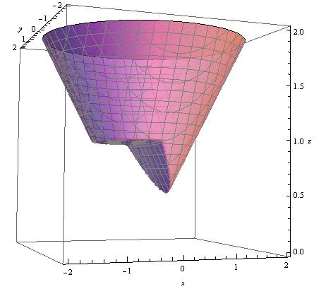
(a) $C_{1}\cup C_{2}$

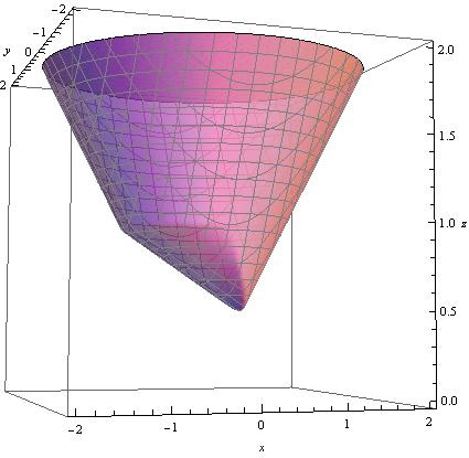
(b) $\operatorname{\overline{conv}}(C_{1}\cup C_{2})$

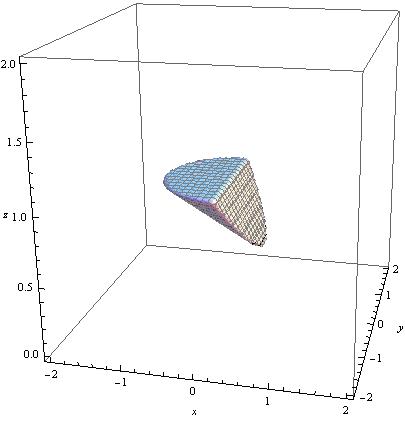
(c) $\operatorname{\overline{conv}}(C_{1}\cup C_{2})\setminus(C_{1}\cup C_{2})$

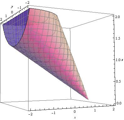
(d) Underlying cone generating the convex inequality

Figure 1: Sets associated with the disjunction $x_{3}\geq 1\,\vee\,x_{1}+x_{3}\geq 1$ on $\mathbb{K}_{2}^{3}$.

5 When are Multiple Convex Inequalities Needed?

Lemma 4 allows us to simplify the characterization (6) of undominated valid linear inequalities which are tight on both $C_{1}$ and $C_{2}$ in the case $c_{1,0}=c_{2,0}\in\{\pm 1\}$. The next proposition shows the necessity of this assumption on $c_{1,0}$ and $c_{2,0}$. Unfortunately, when $c_{1,0}\neq c_{2,0}$, undominated valid linear inequalities are tight on exactly one of the two sets $C_{1}$ and $C_{2}$. The proof of this result is left to the appendix.

Proposition 6.

Let $C_{1},C_{2}$ satisfy the basic disjunctive setup. If $c_{1,0}>c_{2,0}$, then every undominated valid linear inequality for $\operatorname{\overline{conv}}(C_{1}\cup C_{2})$ is tight on $C_{2}$ but not on $C_{1}$.

This result, when combined with Proposition 4, yields the following corollary.

Corollary 2.

Let $C_{1},C_{2}$ satisfy the basic disjunctive setup with $c_{1,0}>c_{2,0}$. If $\operatorname{\overline{conv}}(C_{1}\cup C_{2})\neq\mathbb{K}$, then $\operatorname{conv}(C_{1}\cup C_{2})$ is not closed.

Proof.

Suppose $\operatorname{conv}(C_{1}\cup C_{2})$ is closed, and let $x\in\mathbb{K}\setminus\operatorname{conv}(C_{1}\cup C_{2})$. By Proposition 4, there exists an undominated valid linear inequality which cuts off $x$ from $\operatorname{conv}(C_{1}\cup C_{2})$ and is tight on both $C_{1}$ and $C_{2}$. This contradicts Proposition 6.∎

5.1 Describing the Closed Convex Hull

As Proposition 6 hints, there are cases where valid linear inequalities that have $\beta_{1}=\beta_{2}=1$ in (6) may not be sufficient to describe $\operatorname{\overline{conv}}(C_{1}\cup C_{2})$. In this section, we study these cases when $\mathbb{K}=\mathbb{K}_{2}^{n}$ and outline a procedure to find closed-form expressions describing $\operatorname{\overline{conv}}(C_{1}\cup C_{2})$. Note that, by Theorem 2, when $c_{1}\in\mathbb{K}_{2}^{n}$ or $c_{2}\in\mathbb{K}_{2}^{n}$, the convex valid inequality (16) is sufficient to describe $\operatorname{\overline{conv}}(C_{1}\cup C_{2})$. Similarly, when the sets $D_{1}$ and $D_{2}$ defined in (LABEL:eq:BetaSets) are both nonempty, (16) is sufficient to describe $\operatorname{\overline{conv}}(C_{1}\cup C_{2})$. Hence, these cases are not of interest to us in this section, and we assume that $c_{1},c_{2}\notin\mathbb{K}_{2}^{n}$ and at least one of $D_{1}$ and $D_{2}$ is empty. We analyze the remaining cases through a breakdown based on whether $D_{1}$ and $D_{2}$ are empty or not. Note that for now we do not make the assumption that $c_{1,0}\geq c_{2,0}$; therefore, the roles of $C_{1}$ and $C_{2}$ are completely symmetric.

Let $C_{1}$ and $C_{2}$ be defined as in (2) with $\mathbb{K}=\mathbb{K}_{2}^{n}$, and let

$$B_{1}:=B_{1}(c_{1},c_{2})=\{\beta_{1}\in\mathbb{R}_{+}:\;\beta_{1}c_{1,0}\geq c_{2,0},\;c_{2}-\beta_{1}c_{1}\not\in\pm\operatorname{int}\mathbb{K}_{2}^{n}\},$$

$$B_{2}:=B_{2}(c_{1},c_{2})=\{\beta_{2}\in\mathbb{R}_{+}:\;\beta_{2}c_{2,0}\geq c_{1,0},\;c_{1}-\beta_{2}c_{2}\not\in\pm\operatorname{int}\mathbb{K}_{2}^{n}\}.$$

Using Remark Remark, it is clear that one only needs to consider $\beta_{1}\in B_{1}$ in order to capture all undominated valid linear inequalities that have a representation with $\beta_{2}=1$ in (6). Similarly, one only needs to consider $\beta_{2}\in B_{2}$ to capture the inequalities that have a representation with $\beta_{1}=1$ in (6). Therefore, by Theorem 1,

$$\operatorname{\overline{conv}}(C_{1}\cup C_{2})=\{x\in\mathbb{K}_{2}^{n}:x\text{ satisfies }\eqref{eq:main}\;\forall\beta\in B_{1}\text{ and }\eqref{eq:main2}\;\forall\beta\in B_{2}\}.$$

Note that for any $\beta_{1}\in B_{1}$ and $\beta_{2}\in B_{2}$, we have $\mathcal{N}_{1}(\beta_{1})\geq 0$ and $\mathcal{N}_{2}(\beta_{2})\geq 0$; hence, the right hand sides of the inequalities above are well defined for any $x\in\mathbb{K}_{2}^{n}$. Using the structure of $\mathbb{K}_{2}^{n}$, we can process the definition of $B_{1}$ above and arrive at

$$\!\!\!\!\!B_{1}\!\! =\!\!\{\beta\in\mathbb{R}_{+}:\;\beta c_{1,0}\geq c_{2,0},\;\left\|\tilde{c}_{2}-\beta\tilde{c_{1}}\right\|_{2}\geq|c_{2,n}-\beta c_{1,n}|\}$$

$$=\!\left\{\beta\in\mathbb{R}_{+}\!:\begin{array}[]{l}\beta c_{1,0}\geq c_{2,0},\\ \!\left(\|\tilde{c}_{1}\|_{2}^{2}\!-\!c_{1,n}^{2}\right)\beta^{2}\!-\!2\left(\tilde{c}_{1}^{\top}\tilde{c}_{2}\!-\!c_{1,n}c_{2,n}\right)\beta\!+\!\|\tilde{c}_{2}\|_{2}^{2}\!-\!c_{2,n}^{2}\!\geq 0\end{array}\right\}.$$ (21)

Similarly,

$$B_{2}\!\!=\!\!\left\{\beta\in\mathbb{R}_{+}\!:\begin{array}[]{l}\beta c_{2,0}\geq c_{1,0},\\ \!\left(\|\tilde{c}_{2}\|_{2}^{2}\!-\!c_{2,n}^{2}\right)\beta^{2}\!-\!2\left(\tilde{c}_{1}^{\top}\tilde{c}_{2}\!-\!c_{1,n}c_{2,n}\right)\beta\!+\!\|\tilde{c}_{1}\|_{2}^{2}\!-\!c_{1,n}^{2}\!\geq 0\end{array}\right\}.$$

In the following, based on the feasibility status of $D_{1},D_{2}$, we show that the description of $B_{1}$ and $B_{2}$ can be simplified.

5.1.1 $D_{1}=\emptyset$ and $D_{2}\neq\emptyset$

First note that having $D_{1}=\emptyset$ implies $c_{1}\notin-\operatorname{int}\mathbb{K}_{2}^{n}$. Furthermore, any $\beta\in D_{2}$ must satisfy $\beta>0$ since otherwise, either $c_{1}\in\mathbb{K}_{2}^{n}$ or $D_{1}\neq\emptyset$. Then by Lemma 2, $\beta c_{2,0}<c_{1,0}$, and $c_{2,0}\leq c_{1,0}$ because $\beta>0$ and $c_{1,0},c_{2,0}\in\{0,\pm 1\}$. This also implies that we cannot have $D_{1}=\emptyset$ and $D_{2}\neq\emptyset$ when $c_{1,0}=c_{2,0}=0$.

Recall that when $c_{1,0}>c_{2,0}$, Remark Remark showed that we can assume $\beta_{2}=1$ in an undominated valid linear inequality that satisfies (6). In Proposition 7 below, we prove a similar result for the case $c_{1,0}=c_{2,0}\in\{\pm 1\}$ when $D_{1}=\emptyset$ and $D_{2}\neq\emptyset$. Its proof is left to the appendix.

Proposition 7.

Let $C_{1},C_{2}$ satisfy the basic disjunctive setup with $c_{1,0}=c_{2,0}\in\{\pm 1\}$. If $D_{1}=\emptyset$ and $D_{2}\neq\emptyset$, then every undominated valid linear inequality for $\operatorname{\overline{conv}}(C_{1}\cup C_{2})$ has the form $\mu^{\top}x\geq c_{2,0}$ where $\mu$ satisfies (6) with $\beta_{2}=1$.

As a result of Proposition 7, we have

$$\operatorname{\overline{conv}}(C_{1}\cup C_{2})=\{x\in\mathbb{K}_{2}^{n}:x\text{ satisfies }\eqref{eq:main}\;\forall\beta\in B_{1}\}.$$

When $c_{1}\in-\operatorname{bd}\mathbb{K}_{2}^{n}$, we have $\|\tilde{c}_{1}\|_{2}^{2}-c_{1,n}^{2}=0$ and the second constraint in the definition of $B_{1}$ reduces to a linear inequality. Thus, $B_{1}$ is a closed interval of the nonnegative half-line in this case. On the other hand, when $c_{1}\notin\pm\mathbb{K}_{2}^{n}$, the structure of $B_{1}$ can be slightly more complicated. Since $c_{1}\notin\pm\mathbb{K}_{2}^{n}$, we can write $B_{1}$ as

$$B_{1}\!=\!\{\beta\in\mathbb{R}_{+}:\;\beta c_{1,0}\geq c_{2,0}\}\!\bigcap\left(\{\beta\!:\beta\leq\beta_{1}^{-}\}\cup\{\beta\!:\beta\geq\beta_{1}^{+}\}\right).$$

where $\beta_{1}^{\pm}$ are the values of $\beta$ that satisfy the second constraint in (21) with equality:

$$\beta_{1}^{\pm}=\frac{\tilde{c}_{1}^{\top}\tilde{c}_{2}-c_{1,n}c_{2,n}\pm\sqrt{\left(\tilde{c}_{1}^{\top}\tilde{c}_{2}-c_{1,n}c_{2,n}\right)^{2}-\left(\|\tilde{c}_{1}\|_{2}^{2}-c_{1,n}^{2}\right)\left(\|\tilde{c}_{2}\|_{2}^{2}-c_{2,n}^{2}\right)}}{\|\tilde{c}_{1}\|_{2}^{2}-c_{1,n}^{2}}.$$

Recall that any $\beta\in D_{2}$ satisfies $\beta>0$ because $c_{1}\notin\mathbb{K}_{2}^{n}$ and $D_{1}=\emptyset$. Hence, $c_{2}-\frac{1}{\beta}c_{1}\in-\mathbb{K}^{*}$, and because $c_{1}\notin\pm\mathbb{K}^{*}$, the roots $\beta_{1}^{\pm}$ are well-defined: They are exactly the values of $\beta$ that yield $c_{2}-\beta c_{1}\in-\operatorname{bd}\mathbb{K}^{*}$. Suppose $\beta_{1}^{-},\beta_{1}^{+}\in\{\beta\in\mathbb{R}_{+}:\beta c_{1,0}\geq c_{2,0}\}$. When $c_{2,0}\geq 0$, the inequality $\beta_{1}^{-}c_{1}^{\top}x\geq c_{2,0}$ dominates (or is equivalent to) all valid linear inequalities that correspond to $\beta\geq\beta^{+}$. Similarly, when $c_{2,0}=-1$, the inequality $\beta_{1}^{+}c_{1}^{\top}x\geq c_{2,0}$ dominates (or is equivalent to) all valid linear inequalities that correspond to $\beta\leq\beta^{-}$. Therefore, $B_{1}$ can always be reduced to a single closed interval of the nonnegative half-line in this case as well.

5.1.2 $D_{1}=D_{2}=\emptyset$

The hypothesis $D_{1}=D_{2}=\emptyset$ implies $c_{1},c_{2}\notin-\operatorname{int}\mathbb{K}_{2}^{n}$. Observe that for any $\beta\geq 0$, we must have $c_{2}-\beta_{1}c_{1}\notin\pm\operatorname{int}\mathbb{K}_{2}^{n}$ since having $c_{2}-\beta c_{1}\in\operatorname{int}\mathbb{K}_{2}^{n}$ contradicts $D_{1}=\emptyset$ and having $c_{2}-\beta c_{1}\in-\operatorname{int}\mathbb{K}_{2}^{n}$ contradicts $D_{2}=\emptyset$. Similarly, for any $\beta\geq 0$, we must have $c_{1}-\beta c_{2}\notin\pm\operatorname{int}\mathbb{K}_{2}^{n}$. Therefore, we can drop the second constraint in the definitions of $B_{1}$ and $B_{2}$ and write

$$B_{1}=\{\beta\in\mathbb{R}_{+}:\;\beta c_{1,0}\geq c_{2,0}\}, B_{2}=\{\beta\in\mathbb{R}_{+}:\;\beta c_{2,0}\geq c_{1,0}\}.$$

5.1.3 Finding the Best $\beta$

Suppose $C_{1}$ and $C_{2}$ satisfy the second-order disjunctive setup. For ease of notation, let us define

$$\mathcal{R}:=\mathcal{R}(c_{1},c_{2},x) =(c_{1}^{\top}x)^{2}+(\|\tilde{c}_{1}\|_{2}^{2}-c_{1,n}^{2})(x_{n}^{2}-\|\tilde{x}\|_{2}^{2}),$$

$$\mathcal{P}:=\mathcal{P}(c_{1},c_{2},x) =(c_{1}^{\top}x)(c_{2}^{\top}x)+(\tilde{c}_{1}^{\top}\tilde{c}_{2}-c_{1,n}c_{2,n})(x_{n}^{2}-\|\tilde{x}\|_{2}^{2}),$$

$$\mathcal{Q}:=\mathcal{Q}(c_{1},c_{2},x) =(c_{2}^{\top}x)^{2}+(\|\tilde{c}_{2}\|_{2}^{2}-c_{2,n}^{2})(x_{n}^{2}-\|\tilde{x}\|_{2}^{2}),$$

and $f_{1}^{c_{1},c_{2},x}(\beta):=\beta c_{1}^{\top}x+\sqrt{\mathcal{R}\beta^{2}-2\mathcal{P}\beta+\mathcal{Q}}$. Then

$$\mathcal{R}\beta^{2}-2\mathcal{P}\beta+\mathcal{Q}=\left((\beta c_{1}-c_{2})^{\top}x\right)^{2}\!+\mathcal{N}_{1}(\beta)\left(x_{n}^{2}-\|\tilde{x}\|_{2}^{2}\right).$$

Similarly, define $f_{2}^{c_{1},c_{2},x}(\beta):=\beta c_{2}^{\top}x+\sqrt{\mathcal{Q}\beta^{2}-2\mathcal{P}\beta+\mathcal{R}}$ and note

$$\mathcal{Q}\beta^{2}-2\mathcal{P}\beta+\mathcal{R}=\left((c_{1}-\beta c_{2})^{\top}x\right)^{2}\!+\mathcal{N}_{2}(\beta)\left(x_{n}^{2}-\|\tilde{x}\|_{2}^{2}\right).$$

Through these definitions, we reach

$$\operatorname{\overline{conv}}(C_{1}\cup C_{2}) =\left\{x\in\mathbb{K}_{2}^{n}:\begin{array}[]{c}2c_{2,0}-c_{2}^{\top}x\leq f_{1}^{c_{1},c_{2},x}(\beta_{1})\;~{}\forall\beta_{1}\in B_{1},\\ 2c_{2,0}-c_{1}^{\top}x\leq f_{2}^{c_{1},c_{2},x}(\beta_{2})\;~{}\forall\beta_{2}\in B_{2}\end{array}\right\}$$

$$=\left\{x\in\mathbb{K}_{2}^{n}:\begin{array}[]{c}2c_{2,0}-c_{2}^{\top}x\leq\inf_{\beta_{1}\in B_{1}}f_{1}^{c_{1},c_{2},x}(\beta_{1}),\\ 2c_{2,0}-c_{1}^{\top}x\leq\inf_{\beta_{2}\in B_{2}}f_{2}^{c_{1},c_{2},x}(\beta_{2})\end{array}\right\}.$$

For any $x\in\operatorname{bd}\mathbb{K}$, we have

$$f_{1}^{c_{1},c_{2},x}(\beta_{1})=\max\{(2\beta_{1}c_{1}-c_{2})^{\top}x,c_{2}^{\top}x\},f_{2}^{c_{1},c_{2},x}(\beta_{2})=\max\{(2\beta_{2}c_{2}-c_{1})^{\top}x,c_{1}^{\top}x\}$$

which can be easily minimized over $\beta_{1}\in B_{1}$ and $\beta_{2}\in B_{2}$. For any $x\in\operatorname{int}K$, the expressions inside the square roots in the definitions of $f_{1}^{c_{1},c_{2},x}$ and $f_{2}^{c_{1},c_{2},x}$ are strictly positive for all $\beta_{1}\in B_{1}$ and $\beta_{2}\in B_{2}$, respectively. A function of the form $g(\beta)=a\beta+\sqrt{r\beta^{2}-2p\beta+q}$ is differentiable in $\beta$ where $r\beta^{2}-2p\beta+q>0$. Furthermore, it is concave if $p^{2}\geq qr$ and convex if $p^{2}\leq qr$. Whenever the infimum of $g$ over a closed interval of the real line is finite, it will be achieved either at a critical point of $g(\beta)$, where its derivative with respect to $\beta$ vanishes, or at one of the boundary points of $B(c_{1},c_{2})$. When $r>a^{2}$ and $g$ is convex, the critical point of $g$ is given by

$$\beta^{*}=\frac{p}{r}-\frac{a}{r}\sqrt{\frac{p^{2}-qr}{a^{2}-r}},$$

and the corresponding value of the function at this critical point is

$$g(\beta^{*}) =\frac{ap}{r}+\left(1-\frac{a^{2}}{r}\right)\sqrt{\frac{p^{2}-qr}{a^{2}-r}}$$

$$=\frac{1}{r}\left(ap+\operatorname{sign}(r-a^{2})\sqrt{|(p^{2}-qr)(a^{2}-r)|}\right).$$

Replacing $p,q,r,a$ with $\mathcal{P},\mathcal{Q},\mathcal{R},c_{1}^{\top}x$, we define

$$\beta_{1}^{*}:=\beta_{1}^{*}(c_{1},c_{2},x)\!=\!\frac{\mathcal{P}}{\mathcal{R}}-\frac{c_{1}^{\top}\!x}{\mathcal{R}}\sqrt{\frac{\mathcal{P}^{2}\!-\!\mathcal{Q}\mathcal{R}}{\left(c_{1,n}^{2}\!-\!\|\tilde{c}_{1}\|_{2}^{2}\right)\left(x_{n}^{2}\!-\!\|\tilde{x}\|_{2}^{2}\right)}}.$$

Note that $c_{1,n}^{2}-\left\|\tilde{c}_{1}\right\|_{2}^{2}>0$ when $c_{1}\notin\pm\mathbb{K}^{*}$. Under these circumstances, for all $x\in\operatorname{int}\mathbb{K}_{2}^{n}$ such that $\beta_{1}^{*}(c_{1},c_{2},x)\in B_{1}(c_{1},c_{2})$, we can enforce the inequality $2c_{2,0}-c_{2}^{\top}x\leq f_{1}^{c_{1},c_{2},x}(\beta_{1}^{*})$. This inequality is only valid for those $x\in\mathbb{K}_{2}^{n}$ satisfying $\beta_{1}^{*}(c_{1},c_{2},x)\in B_{1}(c_{1},c_{2})$, but for these points, it completely summarizes all other valid inequalities of the form (8) arising from $\beta\in B_{1}(c_{1},c_{2})$.

Similarly, we define

$$\beta_{2}^{*}:=\beta_{2}^{*}(c_{1},c_{2},x)\!=\!\frac{\mathcal{P}}{\mathcal{Q}}-\frac{c_{2}^{\top}\!x}{\mathcal{Q}}\sqrt{\frac{\mathcal{P}^{2}\!-\!\mathcal{Q}\mathcal{R}}{\left(c_{2,n}^{2}\!-\!\|\tilde{c}_{2}\|_{2}^{2}\right)\left(x_{n}^{2}\!-\!\|\tilde{x}\|_{2}^{2}\right)}}.$$

Therefore, for all $x\in\operatorname{int}\mathbb{K}_{2}^{n}$ such that $\beta_{2}^{*}(c_{1},c_{2},x)\in B_{2}(c_{1},c_{2})$, we have $2c_{2,0}-c_{1}^{\top}x\leq f_{2}^{c_{1},c_{2},x}(\beta_{2}^{*})$ as a valid inequality completely summarizing all other valid inequalities of the form (12) arising from $\beta\in B_{2}(c_{1},c_{2})$.

5.2 Example where Multiple Inequalities are Needed

Consider $\mathbb{K}_{2}^{3}$ and the disjunction given by $-x_{2}\geq 0$ or $-x_{3}\geq-1$. Since $c_{1,0}>c_{2,0}$, by Proposition 6, we know that every undominated valid linear inequality for $\operatorname{\overline{conv}}(C_{1}\cup C_{2})$ will be tight on $C_{2}$ but not on $C_{1}$. Therefore, we follow the approach outlined in Section 5.1. By noting that $c_{1}=-e^{2}\not\in\pm K_{2}^{3}$, we obtain $B_{1}(c_{1},c_{2})=\{\beta\in\mathbb{R}:\,\beta\geq 1\}$. It is also clear that $B_{2}(c_{1},c_{2})=\emptyset$ in this case.

In this setup we have

$$\mathcal{R}(c_{1},c_{2},x) =x_{3}^{2}-x_{1}^{2},$$

$$\mathcal{P}(c_{1},c_{2},x) =x_{2}x_{3},$$

$$\mathcal{Q}(c_{1},c_{2},x) =x_{1}^{2}+x_{2}^{2},$$

and the resulting $f_{1}^{c_{1},c_{2},x}(\beta)$ is a convex function of $\beta$. Hence we get

$$\beta_{1}^{*}(c_{1},c_{2},x) =\frac{x_{2}x_{3}}{x_{3}^{2}-x_{1}^{2}}+\frac{x_{2}}{x_{3}^{2}-x_{1}^{2}}\sqrt{\frac{x_{2}^{2}x_{3}^{2}-(x_{1}^{2}+x_{2}^{2})(x_{3}^{2}-x_{1}^{2})}{(-1)(x_{3}^{2}-x_{1}^{2}-x_{2}^{2})}}$$

$$=\frac{x_{2}x_{3}+|x_{1}|x_{2}}{x_{3}^{2}-x_{1}^{2}}=\frac{x_{2}}{x_{3}-|x_{1}|}$$

where in the last equation we used the fact that $x\in\mathbb{K}_{2}^{3}$ and hence $x_{3}\geq 0$. This leads to $f_{1}^{c_{1},c_{2},x}(\beta_{1}^{*})=|x_{1}|-\frac{x_{2}^{2}(x_{3}+|x_{1}|)}{x_{3}^{2}-x_{1}^{2}}=|x_{1}|-\frac{x_{2}^{2}}{x_{3}-|x_{1}|}$.

Therefore, for all $x\in\mathbb{K}_{2}^{3}$ such that $\beta_{1}^{*}\geq 1$, that is, $|x_{1}|\geq x_{3}-x_{2}$, we can enforce $2c_{2,0}-c_{2}^{\top}x\leq f_{1}^{c_{1},c_{2},x}(\beta_{1}^{*})$ which translates to $-2+x_{3}\leq|x_{1}|-\frac{x_{2}^{2}}{x_{3}-|x_{1}|}$ in this example. Moreover, $\operatorname{bd}B_{1}(c_{1},c_{2})=\{1\}$, and for this particular value of $\beta=1$, using (7) in Remark Remark, we obtain $x_{2}\leq 1$ as a valid linear inequality for all $x\in\operatorname{\overline{conv}}(C_{1}\cup C_{2})$. Putting these two inequalities together, we arrive at

$$\operatorname{\overline{conv}}(C_{1}\cup C_{2})=\left\{x\in\mathbb{K}_{2}^{3}\!:\;x_{2}\leq 1,\;1+|x_{1}|-x_{3}\leq\sqrt{1-\max\{0,x_{2}\}^{2}}\right\},$$

where both inequalities are convex (even when we ignore the constraint $x\in\mathbb{K}_{2}^{3}$). In fact, both inequalities describing $\operatorname{\overline{conv}}(C_{1}\cup C_{2})$ are conic quadratic representable in a lifted space as expected.

In Figures 2(a) and (b), we plot the disjunctive set and the resulting closed convex hull, respectively. In order to give a better picture of the convexification of the set, we show the points added due to the convex hull operation in Figure 2(c).

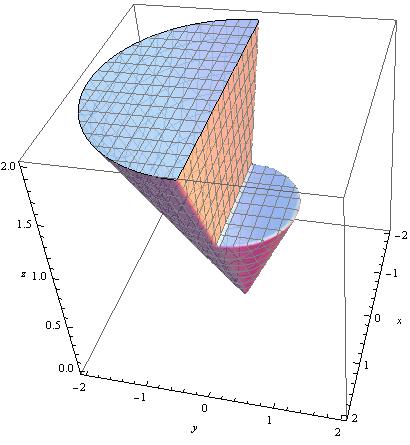
(a) $C_{1}\cup C_{2}$

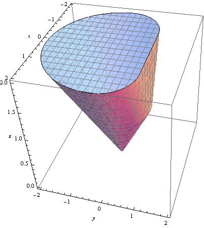
(b) $\operatorname{\overline{conv}}(C_{1}\cup C_{2})$

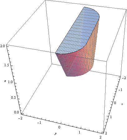
(c) $\operatorname{\overline{conv}}(C_{1}\cup C_{2})\setminus(C_{1}\cup C_{2})$

Figure 2: Sets associated with the disjunction $-x_{2}\geq 0\,\vee\,-x_{3}\geq-1$ on $\mathbb{K}_{2}^{3}$.

6 Elementary Split Disjunctions for $p$-order Cones

Given $w\in\mathbb{R}^{d}$ and $p\in(1,\infty)$, recall that the $p$-norm $\left\|\cdot\right\|_{p}:\mathbb{R}^{d}\rightarrow\mathbb{R}$ is defined as

$$\left\|w\right\|_{p}:=\left(\sum_{j=1}^{d}|w_{j}|^{p}\right)^{1/p}.$$

Its dual norm is the function $\left\|\xi\right\|_{p}^{*}:=\max\{\xi^{\top}w:\,\left\|w\right\|_{p}\leq 1\,\forall w\in\mathbb{R}^{d}\}$ and corresponds to the $q$-norm on $\mathbb{R}^{d}$ where $\frac{1}{p}+\frac{1}{q}=1$. In this section we consider the $n$-dimensional $p$-order cone $\mathbb{K}_{p}^{n}:=\left\{x\in\mathbb{R}^{n}:\left\|\tilde{x}\right\|_{p}\leq x_{n}\right\}$, which is a regular cone and whose dual cone is simply $\mathbb{K}_{q}^{n}$.

The main result of this section shows that the techniques of the previous sections can be used to describe the convex hull of the set obtained by applying an elementary split disjunction on $\mathbb{K}_{p}^{n}$. Let $c_{1}=t_{1}e^{i}$, $c_{2}=-t_{2}e^{i}$, $c_{1,0},c_{2,0}\in\{0,\pm 1\}$ where $t_{1},t_{2}>0$, $e^{i}$ is the $i^{\text{th}}$ standard unit vector, and $i\in\{1,\ldots,n-1\}$. Note that $\operatorname{conv}(C_{1}\cup C_{2})$ is closed by Corollary 1 and $\operatorname{conv}(C_{1}\cup C_{2})=\mathbb{K}_{p}^{n}$ unless $c_{1,0}=c_{2,0}=1$ by Lemma 1. Hence, we consider the case $c_{1,0}=c_{2,0}=1$ only. This result recovers and provides an independent proof of Corollary 1 in [26]. Its proof follows the same outline as the proof of Theorem 1 and is therefore left to the appendix.

Corollary 3.

Let $C_{1}:=\{x\in\mathbb{K}_{p}^{n}:\,t_{1}x_{i}\geq 1\}$ and $C_{2}:=\{x\in\mathbb{K}_{p}^{n}:\;-t_{2}x_{i}\geq 1\}$ where $t_{1},t_{2}>0$, $p\in(1,\infty)$, and $i\in\{1,\ldots,n-1\}$. Let $e^{i}$ denote the $i^{\text{th}}$ standard unit vector. Then

$$\operatorname{conv}(C_{1}\cup C_{2})=\left\{x\in\mathbb{K}_{p}^{n}:\;\left\|(t_{1}+t_{2})\tilde{x}-2(t_{2}x_{i}+1)\tilde{e}^{i}\right\|_{p}\leq(t_{1}+t_{2})x_{n}\right\}.$$

7 Appendix

7.1 Proofs of Section 2

of Lemma 1.

To prove the first claim, suppose $S_{1}\cup S_{2}\subsetneq S$ and pick $x_{0}\in S\setminus(S_{1}\cup S_{2})$. Also, pick $x_{1}\in S_{1}\setminus S_{2}$ and $x_{2}\in S_{2}\setminus S_{1}$. Let $x^{\prime}$ be the point on the line segment between $x_{0}$ and $x_{1}$ such that $c_{1}^{\top}x^{\prime}=c_{1,0}$. Similarly, let $x^{\prime\prime}$ be the point between $x_{0}$ and $x_{2}$ such that $c_{2}^{\top}x^{\prime\prime}=c_{2,0}$. Note that $x^{\prime}\notin S_{2}$ and $x^{\prime\prime}\notin S_{1}$ by the convexity of $S\setminus S_{1}$ and $S\setminus S_{2}$. Then a point that is a strict convex combination of $x^{\prime}$ and $x^{\prime\prime}$ is in $\operatorname{conv}(S_{1}\cup S_{2})$ but not in $S_{1}\cup S_{2}$.

Corollary 9.1.2 in [28] implies $S_{1}^{+}$ and $S_{2}^{+}$ are closed and $\operatorname{rec}S_{1}^{+}=\operatorname{rec}S_{2}^{+}=\operatorname{rec}S_{1}+\operatorname{rec}S_{2}$ because $S$ is pointed. The inclusions $S_{1}\subseteq S_{1}^{+}$ and $S_{2}\subseteq S_{2}^{+}$ imply that $\operatorname{conv}(S_{1}\cup S_{2})\subseteq\operatorname{conv}(S_{1}^{+}\cup S_{2}^{+})$. Furthermore, $\operatorname{conv}(S_{1}^{+}\cup S_{2}^{+})$ is closed by Corollary 9.8.1 in [28] since $S_{1}^{+}$ and $S_{2}^{+}$ have the same recession cone. Hence, $\operatorname{\overline{conv}}(S_{1}\cup S_{2})\subseteq\operatorname{conv}(S_{1}^{+}\cup S_{2}^{+})$. We claim $\operatorname{\overline{conv}}(S_{1}\cup S_{2})=\operatorname{conv}(S_{1}^{+}\cup S_{2}^{+})$. Let $x^{+}\in\operatorname{conv}(S_{1}^{+}\cup S_{2}^{+})$. Then there exist $u_{1}\in S_{1}$, $v_{2}\in\operatorname{rec}S_{2}$, $u_{2}\in S_{2}$, and $v_{1}\in\operatorname{rec}S_{1}$ such that $x^{+}\in\operatorname{conv}\{u_{1}+v_{2},u_{2}+v_{1}\}$. To prove the claim, it is enough to show that $u_{1}+v_{2},u_{2}+v_{1}\in\operatorname{\overline{conv}}(S_{1}\cup S_{2})$. Consider the point $u_{1}+v_{2}$ and the sequence

$$\left\{\left(1-\frac{1}{k}\right)u_{1}+\frac{1}{k}\left(u_{2}+kv_{2}\right)\right\}_{k\in\mathbb{N}}.$$

For any $k\in\mathbb{N}$, we have $u_{1}\in S_{1}$ and $u_{2}+kv_{2}\in S_{2}$. Therefore, this sequence is in $\operatorname{conv}(S_{1}\cup S_{2})$. Furthermore, it converges to $u_{1}+v_{2}$ as $k\rightarrow\infty$ which implies $u_{1}+v_{2}\in\operatorname{\overline{conv}}(S_{1}\cup S_{2})$. A similar argument shows $u_{2}+v_{1}\in\operatorname{\overline{conv}}(S_{1}\cup S_{2})$ and proves the claim.∎

7.2 Proofs of Section 4

of Proposition 5.

Let $S_{1}^{+}:=S_{1}+\operatorname{rec}S_{2}$ and $S_{2}^{+}:=S_{2}+\operatorname{rec}S_{1}$. We have $\operatorname{conv}(S_{1}\cup S_{2})\subseteq\operatorname{\overline{conv}}(S_{1}\cup S_{2})=\operatorname{conv}(S_{1}^{+}\cup S_{2}^{+})$ by Lemma 1. We are going to show $\operatorname{conv}(S_{1}^{+}\cup S_{2}^{+})\subseteq\operatorname{conv}(S_{1}\cup S_{2})$ to prove that $\operatorname{conv}(S_{1}\cup S_{2})$ is closed when (LABEL:eq:ClosedSuff) is satisfied. Let $x^{+}\in S_{1}^{+}$. Then there exist $u_{1}\in S_{1}$ and $v_{2}\in\operatorname{rec}(S_{2})$ such that $x^{+}=u_{1}+v_{2}$. If $c_{2}^{\top}v_{2}>0$, then there exists $\epsilon\geq 1$ such that $x^{+}+\epsilon v_{2}\in S_{2}$ and we have $x^{+}\in\operatorname{conv}(S_{1}\cup S_{2})$. Otherwise, $c_{2}^{\top}v_{2}=0$, and by the hypothesis, $c_{1}^{\top}v_{2}\geq 0$. This implies $x^{+}\in S_{1}$, and thus $S_{1}^{+}\subseteq\operatorname{conv}(S_{1}\cup S_{2})$. Through a similar argument, one can show $S_{2}^{+}\subseteq\operatorname{conv}(S_{1}\cup S_{2})$. Hence, $S_{1}^{+}\cup S_{2}^{+}\subseteq\operatorname{conv}(S_{1}\cup S_{2})$. Taking the convex hull of both sides yields $\operatorname{conv}(S_{1}^{+}\cup S_{2}^{+})\subseteq\operatorname{conv}(S_{1}\cup S_{2})$.

For the converse, suppose condition (i) holds, and let $x^{*}\in S_{1}$ be such that $c_{2}^{\top}x^{*}\leq c_{2}^{\top}x$ for all $x\in S_{1}$. Note that $c_{2}^{\top}x^{*}<c_{2,0}$ since otherwise, $S_{1}\subseteq S_{2}$. Pick $\delta>0$ such that $x^{\prime}:=x^{*}+\delta r^{*}\notin S_{1}$. Then $x^{\prime}\notin S_{2}$ too because $c_{2}^{\top}x^{\prime}=c_{2}^{\top}x^{*}<c_{2,0}$. For any $0<\lambda<1$, $x_{1}\in S_{1}$, and $x_{2}\in S_{2}$, we can write $c_{2}^{\top}(\lambda x_{1}+(1-\lambda)x_{2})\geq\lambda c_{2}^{\top}x^{*}+(1-\lambda)c_{2,0}>c_{2}^{\top}x^{\prime}$. Hence, $x^{\prime}\notin\operatorname{conv}(S_{1}\cup S_{2})$. On the other hand, $x^{\prime}\in S_{1}^{+}\subseteq\operatorname{conv}(S_{1}^{+}\cup S_{2}^{+})=\operatorname{\overline{conv}}(S_{1}\cup S_{2})$ where the last equality follows from Lemma 1.∎

of Corollary 1.

Suppose there exist $\beta_{1},\beta_{2}\in\mathbb{R}$ such that $c_{1}-\beta_{2}c_{2}\in\mathbb{K}^{*}$ and $c_{2}-\beta_{1}c_{1}\in\mathbb{K}^{*}$. Consider the following minimization problem

$$\inf_{u}\{c_{1}^{\top}u:\;c_{2}^{\top}u=0,u\in\mathbb{K}\}$$

and its dual

$$\sup_{\delta}\{0:\;c_{1}-\delta c_{2}\in\mathbb{K}^{*}\}.$$

Because $\beta_{2}$ is a feasible solution to the dual problem, we have $c_{1}^{\top}u\geq 0$ for all $u\in\mathbb{K}$ such that $c_{2}^{\top}u=0$. Similarly, one can use the existence of $\beta_{1}$ to show that the second part of (LABEL:eq:ClosedSuff) holds too. Then by Proposition 5, $\operatorname{conv}(C_{1}\cup C_{2})$ is closed.∎

7.3 Proofs of Section 5

of Proposition 6.

Every undominated valid inequality has to be tight on either $C_{1}$ or $C_{2}$; otherwise, we can just increase the right-hand side to obtain a dominating valid inequality. By Proposition 1, undominated valid inequalities are of the form $\mu^{\top}x\geq c_{2,0}$ with $(\mu,\alpha_{1},\alpha_{2},\beta_{1},\beta_{2})$ satisfying (6). In particular, we have $\beta_{1},\beta_{2}>0$ such that $\min\{\beta_{1}c_{1,0},\beta_{2}c_{2,0}\}=c_{2,0}$. Now consider the following minimization problem

$$\inf_{u}\{\mu^{\top}u:\;u\in C_{1}\}$$

and its dual

$$\sup_{\delta}\{\delta c_{1,0}:\;\mu-\delta c_{1}\in\mathbb{K}^{*},\;\delta\geq 0\}.$$

$C_{1}$ is a strictly feasible set by Assumption 2, so strong duality applies to this pair of problems and the dual problem admits an optimal solution $\delta^{*}\geq\beta_{1}>0$. Then

$$\operatorname{sign}\{\delta^{*}c_{1,0}\}=\operatorname{sign}\{c_{1,0}\}=c_{1,0}>c_{2,0}.$$

Hence, the inequality $\mu^{\top}x\geq\mu_{0}$ cannot be tight on $C_{1}$.∎

of Proposition 7.

Let $\nu^{\top}x\geq c_{2,0}$ be a valid inequality of the form (6). Then there exist $\alpha_{1},\alpha_{2},\beta_{1},\beta_{2}$ such that $(\nu,\alpha_{1},\alpha_{2},\beta_{1},\beta_{2})$ satisfies (6). In particular, $\min\{\beta_{1}c_{1,0},\beta_{2}c_{2,0}\}=c_{2,0}$. If $\beta_{2}c_{2,0}=c_{2,0}$, then $\beta_{2}=1$ and $\nu^{\top}x\geq c_{2,0}$ already has the desired form. Therefore, suppose $\beta_{2}c_{2,0}>c_{2,0}$. Then $c_{2,0}=\beta_{1}c_{1,0}=\beta_{1}c_{2,0}$ and thus $\beta_{1}=1$. We are going to show that $\nu^{\top}x\geq c_{2,0}$ is either dominated or has itself an equivalent representation (6) of the type claimed in the lemma.

Let $\delta\in D_{2}(c_{1},c_{2})$ and let $\gamma:=c_{1}-\delta c_{2}\in\mathbb{K}^{*}$. Then $\delta\geq 0$ because $D_{1}(c_{1},c_{2})=\emptyset$, and using Lemma 2, we have $\delta c_{2,0}<c_{1,0}=c_{2,0}$, which implies $\delta<1$. Then we can select $0<\lambda<1$ such that $\lambda\beta_{2}c_{2,0}+(1-\lambda)\delta c_{2,0}=c_{2,0}$. Let us define $\alpha_{1}^{\prime}:=\lambda\alpha_{1}$, $\alpha_{2}^{\prime}:=\lambda\alpha_{2}+(1-\lambda)\gamma$, $\beta_{2}^{\prime}:=\lambda\beta_{2}+(1-\lambda)\delta=1$, and $\mu:=\lambda\nu+(1-\lambda)c_{1}=\lambda\alpha_{1}+c_{1}$. With these definitions, $\mu^{\top}x\geq c_{2,0}$ is a valid inequality for $\operatorname{\overline{conv}}(C_{1}\cup C_{2})$ because $(\mu,c_{2,0},\alpha_{1}^{\prime},\alpha_{2}^{\prime},1,1)$ satisfies (5). Furthermore, $\nu-\mu=(1-\lambda)\alpha_{1}\in\mathbb{K}^{*}$. This shows that $\nu^{\top}x\geq c_{2,0}$ is dominated by $\mu^{\top}x\geq c_{2,0}$ if $\alpha_{1}\neq 0$ and has an equivalent representation (5) with $\beta_{2}^{\prime}=1$ if $\alpha_{1}=0$. In the first case, we are done. In the second case, we are done if $\alpha_{2}^{\prime}\in\operatorname{bd}\mathbb{K}^{*}$. Otherwise, we can find a valid inequality that dominates $\nu^{\top}x\geq 1$ as in the proof of Proposition 1.∎

7.4 Proofs of Section 6

of Corollary 3.

Let $q\in(1,\infty)$ be such that $\frac{1}{p}+\frac{1}{q}=1$. The sets $C_{1}$ and $C_{2}$ satisfy Assumptions 1 and 2 because $e^{i}\notin\mathbb{K}_{q}^{n}$. Since we are considering a split disjunction, $\operatorname{conv}(C_{1}\cup C_{2})$ is closed by Corollary 1. Using Propositions 1 and 4 and Lemma 4, we see that any undominated valid linear inequality for $\operatorname{conv}(C_{1}\cup C_{2})$ has the form $\mu^{\top}x\geq 1$ with $(\mu,\alpha_{1},\alpha_{2})$ satisfying

$$\begin{gathered}\mu=\alpha_{1}+t_{1}e^{i},\\ \mu=\alpha_{2}-t_{2}e^{i},\\ \alpha_{1},\alpha_{2}\in\operatorname{bd}\mathbb{K}_{q}^{n}.\end{gathered}$$

Let

$$M\!:=\left\{\mu\in\mathbb{R}^{n}\!:\,\exists\alpha_{1},\alpha_{2}\in\operatorname{bd}\mathbb{K}_{q}^{n}~{}\text{ s.t. }~{}\mu=\alpha_{1}+t_{1}e^{i}=\alpha_{2}-t_{2}e^{i}\right\}.$$

Then we can write

$$M= \left\{\mu\in\mathbb{R}^{n}:\;\left\|\tilde{\mu}-t_{1}\tilde{e}^{i}\right\|_{q}=\mu_{n},\;\left\|\tilde{\mu}+t_{2}\tilde{e}^{i}\right\|_{q}=\mu_{n}\right\}$$

$$= \left\{\mu\in\mathbb{R}^{n}:\;\left\|\tilde{\mu}-t_{1}\tilde{e}^{i}\right\|_{q}=\left\|\tilde{\mu}+t_{2}\tilde{e}^{i}\right\|_{q},\;\left\|\tilde{\mu}+t_{2}\tilde{e}^{i}\right\|_{q}=\mu_{n}\right\}$$

$$= \left\{\mu\in\mathbb{R}^{n}:\;2\mu_{i}=t_{1}-t_{2},\;\left\|\tilde{\mu}+t_{2}\tilde{e}^{i}\right\|_{q}=\mu_{n}\right\}.$$

Therefore, we obtain

$$x \in\operatorname{conv}(C_{1}\cup C_{2})\Leftrightarrow x\in\mathbb{K}_{p}^{n}\text{ and }\mu^{\top}x\geq 1\;~{}\forall\mu\in M.$$

$$\Leftrightarrow x\in\mathbb{K}_{2}^{n}\text{ and }\inf_{\mu}\left\{\mu^{\top}x:\;\mu\in M(\beta,1)\right\}\geq 1.$$

Note that the second equality constraint in the description of $M$ makes this optimization problem non-convex. However, we can relax this problematic constraint to an inequality without any loss of generality. In fact, consider the relaxation

$$\inf_{\mu}\left\{\mu^{\top}x:\;2\mu_{i}=t_{1}-t_{2},\;\left\|\tilde{\mu}+t_{2}\tilde{e}^{i}\right\|_{q}\leq\mu_{n}\right\}.$$

The feasible region of this relaxation is the intersection of a hyperplane with a closed, convex cone shifted by the vector $t_{2}e^{i}$. Any solution which is feasible to the relaxation but not the original problem can be expressed as a convex combination of solutions feasible to the original problem. Because we are optimizing a linear function, this shows that the relaxation is equivalent to the original problem. Thus, we have

$$x \in\operatorname{conv}(C_{1}\cup C_{2})$$

$$\Leftrightarrow x\in\mathbb{K}_{p}^{n}\text{ and }\inf_{\mu}\left\{\mu^{\top}x:\;2\mu_{i}=t_{1}-t_{2},\;\mu+t_{2}e^{i}\in\mathbb{K}_{q}^{n}\right\}\geq 1.$$

The minimization problem in the last line above is strictly feasible since $e^{n}$ is a recession direction of the feasible region and belongs to $\operatorname{int}\mathbb{K}_{q}^{n}$. Hence, its dual problem is solvable whenever it is feasible, strong duality applies, and we can replace the problem in the last line with its dual without any loss of generality. The dual problem is given by

$$\sup_{\rho,\tau}\left\{-t_{2}(e^{i})^{\top}\rho+(t_{1}-t_{2})\tau:\;\rho+2\tau e^{i}=x,\;\rho\in\mathbb{K}_{p}^{n}\right\}$$

$$= \sup_{\tau}\left\{-t_{2}x_{i}+(t_{1}+t_{2})\tau:\;x-2\tau e^{i}\in\mathbb{K}_{p}^{n}\right\}$$

and it is feasible for $x\in\mathbb{K}_{p}^{n}$ with $\tau=0$. Thus, we obtain

$$x\in \operatorname{conv}(C_{1}\cup C_{2})$$

$$\Leftrightarrow x\in\mathbb{K}_{p}^{n}\text{ and }\sup_{\tau}\left\{-t_{2}x_{i}+(t_{1}+t_{2})\tau:\;x-2\tau e^{i}\in\mathbb{K}_{p}^{n}\right\}\geq 1.$$

Note that, for any given $x\in\mathbb{K}_{p}^{n}$, the problem above involves maximizing a linear function over a closed interval and the coefficient of $\tau$ in the objective function is positive; therefore, the optimum solution $\tau^{*}(x)$ will occur at the larger of the two endpoints of this interval which is

$$\tau^{*}(x)=\frac{1}{2}x_{i}+\left(x_{n}^{p}-\sum_{j\notin\{i,n\}}|x_{j}|^{p}\right)^{\frac{1}{p}}.$$

Therefore,

$$x\in \operatorname{conv}(C_{1}\cup C_{2})$$

$$\Leftrightarrow x\in\mathbb{K}_{p}^{n}\mbox{ and }-t_{2}x_{i}+(t_{1}+t_{2})\tau^{*}(x)\geq 1.$$

$$\Leftrightarrow x\in\mathbb{K}_{p}^{n}\mbox{ and }\frac{2-(t_{1}-t_{2})x_{i}}{t_{1}+t_{2}}\leq\left(x_{n}^{p}-\sum_{j\notin\{i,n\}}|x_{j}|^{p}\right)^{\frac{1}{p}}.$$ (22)

The validity and convexity of the above inequality follow from its derivation. Moreover, due to its derivation, this inequality precisely captures all of the undominated valid linear inequalities for $C_{1}\cup C_{2}$. Hence, together with the cone constraint $x\in\mathbb{K}_{p}^{n}$, the inequality (22) is sufficient to describe $\operatorname{conv}(C_{1}\cup C_{2})$.

In order to arrive at Corollary 3, we further claim that, for all $x\in\mathbb{K}_{p}^{n}$,

$$\frac{-2+(t_{1}-t_{2})x_{i}}{t_{1}+t_{2}}\leq\left(x_{n}^{p}-\sum_{j\notin\{i,n\}}|x_{j}|^{p}\right)^{\frac{1}{p}}.$$ (23)

Let $u\in\mathbb{K}_{p}^{n}$. When $(t_{1}-t_{2})u_{i}\leq 2$, the left-hand side of (23) is non-positive and the claim is satisfied trivially. Otherwise, $(t_{1}-t_{2})u_{i}>2$ which implies that either $t_{1}u_{i}>1$ ($u\in C_{1}$) or $-t_{2}u_{i}>1$ ($u\in C_{2}$). Because $u\in\mathbb{K}_{p}^{n}$, we can write $\left(u_{n}^{p}-\sum_{j\notin\{i,n\}}|u_{j}|^{p}\right)^{\frac{1}{p}}\geq|u_{i}|$; therefore, all we need to show is that $|u_{i}|\geq\frac{(t_{1}-t_{2})u_{i}-2}{t_{1}+t_{2}}$ or, equivalently, $(t_{1}+t_{2})|u_{i}|\geq(t_{1}-t_{2})u_{i}-2$. Suppose $u\in C_{1}$. Then we have $t_{1}u_{i}\geq 1$, and since $C_{1}\cap C_{2}=\emptyset$, we get $u\not\in C_{2}$, implying $-t_{2}u_{i}<1$. Therefore, $-2+(t_{1}-t_{2})u_{i}<(2t_{2}u_{i})+(t_{1}-t_{2})u_{i}=(t_{1}+t_{2})u_{i}\leq|(t_{1}+t_{2})u_{i}|$ which proves the desired relation. Now suppose $u\in C_{2}$. Similarly, we obtain $t_{1}u_{i}<1$ which allows us to write $-2+(t_{1}-t_{2})u_{i}<-2t_{1}u_{i}+(t_{1}-t_{2})u_{i}=-(t_{1}+t_{2})u_{i}\leq|(t_{1}+t_{2})u_{i}|$ and completes the proof of the claim.

By combining the inequalities (22) and (23), we conclude that

$$\frac{|2-(t_{1}-t_{2})x_{i}|}{t_{1}+t_{2}}\leq\left(x_{n}^{p}-\sum_{j\notin\{i,n\}}|x_{j}|^{p}\right)^{\frac{1}{p}}.$$

Noting that $t_{1}+t_{2}>0$, taking the $p$-th power of both sides of the above inequality, and rearranging its terms, we arrive at

$$\left(\left|(t_{1}-t_{2})x_{i}-2\right|^{p}+(t_{1}+t_{2})^{p}\sum_{j\notin\{i,n\}}|x_{j}|^{p}\right)^{\frac{1}{p}}\leq(t_{1}+t_{2})x_{n}$$

which can be equivalently expressed as the desired conic valid inequality.∎

References

- [1] K. Andersen and A. N. Jensen. Intersection cuts for mixed integer conic quadratic sets. In Proceedings of IPCO 2013, volume 7801 of Lecture Notes in Computer Science, pages 37–48, Valparaiso, Chile, March 2013.
- [2] A. Atamtürk and V. Narayanan. Conic mixed-integer rounding cuts. Mathematical Programming, 122(1):1–20, 2010.
- [3] A. Atamtürk and V. Narayanan. Lifting for conic mixed-integer programming. Mathematical Programming, 126(2):351–363, 2011.
- [4] E. Balas. Intersection cuts - a new type of cutting planes for integer programming. Operations Research, 19:19–39, 1971.
- [5] E. Balas. Disjunctive programming: Properties of the convex hull of feasible points. GSIA Management Science Research Report MSRR 348, published as invited paper in Discrete Applied Mathematics 89 (1998), 1974.
- [6] E. Balas. Disjunctive programming. Annals of Discrete Mathematics, 5:3–51, 1979.
- [7] E. Balas, S. Ceria, and G. Cornuéjols. A lift-and-project cutting plane algorithm for mixed 0-1 programs. Mathematical Programming, 58:295–324, 1993.
- [8] P. Belotti. Disjunctive cuts for nonconvex MINLP. In Jon Lee and Sven Leyffer, editors, Mixed Integer Nonlinear Programming, volume 154 of The IMA Volumes in Mathematics and its Applications, pages 117–144. Springer, New York, NY, 2012.
- [9] P. Belotti, J. C. Goez, I. Polik, T. K. Ralphs, and T. Terlaky. A conic representation of the convex hull of disjunctive sets and conic cuts for integer second order cone optimization. Technical report, Department of Industrial and Systems Engineering, Lehigh University, Bethlehem, PA, June 2012.
- [10] P. Belotti, J.C. Góez, I. Pólik, T.K. Ralphs, and T. Terlaky. On families of quadratic surfaces having fixed intersections with two hyperplanes. Discrete Applied Mathematics, 161(16):2778–2793, 2013.
- [11] H. Y. Benson and U. Saglam. Mixed-integer second-order cone programming: A survey. Tutorials in Operations Research, pages 13–36. INFORMS, Hanover, MD, 2013.
- [12] D. Bienstock and A. Michalka. Cutting-planes for optimization of convex functions over nonconvex sets. SIAM Journal on Optimization, 24(2):643–677, 2014.
- [13] P. Bonami. Lift-and-project cuts for mixed integer convex programs. In O. Gunluk and G. J. Woeginger, editors, Proceedings of the 15th IPCO Conference, volume 6655 of Lecture Notes in Computer Science, pages 52–64, New York, NY, 2011. Springer.
- [14] P. Bonami, M. Conforti, G. Cornuéjols, M. Molinaro, and G. Zambelli. Cutting planes from two-term disjunctions. Operations Research Letters, 41:442–444, 2013.
- [15] S. Burer and A.N. Letchford. Non-convex mixed-integer nonlinear programming: A survey. Surveys in Operations Research and Management Science, 17(2):97 – 106, 2012.
- [16] S. Burer and A. Saxena. The MILP road to MIQCP. In Mixed Integer Nonlinear Programming, pages 373–405. Springer, 2012.
- [17] F. Cadoux. Computing deep facet-defining disjunctive cuts for mixed-integer programming. Mathematical Programming, 122(2):197–223, 2010.
- [18] M. Çezik and G. Iyengar. Cuts for mixed 0-1 conic programming. Mathematical Programming, 104(1):179–202, 2005.
- [19] G. Cornuéjols and C. Lemaréchal. A convex-analysis perspective on disjunctive cuts. Mathematical Programming, 106(3):567–586, 2006.
- [20] D. Dadush, S. S. Dey, and J. P. Vielma. The split closure of a strictly convex body. Operations Research Letters, 39:121–126, 2011.
- [21] S. Drewes. Mixed Integer Second Order Cone Programming. PhD thesis, Technische Universität Darmstadt, 2009.
- [22] S. Drewes and S. Pokutta. Cutting-planes for weakly-coupled 0/1 second order cone programs. Electronic Notes in Discrete Mathematics, 36:735–742, 2010.
- [23] J. J. Júdice, H. Sherali, I. M. Ribeiro, and A. M. Faustino. A complementarity-based partitioning and disjunctive cut algorithm for mathematical programming problems with equilibrium constraints. Journal of Global Optimization, 136:89–114, 2006.
- [24] M. R. Kılınç, J. Linderoth, and J. Luedtke. Effective separation of disjunctive cuts for convex mixed integer nonlinear programs. Technical report, 2010. http://www.optimization-online.org/DB_FILE/2010/11/2808.pdf.
- [25] F. Kılınç-Karzan. On minimal valid inequalities for mixed integer conic programs. GSIA Working Paper Number: 2013-E20, GSIA, Carnegie Mellon University, Pittsburgh, PA, June 2013.
- [26] S. Modaresi, M. R. Kılınç, and J. P. Vielma. Intersection cuts for nonlinear integer programming: Convexification techniques for structured sets. Working paper, March 2013.
- [27] S. Modaresi, M. R. Kılınç, and J. P. Vielma. Split cuts and extended formulations for mixed integer conic quadratic programming. Working paper, February 2014.
- [28] R. T. Rockafellar. Convex Analysis. Princeton Landmarks in Mathematics. Princeton University Press, New Jersey, 1970.
- [29] A. Saxena, P. Bonami, and J. Lee. Disjunctive cuts for non-convex mixed integer quadratically constrained programs. In A. Lodi, A. Panconesi, and G. Rinaldi, editors, IPCO, volume 5035 of Lecture Notes in Computer Science, pages 17–33. Springer, 2008.
- [30] H.D. Sherali and C. Shetti. Optimization with disjunctive constraints. Lectures on Econ. Math. Systems, 181, 1980.
- [31] R. A. Stubbs and S. Mehrotra. A branch-and-cut method for 0-1 mixed convex programming. Mathematical Programming, 86(3):515–532, 1999.
- [32] M. Tawarmalani, J.P. Richard, and K. Chung. Strong valid inequalities for orthogonal disjunctions and bilinear covering sets. Mathematical Programming, 124(1-2):481–512, 2010.