Accurate Simulation of Ideal Circular and Elliptic Cylindrical Invisibility Cloaks

Abstract.

The coordinate transformation offers a remarkable way to design cloaks that can steer electromagnetic fields so as to prevent waves from penetrating into the cloaked region (denoted by $\Omega_{0}$, where the objects inside are invisible to observers outside). The ideal circular and elliptic cylindrical cloaked regions are blown up from a point and a line segment, respectively, so the transformed material parameters and the corresponding coefficients of the resulted equations are highly singular at the cloaking boundary $\partial\Omega_{0}$. The electric field or magnetic field is not continuous across $\partial\Omega_{0}.$ The imposition of appropriate cloaking boundary conditions (CBCs) to achieve perfect concealment is a crucial but challenging issue.

Based upon the principle that finite electromagnetic fields in the original space must be finite in the transformed space as well, we obtain CBCs that intrinsically relate to the essential “pole” conditions of a singular transformation. We also find that for the elliptic cylindrical cloak, the CBCs should be imposed differently for the cosine-elliptic and sine-elliptic components of the decomposed fields. With these at our disposal, we can rigorously show that the governing equation in $\Omega_{0}$ can be decoupled from the exterior region $\Omega_{0}^{c}$, and the total fields in the cloaked region vanish. We emphasize that our proposal of CBCs is different from any existing ones.

Using the exact circular (resp., elliptic) Dirichlet-to-Neumann (DtN) non-reflecting boundary conditions to reduce the unbounded domain $\Omega_{0}^{c}$ to a bounded domain, we introduce an accurate and efficient Fourier-Legendre spectral-element method (FLSEM) (resp., Mathieu-Legendre spectral-element method (MLSEM)) to simulate the circular cylindrical cloak (resp., elliptic cylindrical cloak). We provide ample numerical results to demonstrate that the perfect concealment of waves can be achieved for the ideal circular/elliptic cylindrical cloaks under our proposed CBCs and accurate numerical solvers.

1. Introduction

Since the groundbreaking works of Pendry, Schurig and Smith [47], and Leonhardt [30], transformation optics (or transformation electromagnetics) has emerged as an unprecedentedly powerful tool for metamaterial design (see [12, 7, 58] and many original references therein). The use of coordinate transformations has also been explored earlier by Greenleaf et al. [21] in the context of electrical impedance tomography. Perhaps, one of the most appealing applications of metamaterials is the invisibility cloak [31]. The mechanism of a cloak is typically based on a singular coordinate transformation of the Maxwell equations that can steer the electromagnetic waves without penetrating into the cloaked region, and thereby render the interior effectively “invisible” to the outside [47]. The first experimental demonstration of a two-dimensional cloak with a simplified model was realized by Schurig et al. [49], along with full-wave finite-element simulations [13, 63]. These impactive works have inspired a surge of developments and innovations (see [61, 18, 14] for an up-to-date review).

In this paper, we are largely concerned with mathematical and numerical study of the ideal circular cylindrical cloak using the transformation in Pendry et al. [47] and its important variant, i.e., the elliptic cylindrical cloak [40, 10]. The coordinate transformation in [47] suppresses a disk into an annulus so that the interior “empty” space, constituting the cloaked region (see Figure 1). Such a “point-to-circle” blowup leads to the electric permittivity and magnetic permeability singular at the inner boundary (denoted by $r=R_{1}$) of the cloak. Accordingly, the coefficients of the governing equation are highly singular. The presence of singularities poses significant challenges for simulation, realization and analysis as well. A critical issue resides in how to impose suitable conditions at the inner boundary, i.e., CBCs, to achieve perfect concealment of waves. We highlight below some relevant studies and attempts, which are by no means comprehensive, given a large volume of existing literature.

• Ruan et al. [48] first analytically studied the sensitivity of the ideal cloak [47] to a small $\delta$-perturbation of the inner boundary (i.e., from $R_{1}$ to $R_{1}+\delta,$ while the material parameters remained unchanged) under the transverse-electric (TE) polarization. Their findings are (i) the ideal cloak in [47] is sensitive to a tiny perturbation of the boundary; (ii) the electric field is discontinuous across the inner boundary; and (iii) the perturbed cloak is nearly ideal in the sense that the magnitude of the fields penetrated into the cloaked region is small.

• Zhang et al. [62] provided deep insights into the physical effects, and found that the singular transformation gave rise to electromagnetic surface currents along the inner interface of the ideal cloak (also see [61]).

• To shield the incoming waves, the perfect magnetic conductor (PMC) condition (i.e., the tangential component of the magnetic field vanishes) was imposed at $r=R_{1}$ in finite-element simulations (see, e.g., [13, 32, 40]). Indeed, such a condition can be naturally implemented by using Nédélec edge-elements [44] in the Cartesian coordinates (see, e.g., [43, 33]). However, in the polar coordinates, the PMC condition is automatically satisfied, so it does not lead to an independent condition (see Remark $2.2$).

• Weder [57] proposed CBCs for general point transformed cloaks from the perspective of energy conservation. Its implication to the three-dimensional ideal spherical cloak by Pendry et al. [47] is that the tangential components of the electric and magnetic fields have to vanish at the spherical surface $\partial\Omega^{+}_{0},$ and that the normal components of the curl of both fields have to vanish at the inner spherical surface $\partial\Omega^{-}_{0}.$ Under this set of CBCs, the interior fields (i.e., in $\Omega_{0}$) are decoupled from the exterior fields. However, CBCs in [57] are not applicable to the ideal circular cloak, as the tangent component of the electric field does not vanish at $r=R_{1}^{+}$ (cf. [48, 62]).

• Lassas and Zhou [29, 28] proposed some non-local pesudo-differential CBCs from a limiting process of non-singular approximate two-dimensional Helmholtz cloaking. Their findings also indicate that CBCs for two dimensions and three dimensions take different forms, and their physical effects on the cloak interface are very different as well.

In this paper, we propose CBCs based on the principle that the finite electric and magnetic fields in the original coordinates must be finite near the inner boundary within the cloak, after transformation. This situation is reminiscent to the imposition of “pole” conditions associated with the polar transformation (see, e.g., [19, 50, 6]). The polar transformation is singular at the origin, so additional conditions should be imposed so as to have desired regularity when the solution is transformed back to the Cartesian coordinates. The essential “pole” conditions are the sufficient and necessary conditions for spectral accurate simulations, in other words, ignoring these will lead to inaccurate results (cf. [50, 51]). This notion has been extended to study other singular transformations, e.g., the spherical transformation and Duffy transformation (cf. [54]). With this principle at our disposal, we obtain the desired CBCs from the essential “pole” conditions of the singular transformation [47] at $r=R_{1}^{+},$ and the continuity of tangential component of the magnetic field. We find that for the circular cylindrical cloak, the cloaked region is decoupled from the exterior, and the total field therein is zero. This also admits the “finite energy” solution in some weighted Sobolev space in the transformed coordinates.

Compared with the circular case, the elliptic cloak is much less studied. The singular transformation [40, 10], blows up a line segment to an ellipse with foci being the endpoints of the line segment. As a result, the “line-to-ellipse” transformation is only singular at two points, as opposite to the circular case. Using the aforementioned principle for CBCs, we need to decompose the full wave into the “cosine-elliptic” and “sine-elliptic” waves, and the essential “pole” conditions must be imposed differently for two components.

This paper also aims at providing super-accurate numerical solvers for simulating the ideal circular and elliptic cylindrical cloaks. In full-wave finite-element simulations, the perfect matched layer (PML) technique, originated from [5], is mostly used to reduce the unbounded domain to a bounded one. For accurate simulations (in particular, when the frequency of the incident wave is high), we find it’s beneficial, perhaps necessary, to employ the exact circular/elliptic DtN non-reflecting boundary conditions (cf. [22]). Indeed, the exact DtN boundary has been efficiently integrated with the spectral-Galerkin methods for wave scattering simulations (see, e.g., [52, 16, 17, 55]). Benefited from the separable geometry of the cloaks and the use of DtN boundary conditions, we are able to employ Fourier/Mathieu expansions in angular direction and then use the Legendre spectral-element method to numerically solve the one-dimensional problems in radial direction. We demonstrate that the proposed direct solver is fast, accurate and robust for high-frequency waves. More importantly, the produced numerical results show the perfectness of the ideal cloaks.

It is important to remark that various interesting approximate cloaks have been proposed in e.g., [20, 26, 38, 36, 37, 4], and that the time-domain simulations have been attracting much recent attention (see, e.g., [23, 33, 34, 35]).

The rest of this paper is organized as follows. In section 2, we study the ideal circular cylindrical cloak. We start with formulating the governing equation including CBCs and DtN non-reflecting boundary conditions, and then show that the field in the cloaked region vanishes. Finally, we describe the FLSEM for numerical simulations. In section 3, we focus on the mathematical and numerical study of the elliptic cylindrical cloak. In section 4, we provide numerous simulation results to demonstrate the perfectness of the ideal cloaks based on our proposed CBCs and numerical solvers. We conclude the paper with some remarks.

2. Circular cylindrical cloaks

In this section, we formulate the problem that models the ideal circular cylindrical cloak and describe the FLSEM for its numerical simulation. We put the emphasis on the imposition of CBCs.

2.1. Coordinate transformation

The cylindrical cloak is based on the coordinate transformation in Pendry et al. [47], which compresses the cylindrical region $\rho<R_{2}$ into the cylindrical annular region $0<R_{1}<r<R_{2},$ and takes the form

$$r=\frac{R_{2}-R_{1}}{R_{2}}\rho+R_{1},\;\;\;\theta=\theta,\;\;\;z=z,$$ (1)

where $(\rho,\theta,z)$ is the cylindrical coordinates in the original space, and $(r,\theta,z)$ is the cylindrical coordinates in the virtual space (i.e., transformed space).

The origin is mapped to the circle $r=R_{1}$ that produces an “empty” space: $0\leq r<R_{1},$ forming the “cloaked region” to conceal any object inside. The annulus $R_{1}<r<R_{2}$ constitutes the “cloak”, where the material parameters are obtained by applying the transformation (1) to the Maxwell equations. The exact DtN boundary condition is imposed at $r=R_{3}$ to reduce the unbounded computational domain, and the material parameters in the outmost annulus are positive constants (see Figure 1).

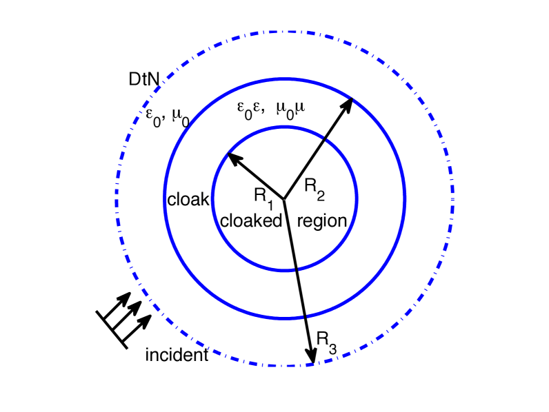
Figure 1. Schematic illustration of the circular cloak

Consider the free space time-harmonic Maxwell equations with angular frequency $\omega$ in the original $(\rho,\theta,z)$-coordinates:

$$\nabla\times{\boldsymbol{E}}-{\rm i}\omega\mu_{0}{\boldsymbol{H}}=0,\quad\nabla\times{\boldsymbol{H}}+{\rm i}\omega\varepsilon_{0}{\boldsymbol{E}}=0,\;\;\;{\rm in}\;\;{\mathbb{R}}^{3},$$ (2)

where a $e^{-{\rm i}\omega t}$ (note: ${\rm i}$ is the complex unit) time dependence is assumed, and the permeability $\mu_{0}$ and permittivity $\varepsilon_{0}$ are positive constants. It is known that the Maxwell equations are form invariant under coordinate transformations. Following the approach in [47], we apply the mapping (1), together with an identity transformation for $\rho>R_{2},$ to (2), leading to the Maxwell equation in the new $(r,\theta,z)$-coordinates:

$$\nabla^{\prime}\times{\boldsymbol{E}}-{\rm i}\omega\mu_{0}{\boldsymbol{\mu}}{\boldsymbol{H}}=0,\quad\nabla^{\prime}\times{\boldsymbol{H}}+{\rm i}\omega\varepsilon_{0}{\boldsymbol{\varepsilon}}{\boldsymbol{E}}=0,\quad r>R_{1},$$ (3)

with anisotropic, singular material parameters given by

$${\boldsymbol{\varepsilon}}={\boldsymbol{\mu}}={\rm diag}(\varepsilon_{r},\varepsilon_{\theta},\varepsilon_{z}),\quad{\rm if}\;\;\;R_{1}<r<R_{2},$$ (4)

$${\boldsymbol{\varepsilon}}=\boldsymbol{\mu}={\boldsymbol{I}_{3}},\qquad\qquad\qquad\;{\rm if}\;\;\;r>R_{2},$$ (5)

where $\boldsymbol{I}_{3}$ is the $3\times 3$ identity matrix, and

$$\varepsilon_{r}=\mu_{r}=\frac{r-R_{1}}{r},\quad\varepsilon_{\theta}=\mu_{\theta}=\frac{r}{r-R_{1}},\quad\varepsilon_{z}=\mu_{z}=\Big{(}\frac{R_{2}}{R_{2}-R_{1}}\Big{)}^{2}\,\frac{r-R_{1}}{r}.$$ (6)

We refer to [8, 9] for a general framework for transformation optics.

It is free to set any values for the permeability and permittivity in the cloaked region: $r<R_{1}.$ Without loss of generality (cf. [47]), we set ${\boldsymbol{\varepsilon}}=\boldsymbol{\mu}={\boldsymbol{I}_{3}}$ for $r<R_{1}.$

In what follows, we consider the transverse-electric (TE) polarised electromagnetic field, that is, the electrical field only exists in the $z$ direction: $\boldsymbol{E}=(0,0,u)^{t}.$ Then by the first equation of (3), we have

$$\boldsymbol{H}=(H_{1},H_{2},0)^{t}=\frac{1}{{\rm i}\omega\mu_{0}}\begin{cases}\Big{(}\dfrac{1}{r-R_{1}}\dfrac{\partial u}{\partial\theta},-\dfrac{r-R_{1}}{r}\dfrac{\partial u}{\partial r},0\Big{)}^{t},\quad&{\rm if}\;\;R_{1}<r<R_{2},\\[12.0pt] \Big{(}\dfrac{1}{r}\dfrac{\partial u}{\partial\theta},-\dfrac{\partial u}{\partial r},0\Big{)}^{t},\quad&{\rm if}\;\;r<R_{1}\;\;{\rm or}\;\;r>R_{2}.\end{cases}$$ (7)

Eliminating $\boldsymbol{H}$ from the Maxwell equations (3), we obtain the two-dimensional Helmholtz equations in polar coordinates:

$${\mathcal{L}}_{0}[u]:=\frac{1}{r}\frac{\partial}{\partial r}\Big{(}r\frac{\partial u}{\partial r}\Big{)}+\frac{1}{r^{2}}\frac{\partial^{2}u}{\partial\theta^{2}}+k^{2}u=0,\qquad\;{\rm if}\;\;r<R_{1}\;\;{\rm or}\;\;r>R_{2};$$ (8)

$${\mathcal{L}}_{1}[u]:=\frac{1}{r-R_{1}}\frac{\partial}{\partial r}\Big{(}(r-R_{1})\frac{\partial u}{\partial r}\Big{)}+\frac{1}{(r-R_{1})^{2}}\frac{\partial^{2}u}{\partial\theta^{2}}+k^{2}b^{2}u=0,\quad{\rm if}\;\;R_{1}<r<R_{2},$$ (9)

for all $\theta\in[0,2\pi),$ where

$$k=\omega\sqrt{\varepsilon_{0}\mu_{0}},\quad b={R_{2}}/{(R_{2}-R_{1})}.$$ (10)

Conventionally, we impose the Sommerfeld radiation boundary condition for the scattering wave: $u_{\rm sc}=u-u_{\rm in}$ (where $u_{\rm in}$ is the incident wave, i.e., $\boldsymbol{E}_{\rm in}=(0,0,u_{\rm in})^{t}$, see Figure 1):

$$\partial_{r}u_{\rm sc}-{\rm i}k\,u_{\rm sc}=O(r^{-1/2}).$$ (11)

2.2. Exact DtN boundary condition, transmission conditions and CBCs

We now consider the boundary and transmission conditions to achieve perfect concealment of waves.

Starting with the outmost, we adopt the domain truncation by imposing an artificial boundary condition at $r=R_{3}>R_{2}$ using the exact Dirichlet-to-Neumann (DtN) technique (see, e.g., [22, 45]):

$$\partial_{r}u_{\rm sc}-{\mathcal{T}}_{R_{3}}u_{\rm sc}=0\quad{\rm at}\;\;r=R_{3},$$ (12)

where the DtN map ${\mathcal{T}}_{R_{3}}$ is defined as

$${\mathcal{T}}_{R_{3}}\psi=\sum_{|m|=0}^{\infty}\frac{k{H_{m}^{(1)}}^{\prime}(kR_{3})}{H_{m}^{(1)}(k_{0}R_{3})}\hat{\psi}_{m}e^{{\rm i}m\theta},\quad\hat{\psi}_{m}=\frac{1}{2\pi}\int_{0}^{2\pi}\psi(R_{3},\theta)e^{-{\rm i}m\theta}d\theta,$$ (13)

and $H_{m}^{(1)}$ is the Hankel function of the first kind. This yields the exact artificial boundary conditions of the total field:

$$\partial_{r}u-{\mathcal{T}}_{R_{3}}u=\partial_{r}u_{\rm in}-{\mathcal{T}}_{R_{3}}u_{\rm in}:=g\quad{\rm at}\;\;r=R_{3}.$$ (14)

Remark $2.1$. The exact DtN boundary condition is global in the physical space (due to the involvement of a Fourier series), but it is local in the expansion coefficient space. Given the geometry of the cloak, we can fully take this advantage in both simulation and analysis. ∎

For clarity of exposition, let us denote

$$R_{0}=0;\;\;\;I_{i}=(R_{i},R_{i+1}),\quad\Omega_{i}=I_{i}\times[0,2\pi),\quad i=0,1,2;\quad\Omega=\bigcup_{i=0}^{2}\Omega_{i}.$$ (15)

Correspondingly, we define

$$\boldsymbol{H}^{i}=\boldsymbol{H}|_{\Omega_{i}},\quad\boldsymbol{E}^{i}=\boldsymbol{E}|_{\Omega_{i}},\quad u^{i}=u|_{I_{i}},\quad i=0,1,2.$$ (16)

The conditions at the material interface $r=R_{2}$ are the standard transmission conditions, that is, the tangential components of $\boldsymbol{E}$ and $\boldsymbol{H}$ are continuous across the interface (see, e.g., [46, Sec. 1.5] and [43]):

$$\boldsymbol{n}\times(\boldsymbol{E}^{1}-\boldsymbol{E}^{2})=\boldsymbol{0},\quad\boldsymbol{n}\times(\boldsymbol{H}^{1}-\boldsymbol{H}^{2})=\boldsymbol{0}\quad{\rm at}\;\;r=R_{2},$$ (17)

where $\boldsymbol{n}$ is the outer unit normal. A direct calculation

from (7), leads to

$$u^{1}-u^{2}=0,\quad b^{-1}\partial_{r}u^{1}-\partial_{r}u^{2}=0\quad{\rm at}\;\;r=R_{2}.$$ (18)

As mentioned in the introductory section, how to impose suitable conditions so that there is no wave propagating into the cloaked region, appears unsettled. The analysis in Ruan et al. [48] implies that

$$\boldsymbol{E}^{1}\not=\boldsymbol{0},\quad\boldsymbol{n}\times(\boldsymbol{E}^{0}-\boldsymbol{E}^{1})\not=\boldsymbol{0}\quad{\rm at}\;\;r=R_{1},$$ (19)

while the tangential component is continuous across the inner boundary, namely,

$$\boldsymbol{n}\times(\boldsymbol{H}^{0}-\boldsymbol{H}^{1})=\boldsymbol{0}\quad{\rm at}\;\;r=R_{1}.$$ (20)

Zhang et al. [62] demonstrates that the exotic physical effect (19) is attributed to the surface current induced by the singular transformation.

We find from (7) and (20) that

$$\lim_{r\to R_{1}}\Big{(}\partial_{r}u^{0}-\frac{r-R_{1}}{r}\partial_{r}u^{1}\Big{)}=0,\quad$$ (21)

which implies

$$\partial_{r}u^{0}(R_{1})=0,\quad\partial_{r}u^{1}(R_{1})\;\;\text{is finite}.$$ (22)

Remark $2.2$. To shield the wave from propagating into the cloaked region, the PMC condition (i.e., $\boldsymbol{n}\times\boldsymbol{H}^{1}=\boldsymbol{0}$), is imposed in many simulations in Cartesian coordinates (see, e.g., [13, 62, 32]). Unfortunately, we infer from (22) that in the polar coordinates, the PMC condition (equivalent to $\partial_{r}u^{1}(R_{1})$ being finite) does not lead to an independent condition. ∎

At this point, one condition is lacking at the inner boundary. Our viewpoint is that the electromagnetic fields in the original coordinates must still be finite after the coordinate transformation. Therefore, letting $r\to R_{1}^{+}$ in (7) yields

$$\frac{\partial u^{(1)}}{\partial\theta}(R_{1},\theta)=0,\quad\theta\in[0,2\pi).$$ (23)

We reiterate that this condition can be viewed as the essential “pole condition”, arisen from the polar transformation (singular at the origin). Note that the “pole” condition is imposed so that the solution in the polar coordinates has desired regularity, when it is transformed back to Cartesian coordinates (see, e.g., [19, 6]). As shown in [50, 51], the condition: $\partial_{\theta}u(0,\theta)=0$ is essential for spectral-accurate computations. Indeed, such a notion can be extended to other singular transformations (see e.g., [54]). In this context, the transformation (1) spans the origin to the circle $r=R_{1},$ so the essential “pole” condition is transplanted to $r=R_{1}^{+}.$

The problem of interest is summarised as follows:

$${\mathcal{L}}_{0}[u^{0}]=0\;\;\;{\rm in}\;\;\Omega_{0};\quad\partial_{\theta}u^{0}(0,\theta)=\partial_{r}u^{0}(R_{1},\theta)=0;$$ (24)

$${\mathcal{L}}_{1}[u^{1}]=0\;\;\;{\rm in}\;\;\Omega_{1};\quad\partial_{\theta}u^{1}(R_{1},\theta)=0;$$ (25)

$$u^{1}=u^{2},\quad b^{-1}\partial_{r}u^{1}=\partial_{r}u^{2}\quad{\rm at}\;\;r=R_{2},$$ (26)

$${\mathcal{L}}_{0}[u^{2}]=0\;\;\;{\rm in}\;\;\Omega_{2};\quad\partial_{r}u^{2}-{\mathcal{T}}_{R_{3}}u^{2}=g\quad{\rm at}\;\;r=R_{3};$$ (27)

for all $\theta\in[0,2\pi).$ Note that (i) the operators ${\mathcal{L}}_{0}$ and ${\mathcal{L}}_{1}$ are defined in (8)-(9); (ii) the EPC: $\partial_{\theta}u^{0}(0,\theta)=0$ is imposed at the origin due to the singular polar transformation; and (iii) the source of the system is the incident wave in the data $g$ (cf. (14)).

Remarkably, under the condition (21), the subproblem (24) is decoupled from (25)-(27). Moreover, we can show that $u^{0}\equiv 0$ is the unique solution, if the wave number $k$ is not an eigenvalue of the Bessel operator with the boundary conditions in (28). Indeed, we write $u^{0}(r,\theta)=\sum_{|m|=0}^{\infty}\hat{u}_{m}^{0}(r)e^{{\rm i}m\theta}.$ Then (24) reduces to

$$\begin{split}&\frac{1}{r}\frac{d}{dr}\Big{(}r\frac{d\hat{u}_{m}^{0}}{dr}\Big{)}-\frac{m^{2}}{r^{2}}\hat{u}_{m}^{0}+k^{2}\hat{u}_{m}^{0}=0,\quad 0<r<R_{1};\\ &\hat{u}_{m}^{0}(0)=0,\;\;{\rm if}\;\;m\not=0;\quad\frac{d}{dr}\hat{u}_{m}^{0}(R_{1})=0,\;\;\;m=0,\pm 1,\cdots.\end{split}$$ (28)

We claim from the Sturm-Liouville theory of the Bessel operator (see, e.g., [11, 3]) the following conclusion. Proposition $2.1$. If $k$ is not an eigenvalue of the Bessel problem (28), or equivalently, $J_{m}^{\prime}(kR_{1})\not=0$ for any model $m,$ then we have $\hat{u}_{m}^{0}\equiv 0$ for every $m,$ so the solution of (24) $u^{0}\equiv 0.$ ∎

We see that with a reasonable assumption on the frequency of the incident wave, the cloak can perfectly shield the waves from penetrating into the cloaked region.

2.3. Fourier-Legendre-spectral-element method

We next present an accurate and efficient numerical method for solving (25)-(27). Observe from (14) that the DtN boundary condition in (27) is global in the physical space, but it is local in the frequency space of Fourier expansion. It is therefore advantageous to use Fourier spectral approximation in $\theta$-direction, and Legendre spectral-element method in $r$-direction.

We expand the solution and given data in Fourier series:

$$\big{\{}u^{j}(r,\theta),g(\theta)\}=\sum_{|m|=0}^{\infty}\big{\{}\hat{u}_{m}^{j}(r),\hat{g}_{m}\big{\}}e^{{\rm i}m\theta},\quad j=1,2.$$ (29)

Then (25)-(27) reduce to a sequence of one-dimensional equations:

$$\frac{1}{r-R_{1}}\frac{d}{dr}\Big{(}(r-R_{1})\frac{d\hat{u}_{m}^{1}}{dr}\Big{)}-\frac{m^{2}}{(r-R_{1})^{2}}\hat{u}_{m}^{1}+k^{2}b^{2}\hat{u}_{m}^{1}=0,\quad R_{1}<r<R_{2};$$ (30)

$$\hat{u}_{m}^{1}(R_{1})=0,\;\;{\rm if}\;\;m\neq 0;\quad\hat{u}_{m}^{1}(R_{2})=\hat{u}_{m}^{2}(R_{2}),\quad b^{-1}\frac{d}{dr}\hat{u}_{m}^{1}(R_{2})=\frac{d}{dr}\hat{u}_{m}^{2}(R_{2});$$ (31)

$$\frac{1}{r}\frac{d}{dr}\Big{(}r\frac{d\hat{u}_{m}^{2}}{dr}\Big{)}-\frac{m^{2}}{r^{2}}\hat{u}_{m}^{2}+k^{2}\hat{u}_{m}^{2}=0,\quad R_{2}<r<R_{3};$$ (32)

$$\Big{(}\frac{d}{dr}-{\mathcal{T}}_{m,k}\Big{)}\hat{u}_{m}^{2}(R_{3})=\hat{g}_{m},\quad\text{where}\;\;{\mathcal{T}}_{m,k}:=\frac{k{H_{m}^{(1)}}^{\prime}(kR_{3})}{H_{m}^{(1)}(kR_{3})}.$$ (33)

Note that the global DtN boundary condition is decoupled for each mode $m,$ and by the property of the Hankel function, we have ${\mathcal{T}}_{-m,k}={\mathcal{T}}_{m,k}$ (see [53, (2.32)]).

Hereafter, let $\Lambda=(a,b)$ and $\varpi(x)>0$ be a generic weight function on $\Lambda,$ which is absolutely integrable. Let $H^{s}_{\varpi}(\Lambda)$ be the weighted Sobolev space as defined in Admas [2]. In particular, $L^{2}_{\varpi}(\Lambda)=H^{0}_{\varpi}(\Lambda)$ with the inner product $(\cdot,\cdot)_{\varpi}$ and norm $\|\cdot\|_{\varpi}.$ We drop the weight function, whenever $\varpi=1.$

Let $I_{1}=(R_{1},R_{2})$ and $I_{2}=(R_{2},R_{3})$ as before, and let $I=(R_{1},R_{3}).$ Define the weight function $\omega$ and the piecewise constant function $\rho$:

$$\omega(r)=\begin{cases}r-R_{1},\quad&{\rm if}\;\;r\in I_{1},\\ r,\quad&{\rm if}\;\;r\in I_{2},\end{cases}\quad\rho=\begin{cases}b^{2},\quad&{\rm if}\;\;r\in I_{1},\\ 1,\quad&{\rm if}\;\;r\in I_{2}.\end{cases}$$ (34)

Recall that $b=R_{2}/(R_{2}-R_{1})$ as defined in (10). The weak form of (30)-(33) is to find $\hat{u}_{m}\in Y_{m}(I)$ for each mode $m,$ such that

$$\begin{split}{\mathcal{B}}_{m}(\hat{u}_{m},v):=&(\hat{u}_{m}^{\prime},v^{\prime})_{\omega}+m^{2}(\hat{u}_{m},v)_{\omega^{-1}}-k^{2}(\rho\hat{u}_{m},v)_{\omega}\\ &-R_{3}{\mathcal{T}}_{m,k}\,\hat{u}_{m}(R_{3})\bar{v}(R_{3})=R_{3}\hat{g}_{m}\bar{v}(R_{3}),\quad\forall v\in Y_{m}(I),\end{split}$$ (35)

where $\bar{v}$ is the complex conjugate of $v.$ We show in Appendix A the following proposition on the well-posedness of (35). Proposition $2.2$. For each mode $m,$ the problem (35) has a unique solution $\hat{u}_{m}\in Y_{m}(I).$

We now discuss the numerical solution of (35). Let ${\mathbb{P}}_{N}$ be the complex-valued polynomials of degree at most $N,$ and let $\boldsymbol{N}=(N_{1},N_{2}).$ We introduce the approximation space:

$$Y_{m}^{\boldsymbol{N}}(I)=\big{\{}u\in Y_{m}(I)\,:\,u|_{I_{i}}\in{\mathbb{P}}_{N_{i}},\;\;i=1,2\big{\}},$$ (36)

where the functions are continuous across $r=R_{2}$ (cf. (31)). Given a cut-off number $M>0,$ the FLSEM approximation to the solution of (25)-(27) is

$$u_{M}^{\boldsymbol{N}}(r,\theta)=\sum_{|m|=0}^{M}\hat{u}_{m}^{\boldsymbol{N}}(r)e^{{\rm i}m\theta},\;\;\;$$ (37)

where $\{\hat{u}_{m}^{\boldsymbol{N}}\}$ are computed from the Legendre-spectral-element approximation to (35), that is, find $\hat{u}_{m}^{\boldsymbol{N}}\in Y_{m}^{\boldsymbol{N}}(I)$ such that

$$\begin{split}{\mathcal{B}}_{m}(\hat{u}_{m}^{\boldsymbol{N}},v)=R_{3}\hat{g}_{m}\bar{v}(R_{3}),\quad\forall v\in Y_{m}^{\boldsymbol{N}}(I),\quad 0\leq|m|\leq M.\end{split}$$ (38)

Remark $2.3$. We can apply the same argument as for Proposition $2.2$ to show that (38) admits a unique solution in $Y_{m}^{\boldsymbol{N}}(I)$. ∎

For each mode $m,$ the two-domain spectral-element scheme (38) can be implemented efficiently by using the modal Legendre polynomial basis and the Schur complement technique (cf. [24]). Here, we omit the details. We provide in section 4 ample numerical results to demonstrate that our proposed CBCs and FLSEM, leads to accurate simulations of the ideal circular cylindrical cloak.

3. Elliptic cylindrical cloaks

The elliptic cylindrical cloaks have been much less studied (see, e.g., [25, 27, 10]), compared with intensive investigations of the circular cylindrical cloaks. Though it is straightforward to extend the coordinate transformation in [47] to the elliptic case, the coordinate transformation possesses quite different nature of singularity. Thus, much care is needed to impose CBCs, as to be shown shortly.

3.1. Elliptic coordinates and Mathieu functions

To formulate the problem and algorithm, we briefly review the elliptic coordinates and the related angular and radial Mathieu functions. The elliptic coordinates $(\xi,\eta)$ are related to the Cartesian coordinates ${\boldsymbol{x}}=(x,y)$ by

$$x=a\cosh\xi\cos\eta,\quad y=a\sinh\xi\sin\eta,\quad a>0,$$ (39)

where $\xi\in[0,\infty)$ and $\eta\in[0,2\pi).$ The coordinate lines are confocal ellipses (of constant $\xi$) and hyperbolae (of constant $\eta$) with foci fixed at $-a$ and $a$ on the $x$-axis. The scale factors and the Jacobian of the elliptic coordinate system are

$$h=h_{\xi}=h_{\eta}=a\sqrt{\cosh^{2}\xi-\cos^{2}\eta},\quad J=h_{\xi}h_{\eta}=h^{2}.$$ (40)

The (angular) Mathieu equation reads (cf. [1]):

$$\frac{d^{2}\Phi}{d\eta^{2}}+(\lambda-2q\cos 2\eta)\Phi=0\;\;{\rm with}\;\;q=\frac{a^{2}k^{2}}{4},$$ (41)

where $\lambda$ is the separation constant. The angular Mathieu equation (41) supplemented with periodic boundary conditions admits a countable set of eign-pairs :

$$\big{\{}\lambda_{m}^{\rm c}(q),\;{\rm ce}_{m}(\eta;q)\big{\}}_{m=0}^{\infty},\quad\big{\{}\lambda_{m}^{\rm s}(q),\;{\rm se}_{m}(\eta;q)\big{\}}_{m=1}^{\infty}.$$ (42)

Note that the symbols “${\rm ce}$” and “${\rm se}$”, abbreviation of “cosine-elliptic” and “sine-elliptic”, were first introduced in [59]. To facilitate the analysis afterwards, let us denote

$$\tilde{\lambda}_{m}^{\rm c}(q):=\lambda_{m}^{\rm c}(q)+2q,\quad\tilde{\lambda}_{m}^{\rm s}(q):=\lambda_{m}^{\rm s}(q)+2q.$$ (43)

Then for any fixed $q>0,$ from the standard Sturm-Liouville theory (cf. [11]), the eigenvalues are in order of

$$0<\tilde{\lambda}_{0}^{\rm c}(q)<\tilde{\lambda}_{1}^{\rm s}(q)<\tilde{\lambda}_{1}^{\rm c}(q)<\cdots<\tilde{\lambda}_{m}^{\rm s}(q)<\tilde{\lambda}_{m}^{\rm c}(q)<\cdots.$$ (44)

When $q=0,$ the Mathieu functions reduce to the trigonometric functions:

$${\rm ce}_{0}(\eta;0)=\frac{1}{\sqrt{2}};\quad{\rm ce}_{m}(\eta;0)=\cos(m\eta),\quad{\rm se}_{m}(\eta;0)=\sin(m\eta),\;\;\;m\geq 1,$$ (45)

and correspondingly, $\lambda_{m}^{\rm c}(0)=\lambda_{m}^{\rm s}(0)=m^{2}.$ Indeed, the angular Mathieu functions share many properties with their conterparts: cosines and sines. For example, ${\rm ce}_{m}(\eta;q)$ is an even function in $\eta,$ and ${\rm se}_{m}(\eta;q)$ is odd. They are $\pi$-periodic when $m$ is even, and $2\pi$-periodic when $m$ is odd. Moreover, the set of Mathieu functions $\{{\rm ce}_{m},{\rm se}_{m+1}\}_{m=0}^{\infty}$ forms a complete orthogonal system in $L^{2}(0,2\pi)$ (cf. [41, 1]):

$$\int_{0}^{2\pi}{\rm ce}_{m}\,{\rm ce}_{n}\,d\eta=\int_{0}^{2\pi}{\rm se}_{m}\,{\rm se}_{n}\,d\eta=\pi\delta_{mn};\quad\int_{0}^{2\pi}{\rm ce}_{m}\,{\rm se}_{n}\,d\eta=0.$$ (46)

The radial (or modified) Mathieu equation (cf. [1]):

$$\frac{d^{2}\Psi}{d\xi^{2}}-(\lambda-2q\cosh 2\xi)\Psi=0,$$ (47)

plays an analogous role as the Bessel equation in the polar coordinates. Like the Bessel functions, there are several types of radial Mathieu functions, but each type has even and odd versions, quite different notation is used to denote such functions in literature [41, 1]. In this paper, we adopt the notation and conventions in [1], where $\{{\rm Mc}_{m}^{(i)};{\rm Ms}_{m}^{(i)}\},i=1,2,3,4,$ correspond to the Bessel functions: $J_{m},Y_{m},H_{m}^{(1)},H_{m}^{(2)}$ in [56], respectively. In what follows, we shall just use the radial Mathieu functions of the first kind $\{{\rm Mc}_{m}^{(1)}(\xi;q);{\rm Ms}_{m}^{(1)}(\xi;q)\}$, and the Mathieu-Hankel functions: $\{{\rm Mc}_{m}^{(3)}(\xi;q);{\rm Ms}_{m}^{(3)}(\xi;q)\}.$ Both types satisfy (47) with $\lambda=\lambda_{m}^{\rm c}$ and $\lambda=\lambda_{m}^{\rm s}$ for ${\rm Mc}_{m}$ and ${\rm Ms}_{m},$ respectively.

3.2. Maxwell equations for ideal elliptic cylindrical cloak

Following the idea of Pendry et al. [47], a coordinate transformation, which compresses the elliptic region $0\leq\zeta<\xi_{2}$ into the elliptic annular region $0<\xi_{1}<\xi<\xi_{2},$ was extended to devise an elliptic cylindrical cloak (see e.g., [40, 10]):

$$\xi=\frac{\zeta}{d}+\xi_{1},\quad\eta=\eta,\quad z=z\;\;\;{\rm with}\;\;\;d=\frac{\xi_{2}}{\xi_{2}-\xi_{1}},$$ (48)

where $(\zeta,\eta,z)$ is the elliptic-cylindrical coordinates in the original space, and $(\xi,\eta,z)$ is the coordinates of the transformed space. This leads to the study of the time-harmonic Maxwell equations in the transformed space with new material parameters:

$$\nabla\times{\boldsymbol{E}}-{\rm i}\omega\mu_{0}{\boldsymbol{\mu}}{\boldsymbol{H}}=0,\quad\nabla\times{\boldsymbol{H}}+{\rm i}\omega\varepsilon_{0}{\boldsymbol{\varepsilon}}{\boldsymbol{E}}=0,\;\;\;\xi>\xi_{1},$$ (49)

where we have

$$\begin{split}&{\boldsymbol{\varepsilon}}={\boldsymbol{\mu}}={\rm diag}(\varepsilon_{\xi},\varepsilon_{\eta},\varepsilon_{z}),\;\;{\rm if}\;\;\xi_{1}<\xi<\xi_{2};\quad{\boldsymbol{\varepsilon}}={\boldsymbol{\mu}}=\boldsymbol{I}_{3},\;\;{\rm if}\;\;\xi>\xi_{2},\end{split}$$ (50)

with the components in the cloak (cf. [40]), given by

$$\varepsilon_{\xi}=\mu_{\xi}=\frac{1}{d},\quad\varepsilon_{\eta}=\mu_{\eta}=d,\quad\varepsilon_{z}=\mu_{z}=d\frac{\cosh^{2}(d(\xi-\xi_{1}))-\cos^{2}\eta}{\cosh^{2}\xi-\cos^{2}\eta}.$$ (51)

As with the circular case, we consider the transverse-electric (TE) polarised electromagnetic field with $\boldsymbol{E}=(0,0,v)^{t}.$ Like (7), the magnetic field in this context takes the form:

$$\boldsymbol{H}=(H_{1},H_{2},0)^{t}=\frac{1}{{\rm i}\omega\mu_{0}}\begin{cases}\Big{(}\dfrac{d}{h}\dfrac{\partial v}{\partial\eta},-\dfrac{1}{dh}\dfrac{\partial v}{\partial\xi},0\Big{)}^{t},\quad&{\rm if}\;\;\xi_{1}<\xi<\xi_{2},\\[12.0pt] \Big{(}\dfrac{1}{h}\dfrac{\partial v}{\partial\eta},-\dfrac{1}{h}\dfrac{\partial v}{\partial\xi},0\Big{)}^{t},\quad&{\rm if}\;\;\xi>\xi_{2}\;\;{\rm or}\;\;0<\xi<\xi_{1}.\end{cases}$$ (52)

With the above polarisation, we eliminate $\boldsymbol{H}$ and obtain the Helmholtz equations, together with exact DtN boundary at the outer ellipse $\xi=\xi_{3}(>\xi_{2}),$ in elliptic coordinates:

$$\big{(}{d^{-2}}\partial^{2}_{\xi}+\partial^{2}_{\eta}\big{)}v+k^{2}a^{2}\big{(}\cosh^{2}(d(\xi-\xi_{1}))-\cos^{2}\eta\big{)}v=0\quad\;{\rm in}\;\;\Lambda_{1};$$ (53a)

$$\big{(}\partial^{2}_{\xi}+\partial^{2}_{\eta}\big{)}v+k^{2}a^{2}\big{(}\cosh^{2}\xi-\cos^{2}\eta\big{)}v=0\qquad\qquad{\rm in}\;\;\Lambda_{0}\cup\Lambda_{2};$$ (53b)

$$(\partial_{\xi}-{\mathbb{T}}_{\xi_{3}})v=\phi\quad\;\;{\rm at}\;\;\xi=\xi_{3},$$ (53c)

where

$$k=\omega\sqrt{\varepsilon_{0}\mu_{0}};\quad\Lambda_{i}:=(\xi_{i},\xi_{i+1})\times[0,2\pi),\;\;\;i=0,1,2\;\;{\rm with}\;\;\xi_{0}:=0,$$

and ${\mathbb{T}}_{\xi_{3}}$ is the DtN map (cf. [22, 17]), given by

$$\begin{split}&{\mathbb{T}}_{\xi_{3}}v=\sum_{m=0}^{\infty}\frac{\partial_{\xi}{\rm Mc}_{m}^{(3)}(\xi_{3};q)}{{\rm Mc}_{m}^{(3)}(\xi_{3};q)}\hat{v}^{\rm c}_{m}(\xi_{3})\,{\rm ce}_{m}(\eta;q)+\sum_{m=1}^{\infty}\frac{\partial_{\xi}{\rm Ms}_{m}^{(3)}(\xi_{3};q)}{{\rm Ms}_{m}^{(3)}(\xi_{3};q)}\hat{v}^{\rm s}_{m}(\xi_{3})\,{\rm se}_{m}(\eta;q),\end{split}$$ (54)

with

$$\hat{v}_{m}^{\rm c}(\xi_{3})=\frac{1}{\pi}\int_{0}^{2\pi}v(\xi_{3},\eta)\,{\rm ce}_{m}(\eta;q)\,d\eta,\quad\hat{v}_{m}^{\rm s}(\xi_{3})=\frac{1}{\pi}\int_{0}^{2\pi}v(\xi_{3},\eta)\,{\rm se}_{m}(\eta;q)\,d\eta.$$ (55)

Note that in (53c), $\phi$ is induced by the incident wave, i.e., $\phi=(\partial_{\xi}-{\mathbb{T}}_{\xi_{3}})v_{\rm in}.$

Naturally, we impose continuity of the tangential components of $\boldsymbol{E}$ and $\boldsymbol{H}$ across the elliptic interface $\xi=\xi_{2},$ leading to the transmission conditions as with (18):

$$v^{1}=v^{2},\quad d^{-1}\partial_{\xi}v^{1}=\partial_{\xi}v^{2},\quad{\rm at}\;\;\xi=\xi_{2},$$ (56)

where for clarity, we denote $v^{i}=v|_{\Lambda_{i}}$ for $i=0,1,2.$

The critical issue is the imposition of CBCs at the inner boundary $\xi=\xi_{1}.$ To tackle this, we decompose the solution and data into ce- and se-components as follows:

$$\begin{split}\big{\{}v;\,\phi\}&=\sum_{m=0}^{\infty}\big{\{}\hat{v}^{\rm c}_{m}(\xi);\,\hat{\phi}^{\rm c}_{m}\big{\}}{\rm ce}_{m}(\eta;q)+\sum_{m=1}^{\infty}\big{\{}\hat{v}^{\rm s}_{m}(\xi);\,\hat{\phi}^{\rm s}_{m}\big{\}}{\rm se}_{m}(\eta;q)\\ &:=\big{\{}v_{\rm ce};\,\phi_{\rm ce}\}+\big{\{}v_{\rm se};\,\phi_{\rm se}\}.\end{split}$$ (57)

Correspondingly, the polarized $\boldsymbol{E}$ and $\boldsymbol{H}$ fields are split into two components: $\boldsymbol{E}=\boldsymbol{E}_{{\rm ce}}+\boldsymbol{E}_{{\rm se}}$ and $\boldsymbol{H}=\boldsymbol{H}_{\rm ce}+\boldsymbol{H}_{\rm se}.$ Following the analytic study in [10] and the $\delta$-perturbation analysis in [48], it is necessary to require the tangential component of $\boldsymbol{H}_{{\rm ce}}$ and $\boldsymbol{E}_{{\rm se}}$ continuous across the inner boundary $\xi=\xi_{1}$, leading to

$$v^{0}_{\rm se}=v^{1}_{\rm se},\quad d^{-1}\partial_{\xi}v^{0}_{\rm ce}=\partial_{\xi}v^{1}_{\rm ce}\quad{\rm at}\;\;\xi=\xi_{1}.$$ (58)

Nevertheless, we are short of one condition for each component. Like the derivation of (23) in the circular case, we require the fields in the original space to be still finite in the transformed space, leading to the essential “pole” conditions. since the singularity of the transformation (48) only occurs at two points $(\xi_{1},0)$ and $(\xi_{1},\pi),$ as opposite to the circular case, taking limit $\xi\to\xi_{1}^{+}$ in (52), leads to

$$\partial_{\xi}v^{1}(\xi_{1},0)=\partial_{\xi}v^{1}(\xi_{1},\pi)=0,\quad\partial_{\eta}v^{1}(\xi_{1},0)=\partial_{\eta}v^{1}(\xi_{1},\pi)=0.$$ (59)

Using the property (cf. [1]):

$${\rm ce}_{m}^{\prime}(0;q)={\rm ce}_{m}^{\prime}(\pi;q)=0,\quad{\rm se}_{m}(0;q)={\rm se}_{m}(\pi;q)=0,$$ (60)

we find from (57) that (59) is equivalent to

$$\partial_{\xi}v^{1}_{\rm ce}(\xi_{1},0)=0,\quad v^{1}_{\rm se}(\xi_{1},0)=0.$$ (61)

We summarize the problem that models the ideal elliptic cylindrical cloak: given $\phi=\phi_{\rm ce}+\phi_{\rm se},$ find

$$v=v_{\rm ce}+v_{\rm se}\;\;{\rm with}\;\;v^{i}=v_{\rm ce}^{i}+v_{\rm se}^{i}=(v_{\rm ce}+v_{\rm se})|_{\Lambda_{i}},\;\;\;i=0,1,2,$$ (62)

satisfying the following systems.

• For the ${\rm ce}$-component in the cloaked region $\Lambda_{0}$:

  $$\big{(}\partial^{2}_{\xi}+\partial^{2}_{\eta}\big{)}v_{\rm ce}^{0}+k^{2}a^{2}\big{(}\cosh^{2}\xi-\cos^{2}\eta\big{)}v_{\rm ce}^{0}=0,\quad 0<\xi<\xi_{1};$$ (63)

  $$\partial_{\xi}v^{0}_{\rm ce}(0,0)=\partial_{\xi}v^{0}_{\rm ce}(\xi_{1},0)=0.$$ (64)

  Note that the essential pole condition at the origin is necessary, while $\partial_{\xi}v^{0}_{\rm ce}(\xi_{1},0)=0$ is derived from the second condition in (58) and (61).

• For the ${\rm ce}$-component in $\Lambda_{1}\cup\Lambda_{2}$:

  $$\big{(}d^{-2}\partial^{2}_{\xi}+\partial^{2}_{\eta}\big{)}v_{\rm ce}^{1}+k^{2}a^{2}\big{(}\cosh^{2}(d(\xi-\xi_{1}))-\cos^{2}\eta\big{)}v_{\rm ce}^{1}=0\quad\;{\rm in}\;\;\Lambda_{1};$$ (65a)

  $$\partial_{\xi}v^{1}_{\rm ce}(\xi_{1},0)=0;\quad\;\;v^{1}_{\rm ce}=v^{2}_{\rm ce},\quad d^{-1}\partial_{\xi}v^{1}_{\rm ce}=\partial_{\xi}v^{2}_{\rm ce}\qquad{\rm at}\;\;\;\xi=\xi_{2};$$ (65b)

  $$\big{(}\partial^{2}_{\xi}+\partial^{2}_{\eta}\big{)}v_{\rm ce}^{2}+k^{2}a^{2}\big{(}\cosh^{2}\xi-\cos^{2}\eta\big{)}v_{\rm ce}^{2}=0\qquad\qquad\;\;\;\;{\rm in}\;\;\Lambda_{2},$$ (65c)

  $$(\partial_{\xi}-{\mathbb{T}}_{\xi_{3}})v_{\rm ce}^{2}=\phi_{\rm ce}\qquad\;\;{\rm at}\;\;\xi=\xi_{3}.$$ (65d)

• The ${\rm se}$-component $v_{\rm se}$ satisfies the same equations in (i)-(ii) with $v_{\rm se}^{i}$ and $\phi_{\rm se}$ in place of $v_{\rm ce}^{i}$ and $\phi_{\rm ce},$ respectively, while (64) and the first condition in (65b) are respectively replaced by

  $$v^{0}_{\rm se}(0,0)=v^{0}_{\rm se}(\xi_{1},0)=0;\quad v^{1}_{\rm se}(\xi_{1},0)=0.$$ (66)

We see that $v_{\rm ce}^{0}$ and $v_{\rm se}^{0}$ are decoupled from $v_{\rm ce}^{i}$ and $v_{\rm se}^{i},\;i=1,2$. Indeed, using (41) and the expansion (57), the problem (63)-(64) reduces to

$$(\hat{v}_{m}^{\rm c})^{\prime\prime}(\xi)-\big{(}\lambda_{m}^{\rm c}-2q\cosh(2\xi)\big{)}\,\hat{v}_{m}^{\rm c}(\xi)=0,\quad 0<\xi<\xi_{1},$$ (67)

$$(\hat{v}_{m}^{\rm c})^{\prime}(0)=(\hat{v}_{m}^{\rm c})^{\prime}(\xi_{1})=0,$$ (68)

and similarly, we have

$$(\hat{v}_{m}^{\rm s})^{\prime\prime}(\xi)-\big{(}\lambda_{m}^{\rm s}-2q\cosh(2\xi)\big{)}\,\hat{v}_{m}^{\rm s}(\xi)=0,\quad 0<\xi<\xi_{1},$$ (69)

$$\hat{v}_{m}^{\rm s}(0)=\hat{v}_{m}^{\rm s}(\xi_{1})=0.$$ (70)

Similar to Proposition $2.1$, one deduces from the standard theory of ordinary differential equations (cf. [11, 3]) and also from the properties of Mathieu functions (cf. [1]) the following conclusions. Proposition $3.1.$ If $k$ and $\xi_{1}$ are chosen such that ${{\rm Mc}_{m}^{(1)}}^{\prime}(k\xi_{1})\not=0$ and ${{\rm Ms}_{m}^{(1)}}(k\xi_{1})\not=0$ for any mode $m,$ then we have $\hat{v}_{m}^{\rm c}=\hat{v}_{m}^{\rm s}\equiv 0$ for every $m,$ so the problem (63)-(64) and the problem of ${{\rm se}}$-component in $\Lambda_{0}$ with (66), both have only trivial solutions in the cloaked region. ∎

3.3. Mathieu-Legendre-spectral-element method

In what follows, we present an accurate and efficient numerical algorithm to simulate the ideal elliptic cylindrical cloak.

Using the Mathieu expansion in $\eta$-direction (see (57)), we obtain the system of the ${\rm ce}$-component in $\Lambda_{1}\cup\Lambda_{2}$:

$$-{d^{-2}}(\hat{v}_{m}^{\rm c})^{\prime\prime}(\xi)+\big{(}\tilde{\lambda}_{m}^{\rm c}-4q\cosh^{2}(d(\xi-\xi_{1}))\big{)}\hat{v}_{m}^{\rm c}=0,\quad\xi_{1}<\xi<\xi_{2};$$ (71a)

$$(\hat{v}_{m}^{\rm c})^{\prime}(\xi_{1})=0;\quad\hat{v}_{m}^{\rm c}(\xi_{2}^{-})=\hat{v}_{m}^{\rm c}(\xi_{2}^{+}),\;\;d^{-1}(\hat{v}_{m}^{\rm c})^{\prime}(\xi_{2}^{-})=(\hat{v}_{m}^{\rm c})^{\prime}(\xi_{2}^{+});$$ (71b)

$$-(\hat{v}_{m}^{\rm c})^{\prime\prime}(\xi)+\big{(}\tilde{\lambda}_{m}^{\rm c}-4q\cosh^{2}(\xi)\big{)}\hat{v}_{m}^{\rm c}(\xi)=0,\quad\xi_{2}<\xi<\xi_{3};$$ (71c)

$$\Big{(}\frac{d}{d\xi}-{\mathcal{D}}_{m}^{\rm c}\Big{)}\hat{v}_{m}^{\rm c}(\xi_{3})=\hat{\phi}_{m}^{\rm c},\quad\text{where}\;\;{\mathcal{D}}_{m}^{\rm c}:=\frac{{{\rm Mc}_{m}^{(3)}}^{\prime}(\xi_{3};q)}{{\rm Mc}_{m}^{(3)}(\xi_{3};q)}.$$ (71d)

Recall that $\tilde{\lambda}_{m}^{\rm c}:=\lambda_{m}^{\rm c}+2q>0$ (see (43)). The ${\rm se}$-component satisfies the same system with $\hat{v}_{m}^{\rm s}$, $\hat{\phi}_{m}^{\rm s}$ and $\tilde{\lambda}_{m}^{\rm s}$ in place of $\hat{v}_{m}^{\rm c}$, $\hat{\phi}_{m}^{\rm c}$ and $\tilde{\lambda}_{m}^{\rm c}$ in (71), respectively, while the first condition in (71b) and ${\mathcal{D}}_{m}^{\rm c}$ in (71d), are respectively replaced by

$$\hat{v}_{m}^{\rm s}(\xi_{1})=0,\quad{\mathcal{D}}_{m}^{\rm s}:=\frac{{{\rm Ms}_{m}^{(3)}}^{\prime}(\xi_{3};q)}{{\rm Ms}_{m}^{(3)}(\xi_{3};q)},\quad m\geq 1.$$ (72)

With a little abuse of notation, we still denote $I_{1}=(\xi_{1},\xi_{2}),$ $I_{2}=(\xi_{2},\xi_{3}),$ and $I=(\xi_{1},\xi_{3})$. To formulate the problem into a compact form (see (74) below), we introduce the piecewise functions:

$$\varpi=\begin{cases}d^{-1},\quad&{\rm if}\;\;\xi\in I_{1},\\ 1,\quad&{\rm if}\;\;\xi\in I_{2},\end{cases}\quad\chi=\begin{cases}\cosh^{2}(d(\xi-\xi_{1})),\quad&{\rm if}\;\;\xi\in I_{1},\\ \cosh^{2}\xi,\quad&{\rm if}\;\;\xi\in I_{2}.\end{cases}$$ (73)

Recall that $d=\xi_{2}/(\xi_{2}-\xi_{1})$ defined in (48). Apparently, these two functions are uniformly bounded.

The weak form of (71) is to find $\hat{v}_{m}^{\rm c}\in H^{1}(I)$ for each mode $m,$ such that

$$\begin{split}{\mathcal{B}}_{m}^{\rm c}(\hat{v}_{m}^{\rm c},\psi):=&(\varpi(\hat{v}_{m}^{\rm c})^{\prime},\psi^{\prime})+\tilde{\lambda}_{m}^{\rm c}(\varpi^{-1}\hat{v}_{m}^{\rm c},\psi)-4q(\varpi^{-1}\chi\hat{v}_{m}^{\rm c},\psi)\\ &-{\mathcal{D}}_{m}^{\rm c}\hat{v}_{m}^{\rm c}(\xi_{3})\bar{\psi}(\xi_{3})=\hat{\phi}_{m}^{\rm c}\bar{\psi}(\xi_{3}),\quad\forall\psi\in H^{1}(I),\;\;m=0,1,\cdots.\end{split}$$ (74)

Similarly, the weak form of the ${\rm se}$-component is to find $\hat{v}_{m}^{\rm s}\in{}_{0}H^{1}(I):=\{v\in H^{1}(I)\;:\;v(\xi_{1})=0\}$ for each mode $m,$ such that

$${\mathcal{B}}_{m}^{\rm s}(\hat{v}_{m}^{\rm s},\psi)=\hat{\phi}_{m}^{\rm s}\bar{\psi}(\xi_{3}),\quad\forall\psi\in{}_{0}H^{1}(I),\;\;m=1,2,\cdots,$$ (75)

where the bilinear form ${\mathcal{B}}_{m}^{\rm s}(\cdot,\cdot)$ is defined by replacing $\tilde{\lambda}_{m}^{\rm c}$ and ${\mathcal{D}}_{m}^{\rm c}$ in ${\mathcal{B}}_{m}^{\rm c}(\cdot,\cdot)$ by $\tilde{\lambda}_{m}^{\rm s}$ and ${\mathcal{D}}_{m}^{\rm s},$ respectively.

Like Proposition $2.2$, we next show the unique solvability of (74) and (75). We postpone its proof in Appendix B.

Proposition $3.2$. For each mode $m,$ the problem (74) (resp. (75)) has a unique solution $\hat{v}_{m}^{\rm c}\in H^{1}(I)$ (resp. $\hat{v}_{m}^{\rm s}\in{}_{0}H^{1}(I)$). ∎

We now introduce the numerical schemes. Define the approximation spaces:

$$Z_{m}^{\rm c,\boldsymbol{N}}(I)=\big{\{}v\in H^{1}(I)\,:v|_{I_{i}}\in{\mathbb{P}}_{N_{i}},\;\;i=1,2\big{\}};\quad Z_{m}^{\rm s,\boldsymbol{N}}(I)=Z_{m}^{\rm c,\boldsymbol{N}}(I)\cap H_{0}^{1}(I),$$ (76)

where $\boldsymbol{N}=(N_{1},N_{2}).$ Given a cut-off number $M>0$, the MLSEM approximation to the solution of (53) in $\Lambda_{1}\cup\Lambda_{2}$ is

$$v_{M}^{\boldsymbol{N}}(\xi,\eta)=\sum_{m=0}^{M}\hat{v}_{m}^{\rm c,\boldsymbol{N}}(\xi){\rm ce}_{m}(\eta;q)+\sum_{m=1}^{M}\hat{v}_{m}^{\rm s,\boldsymbol{N}}(\xi){\rm se}_{m}(\eta;q),$$ (77)

and $\{\hat{v}_{m}^{\rm c,\boldsymbol{N}},\hat{v}_{m}^{\rm s,\boldsymbol{N}}\}$ are computed from the Legendre-spectral-element schemes:  find $\hat{v}_{m}^{\rm c,\boldsymbol{N}}\in Z_{m}^{\rm c,\boldsymbol{N}}(I)$ such that

$${\mathcal{B}}_{m}^{\rm c}(\hat{v}_{m}^{\rm c,{\boldsymbol{N}}},\psi)=\hat{\phi}_{m}^{\rm c}\bar{\psi}(\xi_{3}),\quad\forall\psi\in Z_{m}^{\rm c,\boldsymbol{N}}(I),\quad 0\leq m\leq M,$$ (78)

and find $\hat{v}_{m}^{\rm s,\boldsymbol{N}}\in Z_{m}^{\rm s,\boldsymbol{N}}(I)$ such that

$${\mathcal{B}}_{m}^{\rm s}(\hat{v}_{m}^{\rm s,{\boldsymbol{N}}},\psi)=\hat{\phi}_{m}^{\rm s}\bar{\psi}(\xi_{3}),\quad\forall\psi\in Z_{m}^{\rm s,\boldsymbol{N}}(I),\quad 1\leq m\leq M.$$ (79)

Remark $3.1$. The unique solvability of (78)-(79) can be shown as the continuous problems in Proposition $3.2$. ∎

As with the circular case, the two-domain spectral-element scheme for each mode can be implemented by using the modal Legendre polynomial basis and the Schur complement technique (cf. [24]), but it is noteworthy that the resulted linear systems are full and dense due to the involvement of the non-polynomial weight function $\chi$ in (73).

4. Numerical results

In this section, we provide ample numerical results to demonstrate that our proposed approach produces accurate simulation of the ideal circular and elliptic cylindrical cloaks.

4.1. Circular cylindrical cloaks

Assuming that the incident wave is a plane wave with an incident angle $\theta_{0}$:

$$u_{{\rm in}}(r,\theta)=e^{{\rm i}kr\cos(\theta-\theta_{0})}=\sum_{|m|=0}^{\infty}{\rm i}^{m}{J}_{m}(kr)e^{{\rm i}m(\theta-\theta_{0})},$$ (80)

we can derive from the full-wave analysis in Ruan et al. [48] that the ideal cloaking problem admits the exact solution:

$$u(r,\theta)=\begin{cases}u_{{\rm in}}(b(r-R_{1}),\theta),\quad&{\rm if}\;\;R_{1}<r<R_{2},\\ u_{{\rm in}}(r,\theta),\quad&{\rm if}\;\;r>R_{2},\end{cases}$$ (81)

which vanishes in the cloaked region: $r<R_{1}.$

We first examine the numerical error: $E_{\boldsymbol{N}}=\smash{\max_{|m|\leq M}}\|\hat{u}_{m}-\hat{u}_{m}^{\boldsymbol{N}}\|_{\boldsymbol{N},\infty},$ where $\|\cdot\|_{\boldsymbol{N},\infty}$ denotes the maximum pointwise errors at the Legendre-Gauss-Lobatto points (with a linear transformation) used in each subinterval. In the computation, we take $M=70$ (so that the truncation error in $\theta$ direction is negligible), and choose $\theta_{0}=0$ and $(R_{1},R_{2},R_{3})=(0.2,0.6,1.0).$ In Figure 2 (left), we plot $\log_{10}(E_{\boldsymbol{N}})$ against $\boldsymbol{N}=(N,N)$ for $k=30,50,70.$ Observe that the error decays exponentially, when $N>N_{0}(k).$ The expected transition value $N_{0}(k)$ can be estimated by using the notion of “number-of-points-per-wavelength” (cf. [19]). Indeed, for large $k,$ the Bessel function behaves like (cf. [1]):

$$J_{m}(z)\sim\sqrt{\frac{2}{\pi z}}\cos\Big{(}z-\frac{m\pi}{2}-\frac{\pi}{4}\Big{)}.$$

We infer from the approxibility of Legendre polynomial expansions to trigonometric functions (cf. [19]) that as soon as

$$N>\frac{ek}{4}\max\{R_{2},R_{3}-R_{2}\}-\frac{1}{2},$$

the error begins to decay. Approximately, we take $N_{0}(k)$ to be ceiling round-off of this low bound. For $k=30,50,70,$ we find that $N_{0}=12,20,29,$ respectively, which agrees with the numerical results in Figure 2 (left). In Figure 2 (right), we plot the zeroth mode in the expansion (80) (see the solid line) versus the numerical approximation of $\hat{u}_{0}^{\boldsymbol{N}}(r)$ with $k=70$ and ${\boldsymbol{N}}=(50,50)$ (with marker “⁺”). We see that this mode is not continuous across the inner boundary $r=R_{1},$ which is the major reason for the surface currents (cf. [62]) and the violation of PEC condition (cf. (19)).

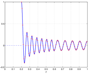
Figure 2. Left: errors against various $N$ for some samples of $k$. Right: the zeroth mode (in solid line) versus its numerical approximation $\hat{u}_{0}^{\boldsymbol{N}}$ (marked by “⁺”, with $k=70$ and ${\boldsymbol{N}}=(50,50)$).

We next illustrate the electric wave propagations and profiles under different incident angles and frequencies. In Figure 3, we depict the electric-field distributions (real and imaginary parts in the top row) simulated by the proposed FLSEM with $\theta_{0}=0,k=20,$ $(R_{1},R_{2},R_{3})=(0.2,0.6,1.0),$ $M=25$ and $\boldsymbol{N}=(20,20)$. We see that when a TE plane wave is incident on the circular cloak, it is completely guided and bent around the cloaked region without inducing any scattering waves. Moreover, the propagating wavefronts perfectly emerge from the other side of the cloaked region without any distortion, which are best testified to by profiles of ${\rm Re}\{u_{M}^{\boldsymbol{N}}\}$ and ${\rm Im}\{u_{M}^{\boldsymbol{N}}\}$ along $x$-axis (cf. (37)) in Figure 3. Once again, we observe that the real part is discontinuous across the inner boundary, attributed to the surface currents induced by the singular coordinate transformation (cf. [62]).

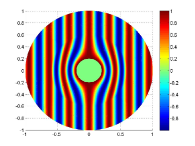
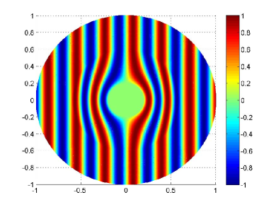
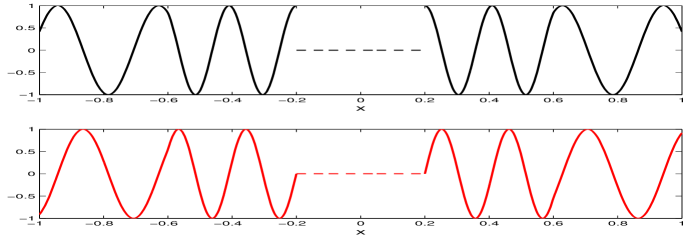
Figure 3. Row 1: real (left) and imaginary (right) parts of the electric-field distributions. Row 2-3: profiles of the real and imaginary parts of the electric-field along $x$-axis.

To further demonstrate the performance of the proposed approach, we set the incident angle $\theta_{0}=\pi/3,$ increase the incident frequency to $k=100$ and enlarge the cloaked region by taking $(R_{1},R_{2},R_{3})=(0.3,0.9,1.0).$ We depict in Figure 4 the same type of numerical results (obtained by the FLSEM with $M=120$ and $\boldsymbol{N}=(100,20)$) as in Figure 3. Again, the highly oscillatory oblique incident wave is perfectly steered by the cloaking layer, and completely shielded from the cloaked region. It is also worthwhile to point out that the exact boundary condition can be placed as close as possible to the cloak that can significantly reduce the number of grid points in the outermost artificial shell, especially when the incident frequency is high.

4.2. Wave generated by an external source

We now use an external source, compactly supported in the annulus $R_{2}<r<R_{3},$ as the wavemaker, and turn off the incident wave. More precisely, we modify (27) as

$${\mathcal{L}}_{0}[u^{2}]=f\;\;\;{\rm in}\;\;\Omega_{2};\quad(\partial_{r}-{\mathcal{T}}_{R_{3}})u^{2}=0\;\;\;{\rm at}\;\;r=R_{3}.$$ (82)

In this situation, there is no closed-form exact solution. In practice, we use the Guassian function in Cartesian coordinates:

$$f(x,y)=\alpha\;{\rm exp}\Big{(}{-\frac{(x-\beta)^{2}+(y-\kappa)^{2}}{2\gamma^{2}}}\Big{)},$$ (83)

where $\alpha,\beta,\kappa,\gamma$ are tuneable constants, and $\gamma$ is small. In the computation, we take $(R_{1},R_{2},R_{3})=(0.2,0.6,1.0)$, $\alpha=100$, $\beta=-0.8$, $\kappa=0$ and $\gamma=0.02.$ The source at $r=R_{3}$ is nearly zero. The plots of the electric-field distributions in Figure 5 are computed from the FLSEM with $k=40$, $M=40$ and $\boldsymbol{N}=(40,150).$ The non-plane waves generated by the source are smoothly bent and the cloak does not produce any scattering. We also observe from Figure 5 that the waves seamlessly pass through the outer artificial boundary without any reflecting.

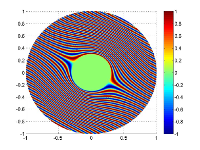
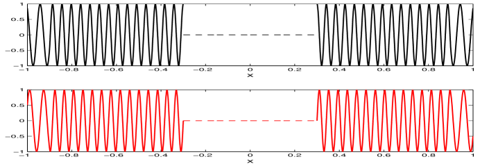
Figure 4. Row 1: real (left) and imaginary (right) parts of the electric-field distributions. Row 2-3: profiles of the real and imaginary parts of the electric-field along $\theta=\pi/3$.

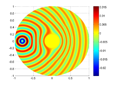
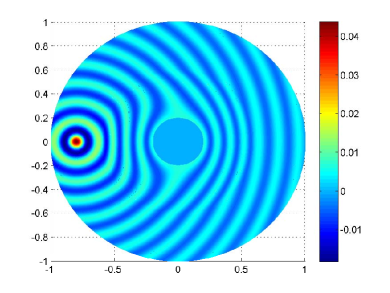
Figure 5. Electric-field distributions with an external source compactly supported in the outmost shell. Left: real part; right: imaginary part.

4.3. Elliptic cyindrical cloaks

We first consider an incident plane wave in (80), which, in the elliptic coordinates (cf. (39)), can be expanded in terms of Mathieu functions (cf. [42, P. 218]):

$$\begin{split}v_{\rm in}(\xi,\eta)&={\rm exp}({{\rm i}ka(\cosh\xi\cos\eta\cos\theta_{0}+\sinh\xi\sin\eta\sin\theta_{0})})\\ &=\sqrt{\frac{8}{\pi}}\sum_{m=0}^{\infty}{\rm i}^{m}{\rm Mc}_{m}^{(1)}(\xi;q){\rm ce}_{m}(\theta_{0};q){\rm ce}_{m}(\eta;q)\\ &\quad+\sqrt{\frac{8}{\pi}}\sum_{m=1}^{\infty}{\rm i}^{m}{\rm Ms}_{m}^{(1)}(\xi;q){\rm se}_{m}(\theta_{0};q){\rm se}_{m}(\eta;q).\end{split}$$ (84)

Note that when $q=0,$ it reduces to (80). Following [10], we obtain the exact solution for the ideal elliptic cloak similar to the circular case in (81):

$$v(\xi,\eta)=\begin{cases}v_{{\rm in}}(d(\xi-\xi_{1}),\eta),\quad&{\rm if}\;\;\xi_{1}<\xi<\xi_{2},\\ v_{{\rm in}}(\xi,\eta),\quad&{\rm if}\;\;\xi>\xi_{2},\end{cases}$$ (85)

which vanishes if $0<\xi<\xi_{1}.$

To illustrate the spectral accuracy of MLSEM, we tabulate in Table 1 the numerical errors $E_{\boldsymbol{N}}$ (defined as in the circular case) for different $\boldsymbol{N}=(N,N)$ and for several $k$. In the simulation, we take $a=0.6,\theta=0,(\xi_{1},\xi_{2},\xi_{3})=(0.7,1.3,1.5)$ and $M=70.$

Table 1. Convergence of MLSEM

	$k=30$	$k=50$	$k=70$
$N$	error	error	error
30	8.63E-07	2.75E-02	1.32
40	4.66E-12	8.42E-06	8.50E-02
50	9.03E-15	4.87E-10	3.52E-05
60	1.57E-14	2.27E-14	5.89E-09
70	1.66E-14	2.08E-14	2.73E-13

We next illustrate electric-field distributions. The circular cloak is perfectly symmetric, so the way of bending the waves is independent of the incident angle. However, as pointed out in, e.g., [40], the incident wave along the major axis (i.e., $\theta_{0}=0$) leads to significantly better cloaking effect with much less scattering and bears the greatest resemblance to the circular cloak, compared with other directions. Note that in [40], PEC condition was imposed at the inner boundary $\xi=\xi_{3}$ in the finite-element simulation, and the electric-field distributions exhibited observable scattering waves when the incident angle $\theta_{0}\not=0.$ However, using our proposed CBCs and numerical solver, the perfect cloaking effect can be achieved equally and no any scattering is induced for any incident angles. Apart from plotting the electric-field distributions, we also depict the time-averaged Poynting vector (cf. [46]):

$${\boldsymbol{S}}={\rm Re}\,\{{\boldsymbol{E}}\times{\boldsymbol{H}}^{*}\}/2,$$ (86)

which indicates the directional energy flux density. In Figures 6-8 (where $\theta_{0}=0,\pi/4,\pi$, respectively, and in all cases, $a=0.6$, $(\xi_{1},\xi_{2},\xi_{3})=(0.7,1.3,1.5),k=20$, $M=30$ and $\boldsymbol{N}=(20,20)$), we plot the real part of the electric-field distributions (note: the imaginary part behaves very similarly), and the corresponding Poynting vector fields. We find that the waves are again steered smoothly around the elliptic cloaked region without reflecting and scattering. We particularly look at the Poynting vectors in Figure 9, where the energy flux attempts to flow across $r=\xi_{1},$ but it is directed by the cloak. Once again, the surface current is induced on the cloaking interface as with the circular cloak. It is noteworthy that the incident wave perpendicular to the major axis (see Figure 9) is of particular interest, as the shape is like a slap and the waves are difficult to steer (cf. [25]). However, using our approach, the perfect concealment of waves can be achieved as with other incident angles.

Finally, we conduct a test by adding an external source (cf. Subsection 4.2), and turning off the incident wave. Accordingly, we modify (53b) and (53c) as

$$\big{(}\partial^{2}_{\xi}+\partial^{2}_{\eta}\big{)}v+k^{2}a^{2}\big{(}\cosh^{2}\xi-\cos^{2}\eta\big{)}v=f\;\;{\rm in}\;\;\Lambda_{2};\;\;(\partial_{\xi}-{\mathbb{T}}_{\xi_{3}})v=0\;\;{\rm at}\;\;\xi=\xi_{3},$$ (87)

where $f$ is compactly supported in the elliptic layer $\xi_{2}<\xi<\xi_{3}$. Like before, we take $f$ to be (83) with $\alpha=1000$, $\beta=0$, $\kappa=1.148$, $\gamma=0.01$. Figure 9 is computed from MLSEM with $k=20$, $M=30$ and $\boldsymbol{N}=(50,100)$ and illustrates the real (left) and imaginary (right) part of the electric-field distributions induced by external source. Once again, we see that the waves are smoothly bent without penetrating into the elliptic cloaked region. Moreover, the cloak does not induce any scattering, and indeed, we see the fields near the source totally unaffected.

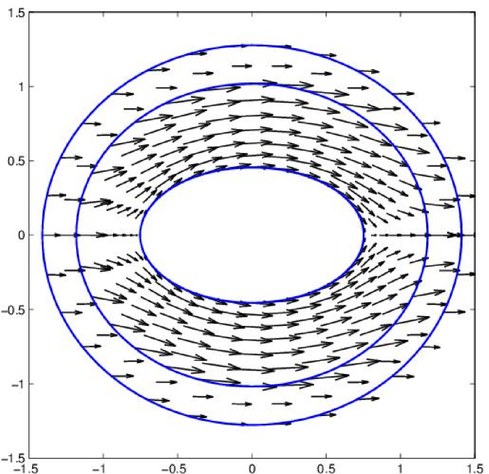
Figure 6. Real part of the electric-field distribution (left) and the related Poynting vector (right), where the incident angle $\theta_{0}=0$.

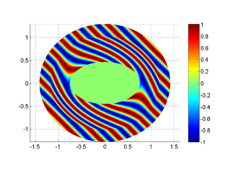
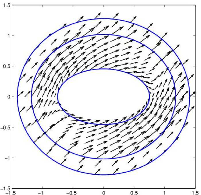
Figure 7. Real part of the electric-field distribution (left) and the related Poynting vector (right), where the incident angle $\theta_{0}={\pi}/{4}$.

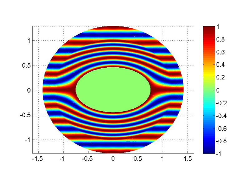
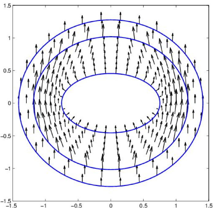
Figure 8. Real part of the electric-field distribution (left) and the related Poynting vector (right), where the incident angle $\theta_{0}={\pi}$.

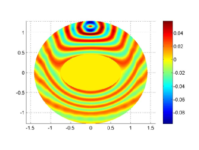
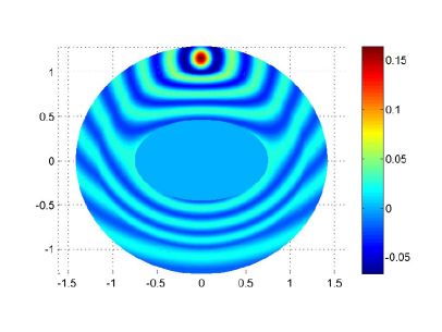
Figure 9. The real (left) and imaginary (right) part of electric-field distribution with different sources.

Concluding remarks

From a new perspective, we proposed CBCs for the ideal circular and elliptic cylindrical cloaks, which, together with a super-accurate spectral-element solver, demonstrated that the cloaks can achieve perfect concealment of incoming incident waves with very mild conditions on the incident frequency. We also illustrated the perfect cloaking effect, when the incoming wave is generated by a source exterior to the cloaking device.

The idea and approach in this paper can shed light on the study of, e.g., polygonal cloaks [15, 60, 39], and can lead to appropriate CBCs for time-domain simulations [23, 33].

Acknowledgment The authors would like to thank Professor Jichun Li from University of Nevada, Las Vegas, USA, and Professors Baile Zhang and Handong Sun in the Division of Physics and Applied Physics of Nanyang Technological University, for fruitful discussions.

Appendix A Proof of Proposition $2.2$

It is clear that by (35),

$${\rm Re}\big{\{}{\mathcal{B}}_{m}(\hat{u}_{m},\hat{u}_{m})\big{\}}=\|\hat{u}_{m}^{\prime}\|_{\omega}^{2}+m^{2}\|\hat{u}_{m}\|_{\omega^{-1}}^{2}-k^{2}\|\rho\hat{u}_{m}\|^{2}_{\omega}-R_{3}\,{\rm Re}(\mathcal{T}_{m,k})|\hat{u}_{m}(R_{3})|^{2},$$ (A.88)

and

$${\rm Im}\big{\{}{\mathcal{B}}_{m}(\hat{u}_{m},\hat{u}_{m})\big{\}}=-R_{3}\,{\rm Im}(\mathcal{T}_{m,k})|\hat{u}_{m}(R_{3})|^{2}.$$ (A.89)

Recall that (see, e.g., [45, 53]):

$${\rm Re}(\mathcal{T}_{m,k})<0,\quad{\rm Im}(\mathcal{T}_{m,k})>0.$$ (A.90)

Thus, we have

$${\rm Re}\big{\{}{\mathcal{B}}_{m}(\hat{u}_{m},\hat{u}_{m})\big{\}}\geq\|\hat{u}_{m}^{\prime}\|_{\omega}^{2}+m^{2}\|\hat{u}_{m}\|_{\omega^{-1}}^{2}-k^{2}\|\rho\hat{u}_{m}\|^{2}_{\omega},$$ (A.91)

and $\hat{u}_{m}(R_{3})=0,$ if $\hat{g}_{m}=0.$ Using the Fredholm alternative (cf. [45, Thm. 5.4.5]), we reach the conclusion.

Appendix B Proof of Proposition $3.2$

For simplicity, denote

$${\rm M}_{m}^{(i)}={\rm Mc}_{m}^{(i)}\;\;{\rm or}\;\;{\rm Ms}_{m}^{(i)},\quad i=1,2,3;\quad{\mathcal{D}}_{m}={\mathcal{D}}_{m}^{\rm c}\;\;{\rm or}\;\;{\mathcal{D}}_{m}^{\rm s}.$$

Recall that (see e.g., [1])

$${\rm M}_{m}^{(3)}:={\rm M}_{m}^{(1)}+{\rm i}{\rm M}_{m}^{(2)};\quad{\rm M}_{m}^{(1)}{{\rm M}_{m}^{(2)}}^{\prime}-{\rm M}_{m}^{(2)}{{\rm M}_{m}^{(1)}}^{\prime}=\frac{2}{\pi}\,.$$ (B.92)

Then a direct calculation from (72) and (B.92) leads to

$${\rm Im}({\mathcal{D}}_{m})=\frac{{\rm M}_{m}^{(1)}(\xi_{3};q){{\rm M}_{m}^{(2)}}^{\prime}(\xi_{3};q)-{\rm M}_{m}^{(2)}(\xi_{3};q){{\rm M}_{m}^{(1)}}^{\prime}(\xi_{3};q)}{|{\rm M}_{m}^{(3)}(\xi_{3};q)|^{2}}=\frac{2/\pi}{|{\rm M}_{m}^{(3)}(\xi_{3};q)|^{2}}>0.$$ (B.93)

Moreover, by (71d),

$${\rm Re}({\mathcal{D}}_{m})=\frac{{\rm M}_{m}^{(1)}(\xi_{3};q){{\rm M}_{m}^{(1)}}^{\prime}(\xi_{3};q)+{\rm M}_{m}^{(2)}(\xi_{3};q){{\rm M}_{m}^{(2)}}^{\prime}(\xi_{3};q)}{|{\rm M}_{m}^{(3)}(\xi_{3};q)|^{2}},$$ (B.94)

Note that $\{{\rm M}_{m}^{(i)}(\xi;q)\}_{i=1}^{2}$ can not have common zero, and are analytic for all $\xi>0$ (see, e.g., [1]), so $|{\rm Re}({\mathcal{D}}_{m})|$ is a finite constant for fixed $m,q$ and $\xi_{3}.$ To this end, let $C$ be a generic positive constant depending on $m,q,\xi_{2}$ and $\xi_{3}.$

We first consider (74) and obtain that

$${\rm Re}\big{\{}{\mathcal{B}}_{m}^{\rm c}(\hat{v}_{m}^{\rm c},\hat{v}_{m}^{\rm c})\big{\}}=\|\varpi(\hat{v}_{m}^{\rm c})^{\prime}\|^{2}+\tilde{\lambda}_{m}^{\rm c}\|\varpi^{-1}\hat{v}_{m}^{\rm c}\|^{2}-4q\|\varpi^{-1}{\chi}\hat{v}_{m}^{\rm c}\|^{2}-{\rm Re}({\mathcal{D}}_{m}^{\rm c})|\hat{v}_{m}^{\rm c}(\xi_{3})|^{2},$$ (B.95)

and

$${\rm Im}\big{\{}{\mathcal{B}}_{m}^{\rm c}(\hat{v}_{m}^{\rm c},\hat{v}_{m}^{\rm c})\big{\}}=-{\rm Im}({\mathcal{D}}_{m}^{\rm c})|\hat{v}_{m}^{\rm c}(\xi_{3})|^{2}.$$ (B.96)

Let $I_{2}=(\xi_{2},\xi_{3})$ as before. Recall the Sobolev inequality (see, e.g., [51, (B.33)]): for any $w\in H^{1}(I_{2}),$

$$\max_{x\in\bar{I}_{2}}|w(x)|^{2}\leq\Big{(}\frac{1}{\xi_{3}-\xi_{2}}+2\Big{)}\|w\|_{L^{2}(I_{2})}\|w\|_{H^{1}(I_{2})}.$$ (B.97)

Therefore, we further derive from the Cauchy-Schwartz inequality that

$$\begin{split}|{\rm Re}({\mathcal{D}}_{m}^{\rm c})|&|\hat{v}_{m}^{\rm c}(\xi_{3})|^{2}\leq C\big{(}\|\varpi(\hat{v}_{m}^{\rm c})^{\prime}\|^{2}+\|\chi\hat{v}_{m}^{\rm c}\|^{2}\big{)}^{{1}/{2}}\|\chi\hat{v}_{m}^{\rm c}\|\\ &\leq C\big{(}\|\varpi(\hat{v}_{m}^{\rm c})^{\prime}\|\|\chi\hat{v}_{m}^{\rm c}\|+\|\chi\hat{v}_{m}^{\rm c}\|^{2}\big{)}\leq\frac{1}{2}\|\varpi(\hat{v}_{m}^{\rm c})^{\prime}\|^{2}+C\|\chi\hat{v}_{m}^{\rm c}\|^{2}.\end{split}$$ (B.98)

Therefore, by (B.95) and (B.98),

$${\rm Re}\big{\{}{\mathcal{B}}_{m}^{\rm c}(\hat{v}_{m}^{\rm c},\hat{v}_{m}^{\rm c})\big{\}}\geq\frac{1}{2}\|\varpi(\hat{v}_{m}^{\rm c})^{\prime}\|^{2}+\tilde{\lambda}_{m}^{\rm c}\|\varpi^{-1}\hat{v}_{m}^{\rm c}\|^{2}-(4q+C)\|\varpi^{-1}{\chi}\hat{v}_{m}^{\rm c}\|^{2}.$$ (B.99)

Moreover, by (B.93), $\hat{v}_{m}^{\rm c}(\xi_{3})=0,$ if $\hat{\phi}_{m}^{\rm c}=0.$ Using the Fredholm alternative (see, e.g., [45, Thm. 5.4.5]), we reach the conclusion.

The uniqueness of the solution for (75) can be shown similarly.

References

- [1] M. Abramowitz and I.A. Stegun, editors. Handbook of Mathematical Functions with Formulas, Graphs, and Mathematical Tables. A Wiley-Interscience Publication. John Wiley & Sons Inc., New York, 1984. Reprint of the 1972 edition, Selected Government Publications.
- [2] R.A. Adams and J.J. Fournier. Sobolev Spaces, volume 140. Academic press, 2003.
- [3] M.A. Al-Gwaiz. Sturm-Liouville Theory and Its Applications. Springer Undergraduate Mathematics Series. Springer-Verlag London, Ltd., London, 2008.
- [4] H. Ammari, H. Kang, H. Lee, M. Lim, and S. Yu. Enhancement of near cloaking for the full Maxwell equations. SIAM J. Appl. Math., 73(6):2055–2076, 2013.
- [5] J.P. Berenger. A perfectly matched layer for the absorption of electromagnetic waves. J. Comput. Phys., 114(2):185–200, 1994.
- [6] J.P. Boyd. Chebyshev and Fourier Spectral Methods. Dover Publications, second edition, 2001.
- [7] W.S. Cai and V.M. Shalaev. Optical Metamaterials, volume 10. Springer, 2010.
- [8] H.Y. Chen. Transformation optics in orthogonal coordinates. J. Opt. A: Pure Appl. Opt., 11(7):75–102, 2009.
- [9] H.Y. Chen, C.T. Chan, and P. Sheng. Transformation optics and metamaterials. Nature Materials, 9(5):387–396, 2010.
- [10] E. Cojocaru. Exact analytical approaches for elliptic cylindrical invisibility cloaks. J. Opt. Soc. Am. B., 26(5):1119–1128, 2009.
- [11] R. Courant and D. Hilbert. Methods of Mathematical Physics. Vol. I. Interscience Publishers, Inc., New York, N.Y., 1953.
- [12] T.J. Cui, D.R. Smith, and R.P. Liu. Metamaterials: Theory, Design, and Applications. Springer, 2009.
- [13] S. Cummer, B. Popa, D. Schurig, D. Smith, and J. Pendry. Full-wave simulations of electromagnetic cloaking structures. Phys. Rev. E, 74(3):036621, 2006.
- [14] Kown D.H. Transformation electromagnetics and optics. Forum for Electromagnetic Research Methods and Application Technologies (FERMAT), 1(8):1–11, 2014.
- [15] A. Diatta, A. Nicolet, S. Guenneau, and F. Zolla. Tessellated and stellated invisibility. Optics Express, 17(16):13389–13394, 2009.
- [16] Q. Fang, D.P. Nicholls, and J. Shen. A stable, high–order method for two–dimensional bounded–obstacle scattering. J. Comput. Phys., 224:1145–1169, 2007.
- [17] Q. Fang, J. Shen, and L.L. Wang. An efficient and accurate spectral method for acoustic scattering in elliptic domains. Numer. Math.: Theory, Methods Appl., 2:258–274, 2009.
- [18] R. Fleury and A. Alù. Cloaking and invisibility: A review. Forum for Electromagnetic Research Methods and Application Technologies (FERMAT), 1(7):1–24, 2014.
- [19] D. Gottlieb and S.A. Orszag. Numerical Analysis of Spectral Methods: Theory and Applications. SIAM-CBMS, Philadelphia, 1977.
- [20] A. Greenleaf, Y. Kurylev, M. Lassas, and G. Uhlmann. Cloaking devices, electromagnetic wormholes, and transformation optics. SIAM Review, 51(1):3–33, 2009.
- [21] A. Greenleaf, M. Lassas, and G. Uhlmann. On nonuniqueness for Calderon’s inverse problem. Math. Res. Lett., 10(5/6):685–694, 2003.
- [22] M.J. Grote and J.B. Keller. On non-reflecting boundary conditions. J. Comput. Phys., 122:231–243, 1995.
- [23] Y. Hao and R. Mittra. FDTD Modeling of Metamaterials: Theory and Applications. Artech House, 2008.
- [24] Y.Y. Ji, H. Wu, H.P. Ma, and B.Y. Guo. Multidomain pseudospectral methods for nonlinear convection-diffusion equations. Appl. Math. Mech. (English Ed.), 32(10):1255–1268, 2011.
- [25] W.X. Jiang, T.J. Cui, G.X. Yu, X.Q. Lin, Q. Cheng, and J.Y. Chin. Arbitrarily elliptical–cylindrical invisible cloaking. J. Phys. D: Appl. Phys., 41(8):085504, 2008.
- [26] R.V. Kohn, D. Onofrei, M.S. Vogelius, and M.I. Weinstein. Cloaking via change of variables for the Helmholtz equation. Comm. Pure Appl. Math., 63(8):973–1016, 2010.
- [27] D.H. Kwon and D.H. Werner. Two-dimensional eccentric elliptic electromagnetic cloaks. Appl. Phys. Lett, 92(1):013505, 2008.
- [28] M. Lassas and T. Zhou. Singular partial differential operators and pseudo-differential boundary conditions in invisibility cloaking. In Fourier Analysis, Trends in Mathematics, pages 263–284, 2014. Springer, Switzerland.
- [29] M. Lassas and T. Zhou. Two dimensional invisibility cloaking for Helmholtz equation and non-local boundary conditions. Math. Res. Lett., 18(3):473–488, 2011.
- [30] U. Leonhardt. Optical conformal mapping. Science, 312(5781):1777–1780, 2006.
- [31] U. Leonhardt and T. Philbin. Geometry and Light: The Science of Invisibility. Dover Publications, 2012.
- [32] J.C. Li and Y.Q. Huang. Mathematical simulation of cloaking metamaterial structures. Adv. Appl. Math. Mech, 4:93–101, 2012.
- [33] J.C. Li and Y.Q. Huang. Time-Domain Finite Element Methods for Maxwell’s Equations in Metamaterials, volume 43. Springer, 2012.
- [34] J.C. Li, Y.Q. Huang, and W. Yang. Developing a time-domain finite-element method for modeling of electromagnetic cylindrical cloaks. J. Comput. Phys., 231(7):2880–2891, 2012.
- [35] J.C. Li, Y.Q. Huang, and W. Yang. Well-posedness study and finite element simulation of time-domain cylindrical and elliptical cloaks. Math. Comp., In press, 2014.
- [36] J.Z. Li, H.Y. Liu, and H.P. Sun. Enhanced approximate cloaking by SH and FSH lining. Inverse Problems, 28(7):075011, 2012.
- [37] H.Y. Liu and H.P. Sun. Enhanced near-cloak by FSH lining. J. Math. Pures Appl., 99(1):17–42, 2013.
- [38] H.Y. Liu and T. Zhou. On approximate electromagnetic cloaking by transformation media. SIAM J. Appl. Math., 71(1):218–241, 2011.
- [39] Y. Luo, L.X. He, S.Z. Zhu, and Y. Wang. Arbitrary polygonal cloaks with multiple invisible regions. J. Modern Opt., 58(1):14–20, 2011.
- [40] H. Ma, S.B. Qu, Z. Xu, J.Q. Zhang, B.W. Chen, and J.F. Wang. Material parameter equation for elliptical cylindrical cloaks. Phys. Rev. A, 77(1):013825, 2008.
- [41] N.W. McLachlan. Theory and Application of Mathieu Functions, volume 4. Dover New York, 1964.
- [42] F.P. Mechel. Formulas of Acoustics, volume 2. Springer, 2002.
- [43] P. Monk. Finite Element Methods for Maxwell’s Equations. Numerical Mathematics and Scientific Computation. Oxford University Press, New York, 2003.
- [44] J.C. Nédélec. Mixed finite elements in . Numer. Math., 35(3):315–341, 1980.
- [45] J.C. Nédélec. Acoustic and Electromagnetic Equations, volume 144 of Applied Mathematical Sciences. Springer-Verlag, New York, 2001. Integral representations for harmonic problems.
- [46] S.J. Orfanidis. Electromagnetic Waves and Antennas. Rutgers University, 2002.
- [47] J. B. Pendry, D. Schurig, and D. R. Smith. Controlling electromagnetic fields. Science, 312(5781):1780–1782, 2006.
- [48] Z. Ruan, M. Yan, C.W. Neff, and M. Qiu. Ideal cylindrical cloak: perfect but sensitive to tiny perturbations. Phys. Rev. Lett., 99(11):113903, 2007.
- [49] D. Schurig, J. Mock, B. Justice, S. Cummer, J. Pendry, A. Starr, and D. Smith. Metamaterial electromagnetic cloak at microwave frequencies. Science, 314(5801):977–980, 2006.
- [50] J. Shen. Efficient spectral-Galerkin methods III. polar and cylindrical geometries. SIAM J. Sci. Comput., 18:1583–1604, 1997.
- [51] J. Shen, T. Tang, and L.L. Wang. Spectral Methods: Algorithms, Analysis and Applications, volume 41 of Springer Series in Computational Mathematics. Springer-Verlag, Berlin, Heidelberg, 2011.
- [52] J. Shen and L.L. Wang. Spectral approximation of the Helmholtz equation with high wave numbers. SIAM J. Numer. Anal., 43(2):623–644, 2005.
- [53] J. Shen and L.L. Wang. Analysis of a spectral-Galerkin approximation to the Helmholtz equation in exterior domains. SIAM J. Numer. Anal., 45(5):1954–1978, 2007.
- [54] J. Shen, L.L. Wang, and H.Y. Li. A triangular spectral element method using fully tensorial rational basis functions. SIAM J. Numer. Anal., 47(3):1619–1650, 2009.
- [55] L.L. Wang, B. Wang, and X.D. Zhao. Fast and accurate computation of time-domain acoustic scattering problems with exact nonreflecting boundary conditions. SIAM J. Appl. Math., 72(6):1869–1898, 2012.
- [56] G.N. Watson. A Treatise of the Theory of Bessel Functions (second edition). Cambridge University Press, Cambridge, UK, 1966.
- [57] R. Weder. The boundary conditions for point transformed electromagnetic invisibility cloaks. J. Phys. A: Math. Theor., 41(41):415401, 2008.
- [58] D.H. Werner and D.H. Kwon. Transformation Electromagnetics and Metamaterials: Fundamental Principles and Applications. Springer, 2014.
- [59] E.T. Whittaker and G.N. Watson. A Course of Modern Analysis. Cambridge university press, 1927.
- [60] Q. Wu, K. Zhang, F.Y. Meng, and L.W. Li. Material parameters characterization for arbitrary -sided regular polygonal invisible cloak. J. Phys. D: Appl. Phys., 42(3):035408, 2009.
- [61] B.L. Zhang. Electrodynamics of transformation-based invisibility cloaking. Light: Science & Applications, 1(10):e32, 2012.
- [62] B.L. Zhang, H.S. Chen, B. Wu, Y. Luo, L. Ran, and J.A. Kong. Response of a cylindrical invisibility cloak to electromagnetic waves. Phys. Rev. B, 76(12):121101, 2007.
- [63] F. Zolla, S. Guenneau, A. Nicolet, and J.B. Pendry. Electromagnetic analysis of cylindrical invisibility cloaks and the mirage effect. Optics Letters, 32(9):1069–1071, 2007.