Abstract

We enlighten relations between the Källén function, allowing in a simple way to distinguish between virtual and real processes involving massive particles, and the dilogarithms occurring as results of loop calculations for such kind of processes.

1 Introduction

The name of the swedish physicist and one of the founders of the CERN, early deceased Anders Olof Gunnar Källén (1926–1968), is related forever to three-particle vertices connecting particles of different masses. As an example one can use the decay process of the top quark into a bottom quark and a $W$ boson, with $91\%$ the main decay channel of the top quark seen at the LHC [1]. Using as a reference frame the rest frame of the top quark, the kinematics of

$$t(p_{t})\to b(p_{b})+W^{+}(p_{W})$$ (1)

can easily be calculated as a warm-up exercise. From four-momentum conservation one obtains $\vec{p}_{b}+\vec{p}_{W}=\vec{0}$ and $E_{b}+E_{W}=m_{t}$. The on-shell conditions for the two produced particles read

$$m_{b}^{2}=E_{b}^{2}-\vec{p}_{b}^{2},\qquad m_{W}^{2}=E_{W}^{2}-\vec{p}_{W}^{2}.$$ (2)

Inserting $E_{W}=m_{t}-E_{b}$ into the last equation, using $\vec{p}_{W}^{2}=\vec{p}_{b}^{2}$ and solving for $E_{b}$ one obtains

$$E_{b}=\frac{m_{t}^{2}+m_{b}^{2}-m_{W}^{2}}{2m_{t}},\quad\mbox{likewise}\quad E_{W}=\frac{m_{t}^{2}-m_{b}^{2}+m_{W}^{2}}{2m_{t}}.$$ (3)

Finally,

$$\vec{p}_{b}^{2}=E_{b}^{2}-m_{b}^{2}=\frac{(m_{t}^{2}+m_{b}^{2}-m_{W}^{2})^{2}-4m_{t}^{2}m_{b}^{2}}{4m_{t}^{2}}=\frac{\lambda(m_{t}^{2},m_{b}^{2},m_{W}^{2})}{4m_{t}^{2}}$$ (4)

where the only mixed product $2m_{t}^{2}m_{b}^{2}$ changes sign, leading to the totally symmetric Källén function

$$\lambda(a,b,c):=a^{2}+b^{2}+c^{2}-2ab-2ac-2bc.$$ (5)

Therefore,

$$|\vec{p}_{b}|=|\vec{p}_{W}|=\frac{\sqrt{\lambda(m_{t}^{2},m_{b}^{2},m_{W}^{2})}}{2m_{t}}.$$ (6)

As will be shown in Sec. 1 of this paper, the Källén function appears in different kinematic situations, though describing always the same relation, namely the realness respectively virtualness of processes involving three (massive) particles. Parallels to symmetries for dilogarithms are shown in Sec. 2. Finally, in Sec. 3 we give our conclusions.

1.1 The Källén triangle

Looking more closely at the Källén function $\lambda(m_{1}^{2},m_{2}^{2},m_{3}^{2})$ of three particles with masses $m_{1}$, $m_{2}$ and $m_{3}$, the analytic behaviour unfolds a rich spectrum of real and virtual processes. The function is zero for any one of the thresholds

$$m_{1}^{2}=(m_{2}\pm m_{3})^{2},\qquad m_{2}^{2}=(m_{3}\pm m_{1})^{2},\qquad m_{3}^{2}=(m_{1}\pm m_{2})^{2}.$$ (7)

Allowing only positive values for the three masses, in the $(m_{1},m_{2},m_{3})$ phase space the zeros of the Källén function are located on the three planes spanned by each two of the three face diagonals $m_{1}=m_{2}$, $m_{1}=m_{3}$ and $m_{2}=m_{3}$. Up to the general normalization one can visualise the phase space by cutting the first octant by a plane orthogonal to the space diagonal. On this plane the first octant will appear as upright equilateral domain triangle (cf. Fig. 1), the corners representing the $m_{i}$ axes, and the opposite sides representing the coordinate planes $m_{i}=0$. The zeros of the Källén function are found on the three lines connecting the midpoints of the sides of the triangle (cf. Fig. 2). The equilateral triangle enclosed by these three lines is called the Källén triangle. While this triangle is the region where the Källén function becomes negative, the other three triangles are regions with positive Källén function, each of them containing a coordinate axis. Special values are

$$\lambda(m_{1}^{2},m_{1}^{2},m_{1}^{2}) = -3m_{1}^{4}\qquad\mbox{(center)},$$

$$\lambda(m_{1}^{2},m_{2}^{2},m_{2}^{2}) = m_{1}^{4}-4m_{1}^{2}m_{2}^{2}\qquad\mbox{(medians)},$$

$$\lambda(m_{1}^{2},m_{2}^{2},0) = (m_{1}^{2}-m_{2}^{2})^{2}\qquad\mbox{(sides)},$$

$$\lambda(m_{1}^{2},0,0) = m_{1}^{4}\qquad\mbox{(corners)}.$$ (8)

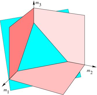
Figure 1: Construction of the domain triangle of the first octant $m_{i}\geq 0$ ($i=1,2,3$)

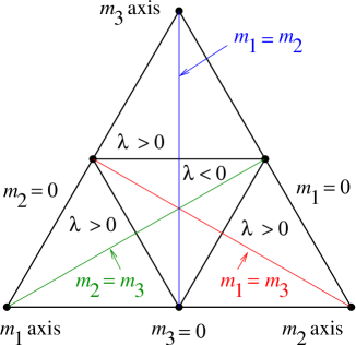
Figure 2: Regions of positive and negative Källén function $\lambda=\lambda(m_{1}^{2},m_{2}^{2},m_{3}^{2})$. The axes of the three-dimensional phase space are represented by the corners of the domain triangle. The innermost triangle (with $\lambda<0$) is called the Källén triangle throughout this paper.

A negative value of the Källén function means that the sum of two of the masses is larger than the third one. This means physically that none of the three particles can decay into the other two. The process is a virtual one, leaving at least one of the particles off-shell, i.e. with a momentum squared which is smaller than the squared mass of this particle. On the other hand, a positive Källén function means that exactly one decay channel is real. Taking for instance the region connected to the $m_{1}$ axis, all points in the lower left triangle in Fig. 2 represent possible decays through the channel $1\to 2+3$ because $m_{1}$ is larger than the sum $m_{2}+m_{3}$. Therefore, one can conclude that the triangle in Fig. 2 gives structure and direction to processes involving three massive particles.

1.2 Cascade processes

Usually, three-particle interactions appear within a more complicated process. In this case the masses are (partially) replaced by invariant squared momenta $k_{i}^{2}$. On tree level such a process is a cascade process as explained for instance in Refs. [2, 3]. For a cascade process including $n$ final particles with masses $m_{i}$ ($i=1,2,\ldots,n$), the $n$-particle phase space

$$\Phi_{n}(p;m_{1}^{2},m_{2}^{2},\ldots,m_{n}^{2})=\int\prod_{i=1}^{n}\frac{d^{4}p_{i}}{(2\pi)^{4}}\left(2\pi\delta(p_{i}^{2}-m_{i}^{2})\right)(2\pi)^{4}\delta^{(4)}(p-\sum_{i=1}^{n}p_{i})$$ (9)

can be factorized. Given for instance the momentum $p_{1}$ of the first particle emitted from this process, the remaining momentum $k_{1}=p-p_{1}$ is mediated by a virtual particle. One can define an invariant mass $M$ with $M^{2}=k_{1}^{2}$ with the only condition that $k_{1}$ is time-like. Separating the first phase space integration from the other ones and inserting the trivial identities

$$1=\int\frac{dM^{2}}{2\pi}2\pi\delta(k_{1}^{2}-M^{2}),\qquad 1=\int\frac{d^{4}k_{1}}{(2\pi)^{4}}(2\pi)^{4}\delta^{(4)}(p-p_{1}-k_{1})$$ (10)

one obtains [3]

$$\Phi_{n}(p;m_{1}^{2},m_{2}^{2},\ldots,m_{n}^{2})=\int\frac{dk_{1}^{2}}{2\pi}\Phi_{2}(p;m_{1}^{2},k_{1}^{2})\Phi_{n-1}(k_{1};m_{2}^{2},\ldots,m_{n}^{2}).$$ (11)

As an example we consider the cascade decay $t\to b+W^{+}(\to c+\bar{s})$. The first part $\Phi_{2}(p;m_{1}^{2},k_{1}^{2})$ of the cascade phase space is given by the phase space

$$\Phi_{2}(p_{t};m_{b}^{2},m_{W}^{2})=\frac{|\vec{p}_{W}|}{4m_{t}(2\pi)^{2}}\int d\Omega_{W}=\frac{\sqrt{\lambda(m_{t}^{2},m_{b}^{2},m_{W}^{2})}}{8m_{t}^{2}(2\pi)^{2}}\int d\Omega_{W}$$ (12)

of the previous (simpler) process $t\to b+W^{+}$ where $m_{W}^{2}$ is replaced by $k_{1}^{2}=p_{W}^{2}$. For the second part $\Phi_{2}(k_{1};m_{2}^{2},m_{3}^{2})$ one obtains in a similar manner

$$\Phi_{2}(p_{W};m_{c}^{2},m_{s}^{2})=\frac{\sqrt{\lambda(p_{W}^{2},m_{c}^{2},m_{s}^{2})}}{8p_{W}^{2}(2\pi)^{2}}\int d\Omega_{c}.$$ (13)

Assuming that one can perform the solid angle integrations for the $W$ boson ($\Omega_{W}=4\pi$) and for the $c$ quark ($\Omega_{c}=4\pi$) trivially, one is left with the three-particle phase space

$$\Phi_{3}(p_{t};m_{b}^{2},m_{c}^{2},m_{s}^{2})=\int\frac{dp_{W}^{2}}{2\pi}\frac{\sqrt{\lambda(m_{t}^{2},m_{b}^{2},p_{W}^{2})}}{8m_{t}^{2}(2\pi)^{2}}\frac{\sqrt{\lambda(p_{W}^{2},m_{c}^{2},m_{s}^{2})}}{8p_{W}^{2}(2\pi)^{2}}(4\pi)^{2}.$$ (14)

1.3 Limits for the phase space

The example just introduced is an ideal playground for the implications caused by the Källén functions in case of integrations over inner lines. Even though the intermediate $W$ boson can be off-shell, the phase space has to be real. Therefore, the two conditions

$$\lambda(m_{t}^{2},m_{b}^{2},p_{W}^{2}) = ((m_{t}-m_{b})^{2}-p_{W}^{2})((m_{t}+m_{b})^{2}-p_{W}^{2})\ \geq\ 0,$$ (15)

$$\lambda(p_{W}^{2},m_{c}^{2},m_{s}^{2}) = (p_{W}^{2}-(m_{c}-m_{s})^{2})(p_{W}^{2}-(m_{c}+m_{s})^{2})\ \geq\ 0$$ (16)

determine the phase space region for $p_{W}^{2}$ and at the same time an appropriate substitution to calculate the integral analytically. Taking into account the known quark mass hierarchy, the two conditions result in

$$(m_{c}+m_{s})^{2}\leq p_{W}^{2}\leq(m_{t}-m_{b})^{2}.$$ (17)

1.4 An appropriate substitution

Neglecting the masses of $c$ and $s$ quarks, the phase space simplifies to

$$\Phi_{3}(p_{t};m_{b}^{2},0,0)=\frac{1}{512\pi^{3}m_{t}^{2}}\int_{0}^{(m_{t}-m_{b})^{2}}\sqrt{\lambda(m_{t}^{2},m_{b}^{2},p_{W}^{2})}dp_{W}^{2}.$$ (18)

The square root in Eq. (18) can be simplified by choosing one of the factors in Eq. (15) as new variable, e.g. $z^{\prime}=(m_{t}-m_{b})^{2}-p_{W}^{2}$. The second factor is then given by

$$(m_{t}+m_{b})^{2}-p_{W}^{2}=(m_{t}+m_{b})^{2}-(m_{t}-m_{b})^{2}+z^{\prime}=4m_{t}m_{b}+z^{\prime},$$ (19)

and the upper limit is given by $z^{\prime}=0$. However, $z^{\prime}$ is not the optimal choice. Using instead $z=z^{\prime}+2m_{t}m_{b}=m_{t}^{2}+m_{b}^{2}-p_{W}^{2}$ the square root simplifies to

$$\sqrt{\lambda(m_{t}^{2},m_{b}^{2},p_{W}^{2})}=\sqrt{z^{2}-4m_{t}^{2}m_{b}^{2}}.$$ (20)

The integration can be performed by using $z=2m_{t}m_{b}\cosh\zeta$,

$$\Phi(p_{t};m_{b}^{2},0,0)=\frac{1}{512\pi^{3}m_{t}^{2}}\int_{2m_{t}m_{b}}^{m_{t}^{2}+m_{b}^{2}}\sqrt{z^{2}-4m_{t}^{2}m_{b}^{2}}dz=\frac{m_{b}^{2}}{128\pi^{2}}\int_{0}^{\zeta_{0}}\sinh^{2}\zeta\,d\zeta$$ (21)

where

$$\zeta_{0}=\mathop{\rm arcosh}\nolimits\left(\frac{m_{t}^{2}+m_{b}^{2}}{2m_{t}m_{b}}\right)=\ln\left(\frac{m_{t}}{m_{b}}\right).$$ (22)

Finally, one can use $t=m_{b}^{2}e^{2\zeta}$ to obtain

$$\Phi(p_{t};m_{b}^{2},0,0)=\frac{1}{128\pi^{2}}\int_{m_{b}^{2}}^{m_{t}^{2}}\frac{(t-m_{b}^{2})^{2}}{8t^{2}}dt.$$ (23)

1.5 Lorentz boosts

To conclude this section, let us dwell on the parameter $\zeta$ used in the substitution. This parameter is related to the masses and the invariant momentum square by

$$\cosh\zeta=\frac{m_{t}^{2}+m_{b}^{2}-p_{W}^{2}}{2m_{t}m_{b}},\qquad\sinh\zeta=\frac{\sqrt{\lambda(m_{t}^{2},m_{b}^{2},p_{W}^{2})}}{2m_{t}m_{b}}.$$ (24)

Comparing with Eqs. (3) and (6) one realizes that $\zeta$ is the rapidity for the transition between the $t$ and $b$ quark rest frames, the exponential representation being

$$e^{\pm\zeta}=\frac{m_{t}^{2}+m_{b}^{2}-p_{W}^{2}\pm\sqrt{\lambda(m_{t}^{2},m_{b}^{2},p_{W}^{2})}}{2m_{t}m_{b}}.$$ (25)

2 Dilogarithms

Dilogarithms appear in two-fold integrations where the pole of the integrand is shifted (or in similar arrangements related to this one by the shuffle algebra [4]). Such a shift is usually due to the occurence of mass contributions. This is the reason why the arguments of the dilogarithms and their relation to the mass configuration described by the Källén function is investigated in this section. The “classical” dilogarithm is given by the integral representation

$$\mathop{\rm Li}\nolimits_{2}(z):=-\int_{0}^{z}\frac{dz^{\prime}}{z^{\prime}}\ln(1-z^{\prime}).$$ (26)

The classical dilogarithm is a special case of a polylogarithm and is an analytical function in the whole complex plane except for the interval $[1,\infty]$ along the positive real axis where the branch cut is located. Starting from the branch point at $z=1$, the branch cut separates two different Riemannian sheets of the multi-valued function. There are two one-parameter and a couple of two- and three-parameter identities that allow to relate dilogarithms with different arguments [5, 6, 7, 8, 9]. The two one-parameter identities are given by [5]

$$\mathop{\rm Li}\nolimits_{2}(z)+\mathop{\rm Li}\nolimits_{2}\left(\frac{1}{z}\right) = -\frac{\pi^{2}}{6}-\frac{1}{2}\ln^{2}(-z),\qquad z\not\in[0,1[$$ (27)

$$\mathop{\rm Li}\nolimits_{2}(z)+\mathop{\rm Li}\nolimits_{2}(1-z) = \frac{\pi^{2}}{6}-\ln z\ln(1-z).$$ (28)

An additional useful identity is

$$\mathop{\rm Li}\nolimits_{2}(z)+\mathop{\rm Li}\nolimits_{2}(-z)=\frac{1}{2}\mathop{\rm Li}\nolimits_{2}(z^{2}).$$ (29)

2.1 The hexagon orbit

For the arguments of the dilogarithms the two identities (27) and (28) are involutions. Because of this, one can create a closed chain of transitions for the argument which constitutes a hexagon,

$$z$$

(30)

For real-valued arguments this transition orbit helps to constrain the argument to a value lower or equal to $1$, gaining a real value for the dilogarithm. A pragmatic argument can be very helpful to choose an appropriate hexagon orbit transition: processes including only real particles have to lead to real phase space integrals. Therefore, a negative argument for the logarithms obtained together with the dilogarithm in calculations like

$$\int\ln(\alpha z+\beta)\frac{dz}{z}=-\mathop{\rm Li}\nolimits_{2}\left(-\frac{\alpha}{\beta}z\right)+\ln\beta\,\ln z+C$$ (31)

indicate that the argument of the dilogarithm still is not in an appropriate form.

2.2 The Bloch–Wigner dilogarithm

A similar orbit, though for complex arguments, is given in Refs. [6, 7, 8, 9] for the Bloch–Wigner dilogarithm

$$D(z)=\mathop{\rm Im}\nolimits\left(\mathop{\rm Li}\nolimits_{2}(z)+\ln|z|\ln(1-z)\right)$$ (32)

which is mainly (i.e. up to a double-logarithmic correction) the imaginary part of the classical dilogarithm. The identities, induced by the two involutions, are given by

$$D(z)=-D(z^{-1})=D(1-z^{-1})=-D(-z(1-z)^{-1})=D((1-z)^{-1})=-D(1-z)$$ (33)

and $D(\bar{z})=-D(z)$. In Ref. [9] these identities are applied to the (complex) root

$$z(m_{1}^{2},m_{2}^{2},m_{3}^{2})=\frac{m_{1}^{2}-m_{2}^{2}+m_{3}^{2}+\sqrt{\lambda(m_{1}^{2},m_{2}^{2},m_{3}^{2})}}{2m_{1}^{2}}$$ (34)

where the discriminant $\lambda(m_{1}^{2},m_{2}^{2},m_{3}^{2})$ is again the Källén function, assumed to be negative. An orbit with constant value for $D$ given by

$$D(z)=D(\bar{z}^{-1})=D(1-z^{-1})=D(-\bar{z}(1-\bar{z})^{-1})=D((1-z)^{-1})=D(1-\bar{z})$$ (35)

is obtained by combining the two involutions with a third one, namely the calculation of the complex conjugate. As mentioned in Ref. [9], the points of the orbit can be obtained from the starting point $z(m_{1}^{2},m_{2}^{2},m_{3}^{2})$ by interchanging the squared masses $m_{1}^{2}$, $m_{2}^{2}$ and $m_{3}^{2}$. This invariance describes a symmetry of the Bloch–Wigner dilogarithm which is manifest already for the Källén function. In the following we compare these two functions.

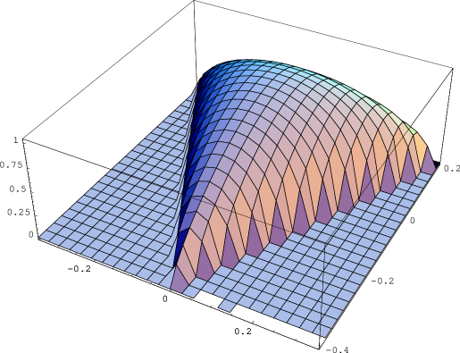
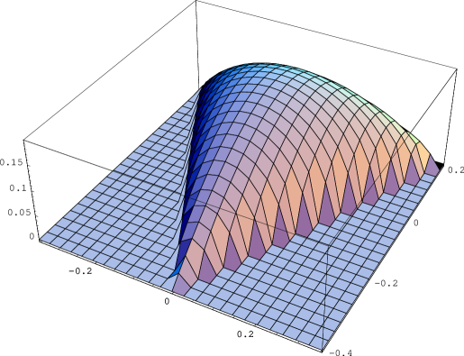
Figure 3: Topography of $D(z(m_{1}^{2},m_{2}^{2},m_{3}^{2}))$, $z(m_{1}^{2},m_{2}^{2},m_{3}^{2})$ taken from Eq. (34) (top), and $\mathop{\rm Im}\nolimits(\sqrt{\lambda(m_{1}^{2},m_{2}^{2},m_{3}^{2})})$ (bottom) over the Källén triangle

2.3 Support and similarities

Because the Bloch–Wigner dilogarithm $D(z)$ vanishes for real values of $z$, it is evident from Eq. (34) that it vanishes for positive values of the Källén function. Therefore, the support of the Bloch–Wigner dilogarithm and the Källén function within the domain triangle are both given by the Källén triangle shown in Fig. 2. A first glimpse at the topographical plot of both functions in Fig. 3 might lead to the (wrong) conjecture that these functions are the same up to normalization. Indeed, such a simple relation is impossible because dilogarithms are transcendental function while the square root of the Källén function is not. However, the similarity of these two functions, if sufficient in the particular application, can be used to give a first (numerical) estimate of integrals containing the Bloch–Wigner dilogarithm.

2.4 Parametrizations on the Källén triangle

In order to analyse the two functions over the Källén triangle, instead of the “democratic” parametrization by the three masses $m_{1}$, $m_{2}$ and $m_{3}$ we use a parametrization which is explicitly two-dimensional. The domain triangle is parametrized by

$$m_{x}=\frac{m_{2}-m_{1}}{\sqrt{2}(m_{1}+m_{2}+m_{3})},\qquad m_{y}=\frac{2m_{3}-m_{1}-m_{2}}{\sqrt{6}(m_{1}+m_{2}+m_{3})}$$ (36)

and confined by the three straight lines connecting the points

$$(m_{x},m_{y}) = \left(\frac{1}{2\sqrt{2}},\frac{1}{2\sqrt{6}}\right)\quad\mbox{for $m_{1}=0$ and $m_{2}=m_{3}$,}$$

$$(m_{x},m_{y}) = \left(\frac{-1}{2\sqrt{2}},\frac{1}{2\sqrt{6}}\right)\quad\mbox{for $m_{2}=0$ and $m_{3}=m_{1}$ and}$$

$$(m_{x},m_{y}) = \left(0,\frac{-1}{\sqrt{6}}\right)\quad\mbox{for $m_{3}=0$ and $m_{1}=m_{2}$.}$$ (37)

Even though the domain triangle and, as a part of it, the Källén triangle in Fig. 2 represent the kinematic situation in the most symmetrical way (cf. Fig. 3), there is at least a third representation which is more appropriate for calculating. One can solve the projective condition $m_{1}+m_{2}+m_{3}=m$ with fixed value $m$ for $m_{3}$. In this case the domain triangle is projected onto the $(m_{1},m_{2})$ plane. The resulting projective triangle is confined by the two axes and the line $m_{1}+m_{2}=m$.

2.5 Contour lines

The contour line of the Källén function with fixed (negative) value $\lambda_{0}$ in the projective plane $m_{1}+m_{2}+m_{3}=m$ is given by

$$m_{2}=\frac{1}{2}\left(m-m_{1}\pm\sqrt{m_{1}^{2}+\frac{\lambda_{0}}{m(m-2m_{1})}}\right),\qquad m_{3}=m-m_{1}-m_{2}.$$ (38)

For $\lambda_{0}=0$ the contour degenerates to a triangle confined by the lines $m_{1}=m/2$, $m_{2}=m/2$ and $m_{2}=(m-2m_{1})/2$ which is isomorphic to the Källén triangle. For $\lambda_{0}<0$ the contour lines run within this projective form of the Källén triangle. It can be easily seen that the minimal value of the Källén function is found at $m_{1}=m_{2}=m_{3}=m/3$ with a value $\lambda_{0}=-3(m/3)^{4}=-m^{4}/27$. In the parametrization (36) of the domain triangle the minimum is located at $(0,0)$. The value of the Bloch–Wigner dilogarithm is maximal at the same point $m_{1}=m_{2}=m_{3}=m/3$ (or $(m_{x},m_{y})=(0,0)$), resulting in

$$D\left(z\left(\frac{m^{2}}{9},\frac{m^{2}}{9},\frac{m^{2}}{9}\right)\right)=D\left(\frac{1+\sqrt{3}i}{2}\right)=D(e^{i\pi/3})=\mathop{\rm Cl}\nolimits_{2}\left(\frac{\pi}{3}\right)=1.01494\approx 1$$ (39)

where $\mathop{\rm Cl}\nolimits_{2}(\theta)=\mathop{\rm Im}\nolimits(\mathop{\rm Li}\nolimits_{2}(e^{i\theta}))$ is the Clausen function. However, if taking an intermediate value for $\lambda_{0}$, a contour line for the Källén function has not a constant height for the Bloch–Wigner dilogarithm. This is shown in Fig. 4 for three different values of $\lambda_{0}$.

Figure 4: Bloch–Wigner dilogarithm $D(z(m_{1}^{2},m_{2}^{2},m_{3}^{2}))$ (solid line) and curves of constant Källén value $\lambda_{0}$ in dependence on $m_{1}$, $m_{2}$ and $m_{3}$ from Eq. (38)

3 Conclusions

In this brief note we have shown that the appearance of the Källen function is always related to the virtuality or reality of three-particle interactions. We have derived kinematic relations, phase space limits and the relationship to Lorentz boosts. Starting from the hexagon orbit for classical dilogarithms we have considered the invariance of the Bloch–Wigner dilogarithm under a similar hexagon orbit, showing similar symmetry properties and the same support for the Bloch–Wigner dilogarithm and the imaginary part of the square root of the Källén function. In addition, we have found a rough approximation for the (transcendental) Bloch–Wigner dilogarithm given by

$$D(z(m_{1},m_{2},m_{3}))\approx\sqrt{27}\mathop{\rm Im}\nolimits\left(\sqrt{\lambda(m_{1}^{2},m_{2}^{2},m_{3}^{2})}\right)$$ (40)

which can be used for a first estimate of integrals including the Bloch–Wigner dilogarithm.

Acknowledgements

This work was supported by the Estonian Institutional Research Support under grant No. IUT2-27, and by the Estonian Science Foundation under grant No. 8769. S.G. acknowledges support by the Mainz Institute of Theoretical Physics (MITP).

References

- [1] J. Beringer et al. [Particle Data Group Collaboration], Phys. Rev. D86 (2012) 010001
- [2] E. Byckling and K. Kajantie, Phys. Rev. 187 (1969) 2008
- [3] E. Byckling and K. Kajantie, “Particle Kinematics,” John Wiley & Sons, 1973
- [4] D.J. Broadhurst, Eur. Phys. J. C8 (1999) 311
- [5] L. Lewin, “Dilogarithms and associated functions,” Macdonald, London, 1958
- [6] D. Zagier, Math. Ann. 286 (1990) 613
- [7] S.J. Bloch, “Higher Regulators, Algebraic K-Theory, and Zeta Functions of Elliptic Curves,” American Mathematical Society, 2000
- [8] D. Zagier, “The Dilogarithm Function,” in Frontiers in Number Theory, Physics, and Geometry II – On Conformal Field Theories, Discrete Groups and Renormalization Pierre Cartier, Bernard Julia, Pierre Moussa and Pierre Vanhove (Eds.), Springer, New York, 2007, pp. 3–65
- [9] S. Bloch and P. Vanhove, J. Number Theory 148 (2015) 328