On accumulated spectrograms

Abstract.

We study the eigenvalues and eigenfunctions of the time-frequency localization operator $H_{\Omega}$ on a domain $\Omega$ of the time-frequency plane. The eigenfunctions are the appropriate prolate spheroidal functions for an arbitrary domain $\Omega\subseteq{\mathbb{R}^{2d}}$. Indeed, in analogy to the classical theory of Landau-Slepian-Pollak, the number of eigenvalues of $H_{\Omega}$ in $[1-\delta,1]$ is equal to the measure of $\Omega$ up to an error term depending on the perimeter of the boundary of $\Omega$. Our main results show that the spectrograms of the eigenfunctions corresponding to the large eigenvalues (which we call the accumulated spectrogram) form an approximate partition of unity of the given domain $\Omega$. We derive asymptotic, non-asymptotic, and weak-$L^{2}$ error estimates for the accumulated spectrogram. As a consequence the domain $\Omega$ can be approximated solely from the spectrograms of eigenfunctions without information about their phase.

1. Introduction and results

1.1. The time-frequency localization problem

The short-time Fourier transform of a function $f\in{L^{2}({\mathbb{R}^{d}})}$ with respect to a window $g\in{L^{2}({\mathbb{R}^{d}})}$, $\lVert g\rVert_{2}=1$, is defined as

(1) $$V_{g}f(z)=\int_{\mathbb{R}^{d}}f(t)\overline{g(t-x)}e^{-2\pi i\xi t}dt,\quad z=(x,\xi)\in{\mathbb{R}^{d}}\times{\mathbb{R}^{d}}.$$

The number $V_{g}f(x,\xi)$ quantifies the importance of the frequency $\xi$ of $f$ near $x$. The spectrogram of $f$ is defined as $\left|V_{g}f\right|^{2}$ and measures the distribution of the time-frequency content of $f$. The spectrogram is often interpreted as an energy density in time-frequency space. Its size depends on the window $g$. The usual choice for $g$ is the Gaussian, because it provides optimal resolution in both time and frequency.

The uncertainty principle in Fourier analysis, in its several versions, sets a limit to the possible simultaneous concentration of a function and its Fourier transform. In terms of the spectrogram, the uncertainty principle can be roughly recast as follows: if a function $f$ has a spectrogram that is essentially concentrated inside a region $\Omega\subseteq{\mathbb{R}^{2d}}$, then the area of $\Omega$ must be at least 1 (see for example the recent survey [34]). In fact, if $f\in L^{2}({\mathbb{R}^{d}})$ has norm 1 and $\int_{\Omega}\left|V_{g}f(z)\right|^{2}dz\geq 1-\varepsilon$, then $\left|\Omega\right|\geq 2^{d}(1-\varepsilon)^{2}$ [18, Theorem 3.3.3]. Besides the basic restrictions on its measure, not much is known about the possible shapes that such a set $\Omega$ can assume.

In this article we choose a different point of view on the uncertainty principle. We fix a compact domain $\Omega\subseteq{\mathbb{R}^{2d}}$ in time-frequency space and then try to determine those functions whose spectrogram is essentially supported on $\Omega$. Thus we try to maximize the concentration of the spectrogram of a function on a set $\Omega$. To be precise, let $\Omega\subset{\mathbb{R}^{2d}}$ be a compact set and $g\in L^{2}(\mathbb{R}^{d})$ a fixed window function. We consider the following optimization problem:

(2) $$\mbox{ Maximize}\int_{\Omega}\left|V_{g}f(z)\right|^{2}\,dz,\mbox{ with }\lVert f\rVert_{2}=1.$$

In analogy to Landau-Pollack-Slepian theory of prolate spheroidal functions [25, 26, 36], this problem can be studied through spectral analysis. The relevant operator is known as the time-frequency localization operator with symbol $\Omega$ [7, 8] and is defined formally as

(3) $${H_{\Omega}}f(t)=\int_{\Omega}V_{g}f(x,\xi)g(t-x)e^{2\pi i\xi t}dxd\xi,\qquad t\in{\mathbb{R}^{d}}.$$

It can be shown that if $\Omega$ is compact, then ${H_{\Omega}}$ is a compact and positive operator on $L^{2}(\mathbb{R}^{d})$ [5, 6, 11]. Hence ${H_{\Omega}}$ can be diagonalized as

(4) $${H_{\Omega}}f=\sum_{k\geq 1}{\lambda_{k}^{\Omega}}\left<f,h^{\Omega}_{k}\right>h^{\Omega}_{k},\qquad f\in{L^{2}({\mathbb{R}^{d}})},$$

where $\left\{{\lambda_{k}^{\Omega}}:k\geq 1\right\}$ are the non-zero eigenvalues of ${H_{\Omega}}$ ordered non-increasingly and $\left\{h^{\Omega}_{k}:k\geq 1\right\}$ is the corresponding orthonormal set of eigenfunctions. (The functions $h^{\Omega}_{k}$ and the eigenvalues ${\lambda_{k}^{\Omega}}$ depend on the choice of the window $g$, but we do not make this dependence explicit in the notation.)

The reason why ${H_{\Omega}}$ is useful for studying the optimization problem (2) is that

$$\left<{H_{\Omega}}f,f\right>=\int_{\Omega}V_{g}f(x,\xi)\left<g(\cdot-x)e^{2\pi i\xi\cdot},f\right>dxd\xi=\int_{\Omega}\left|V_{g}f(x,\xi)\right|^{2}dxd\xi.$$

Consequently, the first eigenfunction $h^{\Omega}_{1}$ of ${H_{\Omega}}$ solves (2):

$$\lambda^{\Omega}_{1}=\left<{H_{\Omega}}h^{\Omega}_{1},h^{\Omega}_{1}\right>=\int_{\Omega}\left|V_{g}h^{\Omega}_{1}(z)\right|^{2}dz=\max\left\{\int_{\Omega}\left|V_{g}f(z)\right|^{2}dz:\lVert f\rVert_{2}=1\right\}.$$

If the set $\Omega$ is small, we expect $\lambda^{\Omega}_{1}=\int_{\Omega}\left|V_{g}h^{\Omega}_{1}\right|^{2}$ to be small because, as a consequence of the uncertainty principle, no spectrogram fits inside $\Omega$. On the other hand, if $\Omega$ is big we expect (2) to have a number of approximate solutions, since a number of spectrograms may fit inside $\Omega$. This intuition is made precise by studying the distribution of eigenvalues of ${H_{\Omega}}$. The min-max lemma for self-adjoint operators asserts that

(5) $$\lambda^{\Omega}_{k}=\int_{\Omega}\left|V_{g}h^{\Omega}_{k}(z)\right|^{2}dz=\max\left\{\int_{\Omega}\left|V_{g}f(z)\right|^{2}dz:\lVert f\rVert_{2}=1,f\perp h^{\Omega}_{1},\ldots,h^{\Omega}_{k-1}\right\}.$$

Hence, the profile of the eigenvalues of $\Omega$ shows how many orthogonal functions have a spectrogram well-concentrated on $\Omega$. The standard asymptotic distribution for the eigenvalues of ${H_{\Omega}}$ involves dilating a fixed set $\Omega$ and reads as follows.

Proposition 1.1.

Let $g\in L^{2}({\mathbb{R}^{d}})$, $\lVert g\rVert_{2}=1$, and let $\Omega\subset{\mathbb{R}^{2d}}$ be a compact set. Then for each $\delta\in(0,1)$,

(6) $$\frac{\#\left\{k:{\lambda_{k}^{R\cdot\Omega}}>1-\delta\right\}}{{|R\cdot\Omega|}}\longrightarrow 1,\mbox{ as }R\longrightarrow+\infty.$$

Proposition 1.1 was proved with additional assumptions on the boundary of $\Omega$ by Ramanathan and Topiwala [33] and in full generality by Feichtinger and Nowak [15]. For sets with smooth boundary, more refined asymptotics are available [10, 15, 19, 20, 33] (see also Section 3). These results parallel the fundamental results for Fourier multipliers (ideal low-pass filters) by Landau, Pollak and Slepian [22, 23, 24, 25, 26, 27, 36]. Indeed, the eigenfunctions of ${H_{\Omega}}$ are the proper analogue of the prolate spheroidal functions associated to a general domain $\Omega$ in phase space.

See Figure 1 for a numerical example for Proposition 1.1 for a star-shaped domain.

(a) A domain with the shape of a star and area $\approx$ 23.

(b) A plot of the eigenvalues illustrating Proposition 1.1. Note that the star domain has considerable perimeter in relation to its area

Figure 1. The eigenvalues of a time-frequency localization operator with Gaussian window.

1.2. Accumulation of spectrograms

The asymptotic behavior of the eigenvalue distribution in (6) implies that, after sufficiently dilating $\Omega$, the $L^{2}$ concentration $\int_{\Omega}\left|V_{g}h^{\Omega}_{k}(z)\right|^{2}\,dz$ is close to 1 for $1\leq k\leq n\approx{|\Omega|}$ and decays for large $k$. The purpose of this article is to refine the description of the time-frequency localization of the eigenfunctions $h^{\Omega}_{k}$. We will show that the corresponding spectrograms approximately form a partition of unity on $\Omega$.

More precisely, we consider the following function, which we call the accumulated spectrogram.

Definition 1.2.

For a compact set $\Omega\subseteq{\mathbb{R}^{2d}}$ and a window function $g\in{L^{2}({\mathbb{R}^{d}})}$ we let $A_{\Omega}:=\lceil{|\Omega|}\rceil$ be the smallest integer greater than or equal to ${|\Omega|}$ and $\left\{h_{k}^{\Omega}:k\geq 1\right\}$ be the set of normalized eigenfunctions of ${H_{\Omega}}$ ordered non-increasingly with respect to the corresponding eigenvalues. The accumulated spectrogram of $\Omega$ (with respect to $g$) is

$$\rho_{\Omega}(z):=\sum_{k=1}^{A_{\Omega}}\left|V_{g}h^{\Omega}_{k}(z)\right|^{2},\qquad z\in{\mathbb{R}^{2d}}\,.$$

Our goal is to prove that $\rho_{\Omega}$ looks approximately like $1_{\Omega}$ (the characteristic function of $\Omega$). Since $0\leq\left|V_{g}h^{\Omega}_{k}(z)\right|^{2}\leq 1$, this means that the spectrograms $\left|V_{g}h^{\Omega}_{1}\right|^{2},\ldots,\left|V_{g}h^{\Omega}_{A_{\Omega}}\right|^{2}$ form an approximate partition of unity on $\Omega$. Indeed, numerical experiments show that $\rho_{\Omega}$ resembles a bump function on $\Omega$ plus a tail around its boundary (see Figure 2). The size of this tail grows when $\Omega$ grows but at a smaller rate than ${|\Omega|}$. Our main results will validate these observations.

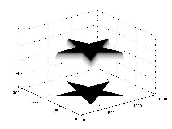
(a) The accumulated spectrogram plotted over the domain.

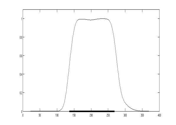
(b) A cross-section of the domain and the accumulated spectrogram.

Figure 2. A domain with the form of a star.

To argue that the tail in $\rho_{\Omega}$ is asymptotically smaller than ${|\Omega|}$ we consider dilations of a fixed set $\Omega$ and rescale $\rho_{R\cdot\Omega}$ by a factor of $R$. We then have the following result.

Theorem 1.3.

Let $g\in L^{2}({\mathbb{R}^{d}})$, $\lVert g\rVert_{2}=1$, and let $\Omega\subset{\mathbb{R}^{2d}}$ be compact. Then

$$\rho_{R\cdot\Omega}(R\cdot)\longrightarrow 1_{\Omega}\mbox{ in $L^{1}({\mathbb{R}^{2d}})$, as }R\longrightarrow+\infty.$$

Under mild regularity assumptions on $g$ and $\Omega$ we give a more quantitative and non-asymptotic estimate that explains the tail in $\rho_{\Omega}$ as an effect of the window $g$. To quantify the statement in Theorem 1.3, we assume that $g$ satisfies the following time-frequency concentration condition:

(7) $$\lVert g\rVert_{M^{*}}^{2}:=\int_{\mathbb{R}^{2d}}\left|z\right|\left|V_{g}g(z)\right|^{2}dz<+\infty.$$

We let ${M^{*}}({\mathbb{R}^{d}})$ denote the class of all $L^{2}({\mathbb{R}^{d}})$ functions satisfying (7). It follows easily that the Schwartz class is contained in ${M^{*}}({\mathbb{R}^{d}})$. (The class ${M^{*}}$ is closely related to the modulation spaces $M^{1}_{1}({\mathbb{R}^{d}})$ and $M^{2}_{1/2}({\mathbb{R}^{d}})$. See Remark 3.6).

In addition, we assume that $\Omega$ has finite perimeter. This means that its characteristic function $1_{\Omega}$ is of bounded variation. Every compact set $\Omega\subseteq{\mathbb{R}^{2d}}$ with smooth boundary has a finite perimeter and its perimeter is the $(2d-1)$-dimensional surface measure of its topological boundary. (Section 3.1 below provides more background on functions of bounded variation and sets of finite perimeter.)

Theorem 1.4.

Assume that $g\in{M^{*}}({\mathbb{R}^{d}})$ with $\lVert g\rVert_{2}=1$ and that $\Omega\subset{\mathbb{R}^{2d}}$ is a compact set with finite perimeter. Then

$$\frac{1}{{|\Omega|}}\bigl{\lVert}\rho_{\Omega}-1_{\Omega}*\left|V_{g}g\right|^{2}\bigr{\rVert}_{1}\leq\left(\frac{1}{{|\Omega|}}+4\lVert g\rVert_{M^{*}}\sqrt{\frac{\left|\partial{\Omega}\right|}{{|\Omega|}}}\right),$$

where $\left|\partial{\Omega}\right|$ is the perimeter of $\Omega$.

For ${|\Omega|}\geq 1$, Theorem 1.4 implies the weaker estimate

(8) $$\frac{1}{{|\Omega|}}\bigl{\lVert}\rho_{\Omega}-1_{\Omega}\bigr{\rVert}_{1}\leq C\sqrt{\frac{\left|\partial{\Omega}\right|}{{|\Omega|}}},$$

where the constant $C$ depends only on the window $g$ (see Corollary 5.1). Since $\lVert\rho_{\Omega}\rVert_{1}=A_{\Omega}={|\Omega|}+O(1)$ and $\lVert 1_{\Omega}\rVert_{1}={|\Omega|}$, the $L^{1}$-difference between $\rho_{\Omega}$ and $1_{\Omega}$ is much smaller than the norm of these two functions.

While (8) bounds the $L^{1}$-error (normalized over $\Omega$) incurred when approximating $\rho_{\Omega}$ by $1_{\Omega}$, it is even more interesting to obtain pointwise error estimates. Applying Chebyshev’s Inequality to (8), we obtain that

$$\Big{|}\left\{z\in\mathbb{R}^{2d}:\big{|}\rho_{\Omega}(z)-1_{\Omega}(z)\big{|}>\delta\right\}\Big{|}\lesssim\frac{\big{(}\left|\partial{\Omega}\right||\Omega|\big{)}^{1/2}}{\delta}\,.$$

As our final result we will prove the following refined weak-$L^{2}$ error estimate.

Theorem 1.5.

Let $g\in{M^{*}}({\mathbb{R}^{d}})$ and let $\Omega\subset{\mathbb{R}^{2d}}$ be a compact set with finite perimeter and assume that $\lVert g\rVert^{2}_{M^{*}}\left|\partial{\Omega}\right|\geq 1$. Then

$$\big{|}\left\{z\in\mathbb{R}^{2d}:\big{|}\rho_{\Omega}(z)-1_{\Omega}(z)\big{|}>\delta\right\}\big{|}\lesssim\frac{1}{\delta^{2}}\lVert g\rVert_{{M^{*}}}^{2}\left|\partial{\Omega}\right|,\qquad\delta>0.$$

Theorem 1.5 says that the size of the set where $\rho_{\Omega}$ differs significantly from $1_{\Omega}$ is of order $\left|\partial{\Omega}\right|$. This is the expected order: along the boundary $\partial\Omega$ the characteristic function $1_{\Omega}$ has a jump singularity, whereas the accumulated spectrogram $\rho_{\Omega}$ is smooth (at least uniformly continuous). Therefore $1_{\Omega}-\rho_{\Omega}$ must be large in a neighborhood of $\partial\Omega$, which suggests that $\left|\{z\in\mathbb{R}^{2d}:\big{|}\rho_{\Omega}(z)-1_{\Omega}(z)\big{|}>\delta\right|\}\geq c_{\delta}\left|\partial{\Omega}\right|$.

For a numerical illustration of Theorem 1.5 see Figure 2.

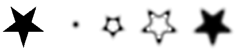
(a) A domain of area $\approx$ 23, the spectrograms of the eigenfunctions for $k=1,7$ and $17$, and the accumulated spectrogram with respect to the Gaussian $g(t)=2^{1/4}e^{-\pi t^{2}}$. The shading of each eigenfunction is relative to its own scale of values.

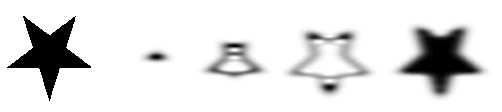
(b) The same experiment with the Gaussian window $g(t)=2^{-1/4}e^{-\pi(t/2)^{2}}$, that is is more concentrated in frequency than the Gaussian in (a)

Figure 3. The first eigenfunctions of a time-frequency localization operator with identical domain $\Omega$, but with different windows. One obtains two different (almost) partitions of unity on the same domain.

1.3. Universality

In general, the individual eigenfunctions and their spectrograms are difficult to describe, since they depend on the underlying window $g$ in an intricate manner (see Figure 3). Nevertheless, by (8) the spectrograms of the whole family $\{h^{\Omega}_{1},\ldots,h^{\Omega}_{A_{\Omega}}\}$ almost form a partition of unity on $\Omega$. By and large this property is independent of the window $g$ (which enters only through some constants in the error estimates). Even more is true: the asymptotic result of Theorem 1.3 is completely independent of $g$.

In mathematics, the term “universality” is used to describe phenomena where properties of complex systems simplify in an asymptotic regime and then depend only on few parameters. The primary examples are the central limit theorem in probability or the eigenvalue distribution of random matrices. (See [9] for an overview of universality in several contexts.)

In this sense, Theorem 1.3 expresses a new and intriguing universality property. Whereas the accumulated spectrograms for a fixed domain with different windows may display a vastly different behavior for small scales, they all approach the characteristic function in the scaling limit $R\to\infty$. See Figure 3.

The universality property expressed by Theorem 1.3 has also a probabilistic interpretation. Consider the finite dimensional space generated by the short-time Fourier transform of the first $A_{\Omega}$ eigenfunctions of $H_{\Omega}$ and its associated reproducing kernel. The accumulated spectrogram is the one-point intensity of the determinantal point process associated with this reproducing kernel (see [4] for precise definitions). Thus, Theorem 1.3 asserts that the asymptotic limit of this one-point intensity is the uniform distribution on $\Omega$, independently of the chosen window g.

1.4. Ginibre’s law

It is instructive to discuss a case where all the objects can be computed explicitly. Let $g(t):=2^{1/4}e^{-\pi t^{2}}$, $t\in{\mathbb{R}}$, be the one-dimensional, $L^{2}$-normalized Gaussian and let

$${\mathbb{D}}:=\big{\{}\,(x,\xi)\in{\mathbb{R}}^{2}\,:\,x^{2}+\xi^{2}\leq 1\,\big{\}}$$

be the unit disk. By a result of Daubechies [7] the eigenfunctions and eigenvalues of the time-frequency localization operator with window $g$ and domain $\Omega=R\cdot{\mathbb{D}}$ for arbitrary $R>0$ are the Hermite functions

(9) $$h_{k+1}(t)=\frac{2^{1/4}}{\sqrt{k!}}\left(\frac{-1}{2\sqrt{\pi}}\right)^{k}e^{\pi t^{2}}\frac{d^{k}}{dt^{k}}\left(e^{-2\pi t^{2}}\right),\qquad k\geq 0.$$

Remarkably, due to the symmetries of $g$ and ${\mathbb{D}}$, the eigenfunctions $h_{k}$ of $H_{R{\mathbb{D}}}$ do not depend on $R$. Identifying $z=(x,\xi)\in\mathbb{R}^{2}$ with $z:=x+i\xi\in{\mathbb{C}}$, the short-time Fourier transform of the Hermite functions with respect to $g$ is

$$V_{g}h_{k+1}(\bar{z})=e^{\pi ix\xi}\left(\frac{\pi^{k}}{k!}\right)^{1/2}z^{k}e^{-\pi\left|z\right|^{2}/2},\qquad k\geq 0.$$

Hence the corresponding spectrograms are

$$\left|V_{g}h_{k+1}(z)\right|^{2}=\frac{\pi^{k}}{k!}\left|z\right|^{2k}e^{-\pi\left|z\right|^{2}},\qquad k\geq 0,$$

and the accumulated spectrogram corresponding to $R\cdot{\mathbb{D}}$ is

$$\rho_{R\cdot{\mathbb{D}}}(z)=\sum_{k=0}^{\lceil\pi R^{2}\rceil-1}\frac{\pi^{k}}{k!}\left|z\right|^{2k}e^{-\pi\left|z\right|^{2}}.$$

Theorem 1.3 says that

$$\rho_{R\cdot{\mathbb{D}}}(Rz)=\sum_{k=0}^{\lceil\pi R^{2}\rceil-1}\frac{\pi^{k}}{k!}R^{2k}\left|z\right|^{2k}e^{-\pi\left|Rz\right|^{2}}\longrightarrow 1_{\mathbb{D}}(z),\mbox{ in }L^{1}({\mathbb{C}},dxd\xi)\mbox{ as }n\longrightarrow+\infty.$$

This formula is one of Ginibre’s limit laws [17]. (Of course, in this case more precise asymptotic estimates are possible.)

1.5. Technical overview

As commonly done in the literature, we transfer the problem to the range of the short-time Fourier transform $V_{g}L^{2}({\mathbb{R}^{d}})$. This is a reproducing kernel subspace of $L^{2}({\mathbb{R}^{2d}})$ and the time-frequency localization operator ${H_{\Omega}}$ translates into a Toeplitz operator on $V_{g}L^{2}({\mathbb{R}^{d}})$.

Our proof begins with the observation that $\rho_{\Omega}$ is the diagonal of the integral kernel of the orthogonal projection operator $P_{n}$ from $V_{g}L^{2}({\mathbb{R}^{d}})$ onto the linear span of the functions $\left\{V_{g}h^{\Omega}_{1},\ldots,V_{g}h^{\Omega}_{n}\right\}$. We then compare $P_{n}$ to the Toeplitz operator, which has an explicit integral kernel for which we derive direct estimates. The relation between the Toeplitz operator and $P_{n}$ can be understood as a threshold on its eigenvalues. We then resort to the rich existing literature on these [10, 15, 19, 20, 22, 23, 24, 27, 33].

1.6. Organization

Section 2 introduces some basic tools from time-frequency analysis, including the interpretation of time-frequency localization operators as Toeplitz operators on a certain reproducing kernel space. In Section 3 we recall the estimates on the profile of the eigenvalues of time-frequency localization operators, and add a slight refinement. Section 4 develops a number of technical estimates that are used in Section 5 to prove the main results. Finally, Section 6 briefly presents an application of Theorem 1.5 to signal processing.

2. Phase-space tools

We now introduce the basic phase-space tools related to the short-time Fourier transform.

2.1. The range of the short-time Fourier transform

Throughout the article we fix a window $g\in L^{2}({\mathbb{R}^{d}})$ with normalization $\lVert g\rVert_{2}=1$. The short-time Fourier transform with respect to $g$ - cf. (1) - then defines an isometry $V_{g}:L^{2}({\mathbb{R}^{d}})\to L^{2}({\mathbb{R}^{2d}})$. (This is a consequence of Plancherel’s theorem, see for example [18, Chapter 1]). The adjoint of $V_{g}$ is $V^{*}_{g}:L^{2}({\mathbb{R}^{2d}})\to L^{2}({\mathbb{R}^{d}})$

$$V^{*}_{g}F(t)=\int_{{\mathbb{R}^{d}}\times{\mathbb{R}^{d}}}F(x,\xi)g(t-x)e^{2\pi i\xi t}dxd\xi,\qquad t\in{\mathbb{R}^{d}}.$$

Let ${\mathbb{H}}:=V_{g}L^{2}({\mathbb{R}^{d}})\subseteq L^{2}({\mathbb{R}^{2d}})$ be the (closed) range of $V_{g}$. The orthogonal projection $P_{\mathbb{H}}:L^{2}({\mathbb{R}^{2d}})\to{\mathbb{H}}$ is given by $P_{\mathbb{H}}=V_{g}V^{*}_{g}$. Explicitly, $P_{\mathbb{H}}$ is the integral operator

(10) $$P_{\mathbb{H}}F(z) =\int_{\mathbb{R}^{2d}}F(z^{\prime})K(z,z^{\prime})dz^{\prime},\qquad z=(x,\xi)\in{\mathbb{R}^{2d}},$$

with integral kernel

(11) $$K(z,z^{\prime})=V_{g}g(z-z^{\prime})e^{2\pi i\xi x^{\prime}},\qquad z=(x,\xi),z^{\prime}=(x^{\prime},\xi^{\prime})\in{\mathbb{R}^{2d}}.$$

Using this description of $P_{\mathbb{H}}$ it follows that ${\mathbb{H}}$ is a reproducing kernel Hilbert subspace of ${L^{2}({\mathbb{R}^{2d}})}$. This means that each function $F\in{\mathbb{H}}$ is continuous and satisfies $F(z)=\int F(z^{\prime})K(z,z^{\prime})dz^{\prime}$ for all $z\in{\mathbb{R}^{2d}}$. The function $K$ is called the reproducing kernel of ${\mathbb{H}}$.

Since $K$ is the integral kernel of an orthogonal projection, it satisfies $K(z,z^{\prime})=\overline{K(z^{\prime},z)}$ and

(12) $$K(z,z^{\prime})=\int_{\mathbb{R}^{2d}}K(z,z^{\prime\prime})K(z^{\prime\prime},z^{\prime})dz^{\prime\prime},\qquad z,z^{\prime}\in{\mathbb{R}^{2d}}.$$

In addition, if $\left\{E_{k}:k\geq 1\right\}$ is an orthonormal basis of ${\mathbb{H}}$, $K$ can be expanded as

(13) $$K(z,z^{\prime})=\sum_{k\geq 1}E_{k}(z)\overline{E_{k}(z^{\prime})},\qquad z,z^{\prime}\in{\mathbb{R}^{2d}}.$$

From now on, we use the notation

$$\Theta(z):=\left|V_{g}g(z)\right|^{2},\qquad z\in{\mathbb{R}^{2d}}.$$

Then $\Theta\in L^{1}({\mathbb{R}^{2d}})$, $\int_{\mathbb{R}^{2d}}\Theta=\int_{\mathbb{R}^{2d}}|V_{g}g|^{2}=\|g\|_{2}^{4}=1$, $\Theta(z)=\Theta(-z)$ and

(14) $$\left|K(z,z^{\prime})\right|^{2}=\Theta(z-z^{\prime}),\qquad z,z^{\prime}\in{\mathbb{R}^{2d}}.$$

2.2. Time-frequency localization and Toeplitz operators

Using $V_{g}$ and $V^{*}_{g}$, the time-frequency localization operator ${H_{\Omega}}:L^{2}({\mathbb{R}^{d}})\to L^{2}({\mathbb{R}^{d}})$ from (3) can be written as

$${H_{\Omega}}f=V^{*}_{g}(1_{\Omega}\cdot V_{g}f),\qquad f\in{L^{2}({\mathbb{R}^{d}})}.$$

Therefore,

(15) $$(V_{g}{H_{\Omega}}V^{*}_{g})F=P_{\mathbb{H}}(1_{\Omega}\cdot F),\qquad F\in{\mathbb{H}}.$$

Hence, if we define the Gabor-Toeplitz operator $M_{\Omega}:{\mathbb{H}}\to{\mathbb{H}}$ as

$$M_{\Omega}F:=P_{\mathbb{H}}(1_{\Omega}\cdot F),\qquad F\in{\mathbb{H}},$$

then (15) says that ${H_{\Omega}}$ and $M_{\Omega}$ are related by

(16) $$V^{*}_{g}M_{\Omega}V_{g}={H_{\Omega}}.$$

As a consequence, $M_{\Omega}$ and ${H_{\Omega}}$ enjoy the same spectral properties. Using the diagonalization of ${H_{\Omega}}$ in (4) and the notation

$$H^{\Omega}_{k}=V_{g}h^{\Omega}_{k},\qquad k\geq 1,$$

$M_{\Omega}$ can be diagonalized as

(17) $$M_{\Omega}F=\sum_{k\geq 1}{\lambda_{k}^{\Omega}}\left<F,H^{\Omega}_{k}\right>H^{\Omega}_{k},\qquad F\in{\mathbb{H}}.$$

In addition, the accumulated spectrogram can be written as

$$\rho_{\Omega}(z)=\sum_{k=1}^{A_{\Omega}}\left|H^{\Omega}_{k}(z)\right|^{2},\qquad z\in{\mathbb{R}^{2d}}.$$

Since $\left\{H^{\Omega}_{k}:k\geq 1\right\}$ is an orthonormal subset of ${\mathbb{H}}$ and $K(z,z)=1$, it follows from (13) that

(18) $$\sum_{k\geq 1}\left|H^{\Omega}_{k}(z)\right|^{2}\leq 1,\qquad z\in{\mathbb{R}^{2d}},$$

and consequently, the accumulated spectrogram satisfies

(19) $$0\leq\rho_{\Omega}(z)\leq 1,\qquad z\in{\mathbb{R}^{2d}}.$$

2.3. Properties of Toeplitz operators

Using (10) we see that $M_{\Omega}:{\mathbb{H}}\to{\mathbb{H}}$ can be described as

$$M_{\Omega}F(z)=\int_{\Omega}F(z^{\prime})K(z,z^{\prime})dz^{\prime},\qquad z\in{\mathbb{R}^{2d}}.$$

We now note some simple properties of Toeplitz operators. These are well-known [5, 6, 10, 11, 12, 15], but are normally stated in a slightly different form. Therefore we sketch a short proof.

Lemma 2.1.

Let $g\in L^{2}({\mathbb{R}^{d}})$ with $\lVert g\rVert_{2}=1$ and let $\Omega\subseteq{\mathbb{R}^{2d}}$ be a compact set. Then $M_{\Omega}:L^{2}({\mathbb{R}^{d}})\to L^{2}({\mathbb{R}^{d}})$ is trace-class and satisfies

(20) $$0\leq M_{\Omega}\leq I.$$

The traces of $M_{\Omega}$ and $M_{\Omega}^{2}$ are given by

(21) $$\mathrm{trace}(M_{\Omega})=\int_{\Omega}K(z,z)dz={|\Omega|},$$

(22) $$\mathrm{trace}(M_{\Omega}^{2})=\int_{\Omega}\int_{\Omega}\Theta(z-z^{\prime})dzdz^{\prime}.$$

Proof.

For $F\in{\mathbb{H}}$ we compute

$$\left<M_{\Omega}F,F\right>=\left<P_{\mathbb{H}}(1_{\Omega}F),F\right>=\left<1_{\Omega}F,F\right>=\int_{\Omega}\left|F(z)\right|^{2}dz.$$

This gives (20), and in particular shows that $M_{\Omega}$ is bounded and positive.

Let $\mathcal{M}_{\Omega}:L^{2}({\mathbb{R}^{2d}})\to L^{2}({\mathbb{R}^{2d}})$ be the inflated operator $\mathcal{M}_{\Omega}(F):=P_{\mathbb{H}}(1_{\Omega}\cdot P_{\mathbb{H}}(F))$. Hence, with respect to the decomposition $L^{2}({\mathbb{R}^{2d}})={\mathbb{H}}\oplus{\mathbb{H}}^{\perp}$, $\mathcal{M}_{\Omega}$ is given by

(25) $$\mathcal{M}_{\Omega}=\left[\begin{array}[]{ll}M_{\Omega}&0\\ 0&0\end{array}\right].$$

Since $\mathcal{M}_{\Omega}$ is defined on $L^{2}({\mathbb{R}^{2d}})$, its spectral properties can be easily related to its integral kernel. Using (10) we get the following formula for $\mathcal{M}_{\Omega}$

$$\mathcal{M}_{\Omega}F(z)=\int_{\mathbb{R}^{2d}}F(z^{\prime})\int_{\mathbb{R}^{2d}}1_{\Omega}(z^{\prime\prime})K(z,z^{\prime\prime})K(z^{\prime\prime},z^{\prime})dz^{\prime\prime}dz^{\prime},\qquad F\in L^{2}({\mathbb{R}^{2d}}).$$

That is, $\mathcal{M}_{\Omega}$ has integral kernel $K_{\mathcal{M}_{\Omega}}(z,z^{\prime}):=\int 1_{\Omega}(z^{\prime\prime})K(z,z^{\prime\prime})K(z^{\prime\prime},z^{\prime})dz^{\prime\prime}$.

Using (14) we compute

$$\int_{\mathbb{R}^{2d}}K_{\mathcal{M}_{\Omega}}(z,z)dz=\int_{\mathbb{R}^{2d}}\int_{\mathbb{R}^{2d}}1_{\Omega}(z^{\prime})\Theta(z-z^{\prime})dzdz^{\prime}={|\Omega|}\lVert\Theta\rVert_{1}={|\Omega|}.$$

Since $M_{\Omega}$ is positive, so is $\mathcal{M}_{\Omega}$ by (25). Hence, the previous calculation shows that $\mathcal{M}_{\Omega}$ is trace-class and $\mathrm{trace}(\mathcal{M}_{\Omega})={|\Omega|}$ (see for example [35, Theorems 2.12 and 2.14]). Using (25) we deduce that $M_{\Omega}$ is trace class and $\mathrm{trace}(M_{\Omega})=\mathrm{trace}(\mathcal{M}_{\Omega})={|\Omega|}$. For (22), we use again the fact that $\mathcal{M}_{\Omega}$ is positive to get

$$\mathrm{trace}(M_{\Omega}^{2})=\mathrm{trace}(\mathcal{M}_{\Omega}^{2})=\lVert K_{\mathcal{M}_{\Omega}}\rVert_{2}^{2}$$

$$\quad=\int_{{\mathbb{R}^{2d}}}\int_{{\mathbb{R}^{2d}}}K_{\mathcal{M}_{\Omega}}(z,z^{\prime})K_{\mathcal{M}_{\Omega}}(z^{\prime},z)dzdz^{\prime}$$

$$\quad=\int_{{\mathbb{R}^{2d}}}\int_{{\mathbb{R}^{2d}}}1_{\Omega}(w)1_{\Omega}(w^{\prime})\int_{{\mathbb{R}^{2d}}}\int_{{\mathbb{R}^{2d}}}K(z,w)K(w,z^{\prime})K(z^{\prime},w^{\prime})K(w^{\prime},z)dzdz^{\prime}dwdw^{\prime}.$$

Using (12) and (14) it follows that

$$\mathrm{trace}(M_{\Omega}^{2}) =\int_{{\mathbb{R}^{2d}}}\int_{{\mathbb{R}^{2d}}}1_{\Omega}(w)1_{\Omega}(w^{\prime})K(w,w^{\prime})K(w^{\prime},w)dwdw^{\prime}$$

$$=\int_{{\mathbb{R}^{2d}}}\int_{{\mathbb{R}^{2d}}}1_{\Omega}(w)1_{\Omega}(w^{\prime})\Theta(w-w^{\prime})dwdw^{\prime},$$

as desired. ∎

3. Profile of the eigenvalues

Let $g\in{L^{2}({\mathbb{R}^{d}})}$, $\lVert g\rVert_{2}=1$, and consider the time-frequency localization operator ${H_{\Omega}}$ associated with a compact set $\Omega$. The fundamental asymptotic behavior of the profile of the eigenvalues $\left\{{\lambda_{k}^{\Omega}}:k\geq 1\right\}$ are given by Proposition 1.1, and were obtained by Ramanathan and Topiwala in a weaker form and by Feichtinger and Nowak in full generality [15, 33].

For sets with smooth boundary, Ramanathan and Topiwala [33] quantified the order of convergence in (6). Later De Mari, Feichtinger and Nowak obtained fine asymptotics for families of sets where certain geometric quantities are kept uniform [10] - the dilations of a set with smooth boundary being one such an example. Moreover their results are also applicable to the hyperbolic setting [10].

We will need a variation of the result in [33].

3.1. Functions of bounded variation

We first collect some basic facts about functions of bounded variation. A real-valued function $f\in L^{1}({\mathbb{R}^{d}})$ is said to have bounded variation, $f\in\textit{BV}({\mathbb{R}^{d}})$, if its distributional partial derivatives are finite Radon measures. The variation of $f$ is defined as

$$\textit{Var}(f):=\sup\left\{\int_{\mathbb{R}^{d}}f(x)\operatorname{div}\phi(x)dx:\phi\in C^{1}_{c}({\mathbb{R}^{d}},{\mathbb{R}^{d}}),\left|\phi(x)\right|_{2}\leq 1\right\}\,,$$

where $C^{1}_{c}({\mathbb{R}^{d}},{\mathbb{R}^{d}})$ denotes the class of compactly supported $C^{1}$-vector fields and $\operatorname{div}$ is the divergence operator.

If $f$ is continuously differentiable, then $f\in\textit{BV}({\mathbb{R}^{d}})$ simply means that $\partial_{x_{1}}f,\ldots$, $\partial_{x_{d}}f\in L^{1}({\mathbb{R}^{d}})$, and $\textit{Var}(f)=\int_{\mathbb{R}^{d}}\left|\nabla f(x)\right|_{2}dx$.

A set $E\subseteq{\mathbb{R}^{d}}$ is said to have finite perimeter if its characteristic function $1_{E}$ is of bounded variation, and the perimeter of $E$ is $\left|\partial{E}\right|:=\textit{Var}(1_{E})$. If $E$ has a smooth boundary, then $\left|\partial{E}\right|$ is just the $(2d-1)$-Hausdorff measure of the topological boundary. See [13, Chapter 5] for an extensive discussion of BV.

We will use the following approximation result from  [13, Sec. 5.2.2, Thm. 2].

Proposition 3.1.

Let $f\in\textit{BV}({\mathbb{R}^{d}})$. Then there exists $\left\{f_{k}:k\geq 1\right\}\subseteq\textit{BV}({\mathbb{R}^{d}})\cap C^{\infty}({\mathbb{R}^{d}})$ such that $f_{k}\longrightarrow f$ in $L^{1}({\mathbb{R}^{d}})$ and $\int\left|\nabla f_{k}(x)\right|_{2}dx\longrightarrow\textit{Var}(f)$, as $k\longrightarrow+\infty$.

Note that this proposition does not assert that $\textit{Var}(f-f_{k})\longrightarrow 0$.

The following lemma quantifies the error introduced by regularization.

Lemma 3.2.

Let $f\in\textit{BV}({\mathbb{R}^{d}})$ and $\varphi\in{L^{1}({\mathbb{R}^{d}})}$ with $\int\varphi=1$. Then

$$\lVert f*\varphi-f\rVert_{1}\leq\textit{Var}(f)\int_{\mathbb{R}^{d}}\left|x\right|_{2}\left|\varphi(x)\right|dx.$$

Proof.

Assume first that $f\in C^{\infty}({\mathbb{R}^{d}})$ and estimate

$$\lVert f*\varphi-f\rVert_{1}=\int_{\mathbb{R}^{d}}\left|\int_{\mathbb{R}^{d}}f(y)\varphi(x-y)\,dy-f(x)\right|dx$$

$$\qquad=\int_{\mathbb{R}^{d}}\left|\int_{\mathbb{R}^{d}}(f(y)-f(x))\varphi(x-y)\,dy\right|dx$$

$$\qquad=\int_{\mathbb{R}^{d}}\left|\int_{\mathbb{R}^{d}}(f(x)-f(y))\varphi(x-y)\,dy\right|dx$$

$$\qquad=\int_{\mathbb{R}^{d}}\left|\int_{\mathbb{R}^{d}}\int_{0}^{1}\left<\nabla f(t(x-y)+y),x-y\right>\varphi(x-y)dtdy\right|dx$$

$$\qquad\leq\int_{0}^{1}\int_{\mathbb{R}^{d}}\int_{\mathbb{R}^{d}}\left|\nabla f(t(x-y)+y)\right|_{2}\left|x-y\right|_{2}\left|\varphi(x-y)\right|dxdydt$$

$$\qquad=\int_{0}^{1}\int_{\mathbb{R}^{d}}\int_{\mathbb{R}^{d}}\left|\nabla f(tx+y)\right|_{2}\left|x\right|_{2}\left|\varphi(x)\right|dxdydt$$

$$\qquad=\bigl{\lVert}\left|\nabla f\right|_{2}\bigr{\rVert}_{1}\int_{\mathbb{R}^{d}}\left|x\right|_{2}\left|\varphi(x)\right|dx.$$

For an arbitrary function of bounded variation $f$, Proposition 3.1 implies the existence of a sequence $\left\{f_{k}:k\geq 1\right\}\subseteq BV({\mathbb{R}^{d}})\cap C^{\infty}({\mathbb{R}^{d}})$ such that $f_{k}\longrightarrow f$ in $L^{1}$ and $\bigl{\lVert}\left|\nabla f_{k}\right|_{2}\bigr{\rVert}_{1}\longrightarrow\textit{Var}(f)$. The desired estimate now follows by approximation. ∎

3.2. Estimates on eigenvalues

We now quote the standard estimate for the eigenvalue distribution. This estimate is ubiquitous in the literature - see for example [24, Thm. 1], [33, Thm. 2] or [15, Remark (iii)]. For lack of an exact quotable reference we sketch a proof following [15].

Lemma 3.3.

Let $g\in{L^{2}({\mathbb{R}^{d}})}$, $\lVert g\rVert_{2}=1$, and let $\Omega\subset{\mathbb{R}^{2d}}$ be compact. Then for $\delta\in(0,1)$,

$$\Big{|}\#\left\{k\geq 1:{\lambda_{k}^{\Omega}}>1-\delta\right\}-{|\Omega|}\Big{|}\leq\max\left\{\frac{1}{\delta},\frac{1}{1-\delta}\right\}\left|\int_{\Omega}\int_{\Omega}\Theta(z-z^{\prime})dzdz^{\prime}-{|\Omega|}\right|.$$

Proof.

Let $\delta\in(0,1)$ and $G:[0,1]\to{\mathbb{R}}$ be the function

$$G(t):=\left\{\begin{array}[]{ll}-t,&\mbox{if }0\leq t\leq 1-\delta,\\ 1-t,&\mbox{if }1-\delta<t\leq 1.\end{array}\right.$$

and note that $\left|G(t)\right|\leq\max\left\{\frac{1}{\delta},\frac{1}{1-\delta}\right\}(t-t^{2})$ for $t\in[0,1]$. Since $0\leq M_{\Omega}\leq 1$ we estimate

$$\Big{|}\#\left\{k\geq 1:{\lambda_{k}^{\Omega}}>1-\delta\right\}-{|\Omega|}\Big{|}=\left|\mathrm{trace}(G(M_{\Omega}))\right|\leq\mathrm{trace}(\left|G\right|(M_{\Omega}))$$

$$\qquad\leq\max\left\{\frac{1}{\delta},\frac{1}{1-\delta}\right\}\mathrm{trace}(M_{\Omega}-M_{\Omega}^{2}).$$

The formulas in Lemma 2.1 complete the proof. ∎

Finally, we obtain the following estimate, which is a variation of the result in [33]. While [33] uses the co-area formula, we resort to Lemma 3.2.

Proposition 3.4.

Let $\Omega\subset{\mathbb{R}^{2d}}$ be a compact set with finite perimeter and assume that $g\in{M^{*}}({\mathbb{R}^{d}})$. Then for each $\delta\in(0,1)$,

$$\Big{|}\#\left\{k:{\lambda_{k}^{\Omega}}>1-\delta\right\}-{|\Omega|}\Big{|}\leq\max\left\{\frac{1}{\delta},\frac{1}{1-\delta}\right\}\lVert g\rVert_{{M^{*}}}^{2}\left|\partial{\Omega}\right|.$$

Proof.

Recall that $\Theta(z)=\left|V_{g}g(z)\right|^{2}=\Theta(-z)$, let $F:=1_{\Omega}$ and note that

$$\left|\int_{\Omega}\int_{\Omega}\Theta(z-z^{\prime})dzdz^{\prime}-{|\Omega|}\right|=\left|\int_{\Omega}(F*\Theta)(z^{\prime})-F(z^{\prime})dz^{\prime}\right|\leq\lVert F*\Theta-F\rVert_{1}.$$

We now combine Lemmas 3.2 and 3.3 and the desired conclusion follows. ∎

Remark 3.5.

The results in [10] provide an asymptotic converse inequality to the estimate in Proposition 3.4, showing that for certain classes of sets and small $\delta$, the error $\left|\#\left\{k:{\lambda_{k}^{\Omega}}>1-\delta\right\}-{|\Omega|}\right|$ is also bounded from below by $\left|\partial{\Omega}\right|$.

Remark 3.6.

The class ${M^{*}}({\mathbb{R}^{d}})$ is closely related to certain modulation spaces. Modulation spaces are Banach spaces of distributions $f$ defined by decay conditions of the short-time Fourier transform $V_{\phi}f$ with respect to a fixed Schwartz function $\phi$. In particular, the spaces $M^{1}_{1}({\mathbb{R}^{d}})$ and $M^{2}_{1/2}({\mathbb{R}^{d}})$ are defined by the norms

$$\lVert f\rVert_{M^{1}_{1}} :=\int_{\mathbb{R}^{d}}\left|z\right|\left|V_{\phi}f(z)\right|dz,$$

$$\lVert f\rVert^{2}_{M^{2}_{1/2}} :=\int_{\mathbb{R}^{d}}\left|z\right|\left|V_{\phi}f(z)\right|^{2}dz.$$

It is then easy to see that $M^{1}_{1}({\mathbb{R}^{d}})\subseteq{M^{*}}({\mathbb{R}^{d}})\subseteq M^{2}_{1/2}({\mathbb{R}^{d}})$. Easy sufficient condition for the membership in $M^{1}_{1}({\mathbb{R}^{d}})$ and $M^{*}({\mathbb{R}^{d}})$ can be given by means of embeddings of Fourier-Lebesgue spaces in modulation spaces [16]. For instance, if

$$\int_{{\mathbb{R}^{d}}}\Big{(}|g(x)|^{2}+|\hat{g}(x)|^{2}\Big{)}\,(1+|x|^{2})^{1/d+1/2+\epsilon}\,dx<\infty$$

for some $\epsilon>0$, then $g\in M^{1}_{1}({\mathbb{R}^{d}})\subseteq M^{*}({\mathbb{R}^{d}})$. For the theory of modulation spaces we refer to  [18], for a historical overview see [14].

4. Some technical estimates

We now derive a number of lemmas. In the next section we combine them in several ways to obtain the main results. Recall that we always assume that $g\in L^{2}({\mathbb{R}^{d}})$ and $\lVert g\rVert_{2}=1$. We use the notation from Section 2. The following lemma is one of the key observations in our proof.

Lemma 4.1.

Let $\Omega\subset{\mathbb{R}^{2d}}$ be a compact set. Then the following formula holds

$$(1_{\Omega}*\Theta)(z)=\sum_{k\geq 1}{\lambda_{k}^{\Omega}}\left|H^{\Omega}_{k}(z)\right|^{2},\quad z\in{\mathbb{R}^{2d}}.$$

Proof.

Let $K(z,z^{\prime})=V_{g}g(z-z^{\prime})e^{2\pi iz_{2}z^{\prime}_{1}}$ be the reproducing kernel of ${\mathbb{H}}$ and $K_{z}:=\overline{K(z,\cdot)}\in{\mathbb{H}}$. Hence for all $F\in{\mathbb{H}}$,

$$F(z)=\int_{{\mathbb{R}^{2d}}}K(z,z^{\prime})F(z^{\prime})\,dz^{\prime}=\left<F,K_{z}\right>,\qquad z\in{\mathbb{R}^{2d}}.$$

First we compute

$$\left<M_{\Omega}K_{z},K_{z}\right> =\left<1_{\Omega}K_{z},K_{z}\right>$$

$$=\int_{{\mathbb{R}^{2d}}}1_{\Omega}(z^{\prime})K_{z}(z^{\prime})\overline{K_{z}(z^{\prime})}\,dz^{\prime}$$

$$=\int_{{\mathbb{R}^{2d}}}1_{\Omega}(z^{\prime})\Theta(z-z^{\prime})\,dz^{\prime}=(1_{\Omega}*\Theta)(z).$$

Second, we use (17) to compute

$$\left<M_{\Omega}K_{z},K_{z}\right> =\left<\sum_{k}{\lambda_{k}^{\Omega}}\left<K_{z},H^{\Omega}_{k}\right>H^{\Omega}_{k},K_{z}\right>$$

$$=\sum_{k}{\lambda_{k}^{\Omega}}\left|\left<H^{\Omega}_{k},K_{z}\right>\right|^{2}$$

$$=\sum_{k}{\lambda_{k}^{\Omega}}\left|H^{\Omega}_{k}(z)\right|^{2}.$$

The lemma follows by equating the two formulae for $\left<M_{\Omega}K_{z},K_{z}\right>$. ∎

We now use Lemma 4.1 to bound the error between $\rho_{\Omega}$ and $1_{\Omega}$.

Lemma 4.2.

Let $\Omega\subset{\mathbb{R}^{2d}}$ be compact and set

(26) $$E(\Omega):=1-\frac{\sum_{k=1}^{A_{\Omega}}{\lambda_{k}^{\Omega}}}{{|\Omega|}}.$$

Then

$$\frac{1}{{|\Omega|}}\bigl{\lVert}\rho_{\Omega}-(1_{\Omega}*\Theta)\bigr{\rVert}_{1}\leq\left(\frac{1}{{|\Omega|}}+2E(\Omega)\right).$$

Proof.

Let us set $L_{k}:=1$ for $1\leq k\leq A_{\Omega}$ and $L_{k}:=0$ for $k>A_{\Omega}$. Using Lemma 4.1 we have that

(27) $$\rho_{\Omega}(z)-(1_{\Omega}*\Theta)(z)=\sum_{k\geq 1}(L_{k}-\lambda^{\Omega}_{k})\left|H^{\Omega}_{k}(z)\right|^{2}.$$

Since $\bigl{\lVert}\left|H^{\Omega}_{k}\right|^{2}\bigr{\rVert}_{1}=\bigl{\lVert}V_{g}h_{k}^{\Omega}\bigr{\rVert}_{2}^{2}=\lVert h^{\Omega}_{k}\rVert_{2}^{2}=1$, we use (21) and estimate

$$\bigl{\lVert}\rho_{\Omega}-(1_{\Omega}*\Theta)\bigr{\rVert}_{1}\leq\left(\sum_{k\geq 1}\left|L_{k}-\lambda^{\Omega}_{k}\right|\right)=\left(\sum_{k=1}^{A_{\Omega}}(1-\lambda^{\Omega}_{k})+\sum_{k>A_{\Omega}}\lambda^{\Omega}_{k}\right)$$

$$\qquad=\left(A_{\Omega}-2\sum_{k=1}^{A_{\Omega}}\lambda^{\Omega}_{k}+\sum_{k\geq 1}\lambda^{\Omega}_{k}\right)=\left(A_{\Omega}-2\sum_{k=1}^{A_{\Omega}}\lambda^{\Omega}_{k}+{|\Omega|}\right)$$

$$\qquad=\left((A_{\Omega}-{|\Omega|})+2({|\Omega|}-\sum_{k=1}^{A_{\Omega}}\lambda^{\Omega}_{k})\right)\leq\left(1+2({|\Omega|}-\sum_{k=1}^{A_{\Omega}}\lambda^{\Omega}_{k})\right)$$

$$\qquad=1+2E(\Omega){|\Omega|}.$$

∎

The tail of the eigenvalue distribution $E(\Omega)$ can be estimated as follows.

Lemma 4.3.

Let $\Omega\subset{\mathbb{R}^{2d}}$ be a compact set and consider the number $E(\Omega)$ defined in (26). Then the following holds.

• $E(R\cdot\Omega)\longrightarrow 0$, as $R\longrightarrow+\infty$.

• If $\Omega$ has finite perimeter and $g\in{M^{*}}$, then

  (28) $$0\leq E(\Omega)\leq 2\lVert g\rVert_{M^{*}}\sqrt{\frac{\left|\partial{\Omega}\right|}{{|\Omega|}}}.$$

Proof.

First note that from (21) we know that $\sum_{k}{\lambda_{k}^{\Omega}}={|\Omega|}$ and consequently $0\leq E(\Omega)\leq 1$.

Let $\delta\in(0,1)$ and define $l_{\delta}(\Omega):=\min\{A_{\Omega},\#\left\{k:{\lambda_{k}^{\Omega}}>1-\delta\right\}\}$. Then

$${\lambda_{k}^{\Omega}}\geq 1-\delta\mbox{ for }1\leq k\leq l_{\delta}(\Omega).$$

Since $A_{\Omega}\geq l_{\delta}(\Omega)$ we estimate

$$\sum_{k=1}^{A_{\Omega}}{\lambda_{k}^{\Omega}}\geq\sum_{k=1}^{l_{\delta}(\Omega)}{\lambda_{k}^{\Omega}}\geq(1-\delta)l_{\delta}(\Omega).$$

Therefore,

$$0\leq E(\Omega) \leq 1-(1-\delta)\frac{l_{\delta}(\Omega)}{{|\Omega|}}.$$

Since $A_{\Omega}\geq{|\Omega|}$ we get

(29) $$0\leq E(\Omega)\leq 1-(1-\delta)\min\left\{1,\frac{\#\left\{k:{\lambda_{k}^{\Omega}}>1-\delta\right\}}{{|\Omega|}}\right\}.$$

To prove (a), we apply this estimate and Proposition 1.1 to $R\cdot\Omega$ to deduce that

$$0\leq\limsup_{R\rightarrow+\infty}E(R\cdot\Omega)\leq 1-(1-\delta)=\delta,$$

and then let $\delta\longrightarrow 0^{+}$.

To prove (b), we apply Proposition 3.4 and obtain

$$\frac{\#\left\{k:{\lambda_{k}^{\Omega}}>1-\delta\right\}}{{|\Omega|}}\geq 1-C_{\delta}\lVert g\rVert_{{M^{*}}}^{2}\frac{\left|\partial{\Omega}\right|}{{|\Omega|}},$$

where $C_{\delta}=\max\{\delta^{-1},(1-\delta)^{-1}\}$. Combining this estimate with (29) gives

$$E(\Omega) \leq 1-(1-\delta)\left(1-C_{\delta}\lVert g\rVert_{{M^{*}}}^{2}\frac{\left|\partial{\Omega}\right|}{{|\Omega|}}\right)$$

$$=\delta+(1-\delta)C_{\delta}\lVert g\rVert_{{M^{*}}}^{2}\frac{\left|\partial{\Omega}\right|}{{|\Omega|}}.$$

Since $\delta\in(0,1)$, we have that $(1-\delta)C_{\delta}\leq 1/\delta$ and therefore

(30) $$E(\Omega) \leq\delta+\frac{1}{\delta}\lVert g\rVert_{{M^{*}}}^{2}\frac{\left|\partial{\Omega}\right|}{{|\Omega|}}.$$

Finally, let $\delta:=\lVert g\rVert_{{M^{*}}}\sqrt{\frac{\left|\partial{\Omega}\right|}{{|\Omega|}}}$. Note that we can assume that $\delta<1$ since otherwise the bound in (28) is trivial because $E(\Omega)\leq 1$. Therefore, we can apply (30) to get the desired conclusion. ∎

Finally we derive a weak-$L^{2}$ estimate for the error $\rho_{\Omega}-1_{\Omega}*~{}\Theta$.

Proposition 4.4.

Let $g\in{M^{*}}({\mathbb{R}^{d}})$ and let $\Omega\subset{\mathbb{R}^{2d}}$ be a compact set with finite perimeter and assume that $\lVert g\rVert^{2}_{M^{*}}\left|\partial{\Omega}\right|\geq 1$. Then

(31) $$\Big{|}\left\{z\in\mathbb{R}^{2d}:\big{|}\rho_{\Omega}(z)-(1_{\Omega}*\Theta)(z)\big{|}>\delta\right\}\Big{|}\lesssim\frac{1}{\delta^{2}}\lVert g\rVert_{{M^{*}}}^{2}\left|\partial{\Omega}\right|,\qquad\delta>0.$$

Proof.

Let $\delta\in(0,1/2]$ and set

$$a_{\delta}:=\#\left\{k:{\lambda_{k}^{\Omega}}>1-\delta\right\},$$

$$b_{\delta}:=\#\left\{k:{\lambda_{k}^{\Omega}}>\delta\right\}.$$

Since $\delta\leq 1/2$, $a_{\delta}\leq b_{\delta}$. From Proposition 3.4 (using again that $\delta\leq 1/2$) we obtain

$$a_{\delta}\geq{|\Omega|}-\frac{1}{\delta}\lVert g\rVert_{{M^{*}}}^{2}\left|\partial{\Omega}\right|,$$

$$b_{\delta}\leq{|\Omega|}+\frac{1}{\delta}\lVert g\rVert_{{M^{*}}}^{2}\left|\partial{\Omega}\right|.$$

Since $0\leq A_{\Omega}-{|\Omega|}\leq 1$,

$$a_{\delta}\geq A_{\Omega}-1-\frac{1}{\delta}\lVert g\rVert_{{M^{*}}}^{2}\left|\partial{\Omega}\right|,$$

$$b_{\delta}\leq A_{\Omega}+\frac{1}{\delta}\lVert g\rVert_{{M^{*}}}^{2}\left|\partial{\Omega}\right|.$$

Next set $a^{\prime}_{\delta}:=\min\{a_{\delta},A_{\Omega}\}$ and $b^{\prime}_{\delta}:=\max\{b_{\delta},A_{\Omega}\}$. Then the size of the plunge region $\{k\in\mathbb{N}:\delta<\lambda_{k}^{\Omega}\leq 1-\delta\}$ is bounded by

$$0\leq b^{\prime}_{\delta}-a^{\prime}_{\delta}\leq\frac{2}{\delta}\lVert g\rVert_{{M^{*}}}^{2}\left|\partial{\Omega}\right|+1.$$

Using the fact that $\lVert g\rVert^{2}_{M^{*}}\left|\partial{\Omega}\right|\geq 1$ we obtain

(32) $$0\leq b^{\prime}_{\delta}-a^{\prime}_{\delta}\lesssim\frac{1}{\delta}\lVert g\rVert_{{M^{*}}}^{2}\left|\partial{\Omega}\right|.$$

Let us define $\left\{\mu_{k}:k\geq 1\right\}$ by $\mu_{k}:=1-{\lambda_{k}^{\Omega}}$ for $k\leq A_{\Omega}$ and $\mu_{k}={\lambda_{k}^{\Omega}}$ for $k>A_{\Omega}$. Then, by Lemma 4.1,

$$\left|\rho_{\Omega}(z)-1_{\Omega}*\Theta(z)\right|\leq\sum_{k\geq 1}\mu_{k}\left|H_{k}(z)\right|^{2},\qquad z\in{\mathbb{R}^{2d}}.$$

Since $0\leq\mu_{k}\leq 1$ and $0\leq\mu_{k}\leq\delta$ if either $k\leq a^{\prime}_{\delta}$ or $k>b^{\prime}_{\delta}$, (18) implies that

$$\big{|}\rho_{\Omega}(z)-1_{\Omega}*\Theta(z)\big{|} \leq\sum_{k=1}^{a^{\prime}_{\delta}}\mu_{k}\left|H_{k}(z)\right|^{2}+\sum_{k=a^{\prime}_{\delta}+1}^{b^{\prime}_{\delta}}\mu_{k}\left|H_{k}(z)\right|^{2}+\sum_{k>b^{\prime}_{\delta}}\mu_{k}\left|H_{k}(z)\right|^{2}$$

$$\leq 2\delta+\sum_{k=a^{\prime}_{\delta}+1}^{b^{\prime}_{\delta}}\left|H_{k}(z)\right|^{2}.$$

We set $f_{\delta}:=\sum_{k=a^{\prime}_{\delta}+1}^{b^{\prime}_{\delta}}\left|H_{k}(z)\right|^{2}$ and use (32) to bound

$$\big{|}\left\{\left|\rho_{\Omega}-1_{\Omega}*\Theta\right|\geq 3\delta\right\}\big{|}\leq\big{|}\left\{\left|f_{\delta}\right|\geq\delta\right\}\big{|}\leq\frac{1}{\delta}\lVert f_{\delta}\rVert_{1}$$

$$\qquad\lesssim\frac{1}{\delta^{2}}\lVert g\rVert_{{M^{*}}}^{2}\left|\partial{\Omega}\right|.$$

Making the change of variables $\delta\mapsto\delta/3$, we obtain (31) for $0<\delta\leq 3/2$. Finally note that (31) is trivial for $\delta>1$ because

$$\left|\rho_{\Omega}(z)-1_{\Omega}*\Theta(z)\right|\leq\sum_{k\geq 1}\mu_{k}\left|H_{k}(z)\right|^{2}\leq\sum_{k\geq 1}\left|H_{k}(z)\right|^{2}\leq 1.$$

∎

5. Proof of the main results

We now combine the bounds from Section 4 and derive our main estimates on the accumulated spectrogram $\rho_{\Omega}$. First we recall and prove Theorem 1.4.

Theorem 1.4.

Assume that $g\in{M^{*}}({\mathbb{R}^{d}})$ with $\lVert g\rVert_{2}=1$ and that $\Omega\subset{\mathbb{R}^{2d}}$ is a compact set with finite perimeter. Then

$$\frac{1}{{|\Omega|}}\bigl{\lVert}\rho_{\Omega}-1_{\Omega}*\left|V_{g}g\right|^{2}\bigr{\rVert}_{1}\leq\left(\frac{1}{{|\Omega|}}+4\lVert g\rVert_{M^{*}}\sqrt{\frac{\left|\partial{\Omega}\right|}{{|\Omega|}}}\right).$$

Proof.

The theorem follows immediately by combining Lemmas 4.2 and 4.3. ∎

Theorem 1.4 provides an estimate for the accumulated spectrogram by the smoothed function $1_{\Omega}*\Theta$. The following corollary estimates directly the error between $\rho_{\Omega}$ and $1_{\Omega}$.

Corollary 5.1.

Let $g\in{M^{*}}({\mathbb{R}^{d}})$ and let $\Omega\subset{\mathbb{R}^{2d}}$ be a compact set with finite perimeter. Then

$$\frac{1}{{|\Omega|}}\lVert\rho_{\Omega}-1_{\Omega}\rVert_{1}\leq\frac{1}{{|\Omega|}}+\lVert g\rVert_{M^{*}}^{2}\frac{\left|\partial{\Omega}\right|}{{|\Omega|}}+4\lVert g\rVert_{M^{*}}\sqrt{\frac{\left|\partial{\Omega}\right|}{{|\Omega|}}}.$$

In particular, for ${|\Omega|}\geq 1$

(33) $$\frac{1}{{|\Omega|}}\lVert\rho_{\Omega}-1_{\Omega}\rVert_{1}\lesssim\sqrt{\frac{\left|\partial{\Omega}\right|}{{|\Omega|}}},$$

where the implicit constant depends on the window $g$.

Proof.

For the first part, we simply estimate

$$\bigl{\lVert}\rho_{\Omega}-1_{\Omega}\bigr{\rVert}_{1}\leq\bigl{\lVert}\rho_{\Omega}-(1_{\Omega}*\Theta)\bigr{\rVert}_{1}+\bigl{\lVert}(1_{\Omega}*\Theta)-1_{\Omega}\bigr{\rVert}_{1},$$

and apply Theorem 1.4 and Lemma 3.2. For the second part, note that $\lVert\rho_{\Omega}\rVert_{1}=A_{\Omega}={|\Omega|}+O(1)$ and consequently the left-hand side in (33) is $\lesssim 1$. This allows us to assume that $\frac{\left|\partial{\Omega}\right|}{{|\Omega|}}\leq 1$. Consequently, $\sqrt{\frac{\left|\partial{\Omega}\right|}{{|\Omega|}}}$ dominates both $\frac{\left|\partial{\Omega}\right|}{{|\Omega|}}$ and $\frac{1}{{|\Omega|}}$ and the conclusion follows. ∎

Remark 5.2.

Since $\lVert\rho_{\Omega}-1_{\Omega}\rVert_{\infty}\leq 2$, (complex) interpolation and Corollary 5.1 imply the following $L^{p}$-estimate (when $|\Omega|\geq 1$):

(34) $$\frac{1}{{|\Omega|}}\bigl{\lVert}\rho_{\Omega}-1_{\Omega}\bigr{\rVert}_{p}\lesssim\frac{\left|\partial{\Omega}\right|^{1/(2p)}}{{|\Omega|}^{1-1/(2p)}},\qquad 1\leq p\leq+\infty.$$

We now prove Theorem 1.3 that shows the asymptotic convergence for the family of dilations of a single set.

Theorem 1.3.

Let $g\in L^{2}({\mathbb{R}^{d}})$, $\lVert g\rVert_{2}=1$, and let $\Omega\subset{\mathbb{R}^{2d}}$ be compact. Then

$$\rho_{R\cdot\Omega}(R\cdot)\longrightarrow 1_{\Omega}\,\,\mbox{ in $L^{1}({\mathbb{R}^{2d}})$, as }R\longrightarrow+\infty.$$

Proof.

For $R>0$, let $\Theta_{R}(z):=R^{2d}\Theta(Rz)$. Then

$$(1_{R\cdot\Omega}*\Theta)(Rz)=(1_{\Omega}*\Theta_{R})(z),\qquad z\in{\mathbb{R}^{2d}}.$$

Let us estimate

$$\int_{{\mathbb{R}^{2d}}}\left|\rho_{R\cdot\Omega}(Rz)-1_{\Omega}(z)\right|dz$$

$$\qquad\leq\int_{{\mathbb{R}^{2d}}}\left|\rho_{R\cdot\Omega}(Rz)-(1_{\Omega}*\Theta_{R})(z)\right|dz+\int_{{\mathbb{R}^{2d}}}\left|(1_{\Omega}*\Theta_{R})(z)-1_{\Omega}(z)\right|dz$$

$$\qquad=\int_{{\mathbb{R}^{2d}}}\left|\rho_{R\cdot\Omega}(Rz)-(1_{R\cdot\Omega}*\Theta)(Rz)\right|dz+\int_{{\mathbb{R}^{2d}}}\left|(1_{\Omega}*\Theta_{R})(z)-1_{\Omega}(z)\right|dz$$

$$\qquad=\frac{{|\Omega|}}{{|R\cdot\Omega|}}\int_{{\mathbb{R}^{2d}}}\left|\rho_{R\cdot\Omega}(z)-(1_{R\cdot\Omega}*\Theta)(z)\right|dz+\int_{{\mathbb{R}^{2d}}}\left|(1_{\Omega}*\Theta_{R})(z)-1_{\Omega}(z)\right|dz.$$

Hence, applying Lemma 4.2 to the first term we obtain

$$\int_{{\mathbb{R}^{2d}}}\left|\rho_{R\cdot\Omega}(Rz)-1_{\Omega}(z)\right|dz$$

$$\qquad\leq{|\Omega|}\left(\frac{1}{{|R\cdot\Omega|}}+2E(R\cdot\Omega)\right)+\int_{{\mathbb{R}^{2d}}}\left|1_{\Omega}(z)-(1_{\Omega}*\Theta_{R})(z)\right|dz.$$

By Lemma 4.3, $E(R\cdot\Omega)\longrightarrow 0$, as $R\longrightarrow+\infty$. In addition, since $\int\Theta=1$, $\Theta_{R}$ is an approximate identity in $L^{1}$, and consequently $1_{\Omega}*\Theta_{R}\longrightarrow 1_{\Omega}$ in $L^{1}$ for $R\to+\infty$. This completes the proof. ∎

Finally, we derive a weak-$L^{2}$ estimate, that, as opposed to Corollary 5.1, provides an error bound that only depends on $\left|\partial{\Omega}\right|$.

Theorem 1.5.

Let $g\in{M^{*}}({\mathbb{R}^{d}})$ and let $\Omega\subset{\mathbb{R}^{2d}}$ be a compact set with finite perimeter and assume that $\lVert g\rVert^{2}_{M^{*}}\left|\partial{\Omega}\right|\geq 1$. Then

$$\Big{|}\left\{z\in\mathbb{R}^{2d}:\big{|}\rho_{\Omega}(z)-1_{\Omega}(z)\big{|}>\delta\right\}\Big{|}\lesssim\frac{1}{\delta^{2}}\lVert g\rVert_{{M^{*}}}^{2}\left|\partial{\Omega}\right|,\qquad\delta>0.$$

Proof.

Let $\delta>0$. Since $\lVert\rho_{\Omega}-1_{\Omega}\rVert_{\infty}\leq 2$, we assume without loss of generality that $\delta\leq 2$. Using Proposition 4.4 and Lemma 3.2 we estimate

$$\Big{|}\left\{\big{|}\rho_{\Omega}-1_{\Omega}\big{|}>\delta\right\}\Big{|} \leq\Big{|}\left\{\big{|}\rho_{\Omega}-1_{\Omega}*\Theta\big{|}>\delta/2\right\}\Big{|}+\Big{|}\left\{\big{|}1_{\Omega}*\Theta-1_{\Omega}\big{|}>\delta/2\right\}\Big{|}$$

$$\leq\Big{|}\left\{\big{|}\rho_{\Omega}-1_{\Omega}*\Theta\big{|}>\delta/2\right\}\Big{|}+\frac{2}{\delta}\bigl{\lVert}1_{\Omega}*\Theta-1_{\Omega}\bigr{\rVert}_{1}$$

$$\lesssim\frac{1}{\delta^{2}}\lVert g\rVert_{{M^{*}}}^{2}\left|\partial{\Omega}\right|+\frac{1}{\delta}\lVert g\rVert_{{M^{*}}}^{2}\left|\partial{\Omega}\right|.$$

Since $\delta\leq 2$, $1/\delta\leq 2/\delta^{2}$ and the conclusion follows. ∎

6. Approximate retrieval of time-frequency filters

In signal processing, the time-frequency localization operators ${H_{\Omega}}$ are also called time-frequency filters. Whereas the classical time-invariant filters multiply the Fourier transform of a signal by a given symbol, time-frequency filters localize signals both in time and frequency and are therefore time-varying. The field of system identification studies the possibility of retrieving a linear operator from its response to a set of test signals. For time-varying systems the identification problem is particularly difficult [3, 21, 30, 31].

In the case of a time-frequency filter, it is also important to understand to what extent the operator ${H_{\Omega}}$ can be understood from the measurement of a few of its eigenmodes (eigenfunctions) $h^{\Omega}_{1},\ldots,h^{\Omega}_{n}$. In [1] the following special case was established (see [1] for a discussion on possible applications).

Theorem 6.1.

Let $g(t):=2^{1/4}e^{-\pi t^{2}}$, $t\in{\mathbb{R}}$, be the one-dimensional Gaussian and let $\Omega\subseteq{\mathbb{R}}^{2}$ be compact and simply connected. If one of the eigenfunctions of ${H_{\Omega}}$ is a Hermite function, then $\Omega$ is a disk centered at $0$.

Hence, for a Gaussian window, $\Omega$ is completely determined by the information that (a) $\Omega\subseteq{\mathbb{R}^{2d}}$ is a simply connected with given measure $|\Omega|$ and that (b) one of the eigenfunctions of ${H_{\Omega}}$ is a Hermite function.

However, Theorem 6.1 has some drawbacks. First, it is non-robust: from the information that the eigenmodes of ${H_{\Omega}}$ look approximately like Hermite functions we cannot conclude that $\Omega$ is approximately a disk. Second, it only applies to the restricted situation of a one-dimensional Gaussian window. Both restrictions stem from the one-variable complex analysis techniques used in [1].

While the exact and robust recovery of the fine details of a time-frequency filter may not be possible only from measurements of a few of its eigenmodes, we may recover at least the coarse shape of the set by means of the accumulated spectrogram. Let us consider a time-frequency filter ${H_{\Omega}}$ and suppose that we know the measure of $\Omega$ and the spectrogram of the first eigenmodes $\left|V_{g}h^{\Omega}_{1}\right|^{2},\ldots,\left|V_{g}h^{\Omega}_{A_{\Omega}}\right|^{2}$, $A_{\Omega}:=\lceil{|\Omega|}\rceil$. Then we approximate the (unknown) domain $\Omega$ by the level sets of the accumulated spectrogram $\rho_{\Omega}$.

Theorem 6.2.

Let $g\in{M^{*}}({\mathbb{R}^{d}})$ and let $\Omega\subset{\mathbb{R}^{2d}}$ be a compact set with finite perimeter and $\lVert g\rVert^{2}_{M^{*}}\left|\partial{\Omega}\right|\geq 1$. Let

(35) $$\widetilde{\Omega}:=\big{\{}\,z\in{\mathbb{R}^{2d}}\,:\,\rho_{\Omega}(z)>1/2\,\big{\}}.$$

Then

$${|\Omega\triangle\widetilde{\Omega}|}\lesssim\lVert g\rVert^{2}_{M^{*}}\left|\partial{\Omega}\right|,$$

where $\triangle$ denotes the symmetric difference of two sets.

Proof.

Let $E_{\delta}:=\big{\{}\,z\in{\mathbb{R}^{2d}}\,:\,\left|1_{\Omega}(z)-\rho_{\Omega}(z)\right|\geq 1/2\,\big{\}}$. Let us note that

(36) $$\Omega\cap({\mathbb{R}^{2d}}\setminus E_{\delta})=\widetilde{\Omega}\cap({\mathbb{R}^{2d}}\setminus E_{\delta}).$$

Indeed, if $z\in\Omega\cap({\mathbb{R}^{2d}}\setminus E_{\delta})$, then $\rho_{\Omega}(z)\geq 1_{\Omega}(z)-\left|1_{\Omega}(z)-\rho_{\Omega}(z)\right|>1-1/2=1/2$. Hence $z\in\widetilde{\Omega}$. Second, if $z\in\widetilde{\Omega}\cap({\mathbb{R}^{2d}}\setminus E_{\delta})$, then $1_{\Omega}(z)\geq\rho_{\Omega}(z)-\left|1_{\Omega}(z)-\rho_{\Omega}(z)\right|>1/2-1/2=0$. Hence $z\in\Omega$.

The equality in (36) simply means that $\Omega\triangle\widetilde{\Omega}\subseteq E_{\delta}$. To finish the proof, we apply Theorem 1.5 to bound the measure of $E_{\delta}$:

$${|E_{\delta}|}\lesssim\lVert g\rVert^{2}_{M^{*}}\left|\partial{\Omega}\right|.$$

∎

Finally we observe that the approximation $\widetilde{\Omega}$ does not require the phases of the short-time Fourier transforms $V_{g}h^{\Omega}_{1},\ldots,V_{g}h^{\Omega}_{A_{\Omega}}$ but only their absolute values. This fact is very valuable in applications and is referred to as phase retrieval (see for example [2, 29]).

7. Acknowledgment

The authors thank Hans Feichtinger for useful discussion and for suggesting the term accumulated spectrogram.

References

- [1] L. D. Abreu and M. Dörfler. An inverse problem for localization operators. Inverse Problems, 28(11):115001, 16, 2012.
- [2] R. M. Balan, B. G. Bodmann, P. G. Casazza, and D. Edidin. Painless reconstruction from magnitudes of frame coefficients. J. Fourier Anal. Appl., 15(4):488–501, 2009.
- [3] P. A. Bello. Measurement of random time-variant linear channels. IEEE Trans. Inform. Theory, 15(4):469–475, 1969.
- [4] J. Ben Hough, M. Krishnapur, Y. Peres, B. Virág, Zeros of Gaussian Analytic Functions and Determinantal Point Processes. University Lecture Series Vol. 51, x+154, American Mathematical Society, Providence, RI (2009).
- [5] P. Boggiatto, E. Cordero, and K. Gröchenig. Generalized anti-Wick operators with symbols in distributional Sobolev spaces. Integr. Equ. Oper. Theory, 48(4):427–442, 2004.
- [6] E. Cordero and K. Gröchenig. Time-frequency analysis of localization operators. J. Funct. Anal., 205(1):107–131, 2003.
- [7] I. Daubechies. Time-frequency localization operators: a geometric phase space approach. IEEE Trans. Inform. Theory, 34(4):605–612, July 1988.
- [8] I. Daubechies. The wavelet transform, time-frequency localization and signal analysis. IEEE Trans. Inform. Theory, 36(5):961–1005, 1990.
- [9] P. Deift. Universality for mathematical and physical systems. In International Congress of Mathematicians. Vol. I, pages 125–152. Eur. Math. Soc., Zürich, 2007.
- [10] F. DeMari, H. G. Feichtinger, and K. Nowak. Uniform eigenvalue estimates for time-frequency localization operators. J. London Math. Soc., 65(3):720–732, 2002.
- [11] J. Du, M. Wong, and Z. Zhang. Trace class norm inequalities for localization operators. Integr. Equ. Oper. Theory, 41(4):497–503, 2001.
- [12] M. Englis. Toeplitz operators and localization operators. Trans. Amer. Math. Soc., 361(2):1039–1052, 2009.
- [13] L. C. Evans and R. F. Gariepy. Measure Theory and Fine Properties of Functions. Studies in Advanced Mathematics. CRC Press, Boca Raton, 1992.
- [14] H. G. Feichtinger. Modulation Spaces: Looking Back and Ahead. Sampl. Theory Signal Image Process., 5(2):109–140, 2006.
- [15] H. G. Feichtinger and K. Nowak. A Szegö-type theorem for Gabor-Toeplitz localization operators. Michigan Math. J., 49(1):13–21, 2001.
- [16] Y. V. Galperin and K. Gröchenig. Uncertainty principles as embeddings of modulation spaces. J. Math. Anal. Appl., 274(1):181–202, 2002.
- [17] J. Ginibre. Statistical ensembles of complex, quaternion, and real matrices. J. Mathematical Phys., 6:440–449, 1965.
- [18] K. Gröchenig. Foundations of Time-Frequency Analysis. Appl. Numer. Harmon. Anal. Birkhäuser Boston, Boston, MA, 2001.
- [19] C. Heil, J. Ramanathan, and P. Topiwala. Asymptotic Singular Value Decay of Time-frequency Localization Operators, in ”Wavelet Applications in Signal and Image Processing II, Proc. SPIE”, Vol.2303 (1994) p.15–24.
- [20] C. Heil, J. Ramanathan, and P. Topiwala. Singular values of compact pseudodifferential operators. J. Funct. Anal., 150(2):426–452, 1997.
- [21] T. Kailath. Measurements on time-variant communication channels. IEEE Trans. Inform. Theory, 8(5):229– 236, 1962.
- [22] H. J. Landau. Sampling, data transmission, and the Nyquist rate. Proc. IEEE, 55(10):1701–1706, October 1967.
- [23] H. J. Landau. Necessary density conditions for sampling an interpolation of certain entire functions. Acta Math., 117:37–52, 1967.
- [24] H. J. Landau. On Szegö’s eigenvalue distribution theorem and non-Hermitian kernels. J. Anal. Math., 28:335–357, 1975.
- [25] H. J. Landau and H. O. Pollak. Prolate spheroidal wave functions, Fourier analysis and uncertainty II. Bell System Tech. J., 40:65–84, 1961.
- [26] H. J. Landau and H. O. Pollak. Prolate spheroidal wave functions, Fourier analysis and uncertainty III: The dimension of the space of essentially time- and band-limited signals. Bell System Tech. J., 41:1295–1336, 1962.
- [27] H. J. Landau and H. Widom. Eigenvalue distribution of time and frequency limiting. J. Math. Anal. Appl., 77:469–481, 1980.
- [28] E. H. Lieb. Integral bounds for radar ambiguity functions and Wigner distributions. J. Math. Phys., 31(3):594–599, 1990.
- [29] D. G. Mixon. Phase Transitions in Phase Retrieval. arXiv:1403.1458.
- [30] G. E. Pfander. Measurement of time-varying multiple-input multiple-output channels. Appl. Comput. Harmon. Anal., 24(3):393–401, 2008.
- [31] G. E. Pfander and D. F. Walnut. Measurement of time-variant channels. IEEE Trans. Inform. Theory, 52(11):4808–4820, November 2006.
- [32] J. Ramanathan and P. Topiwala. Time-frequency localization via the Weyl correspondence. SIAM J. Math. Anal., 24(5):1378–1393, 1993.
- [33] J. Ramanathan and P. Topiwala. Time-frequency localization and the spectrogram. Appl. Comput. Harmon. Anal., 1(2):209–215, 1994.
- [34] B. Ricaud and B. Torrésani. A survey of uncertainty principles and some signal processing applications. Adv. Comput. Math., to appear. DOI: 10.1007/s10444-013-9323-2.
- [35] B. Simon. Trace Ideals and their Applications. Cambridge University Press, Cambridge, 1979.
- [36] D. Slepian and H. O. Pollak. Prolate Spheroidal Wave Functions, Fourier Analysis and Uncertainty I. I. Bell Syst. Tech.J., 40(1):43–63, 1961.