Entanglement Entropy of de Sitter Space $\alpha$-Vacua

Abstract

We generalize the analysis of Maldacena and Pimentel (2013) to de Sitter space $\alpha$-vacua and compute the entanglement entropy of a free scalar for the half-sphere at late time.

I Introduction

De Sitter space is a very interesting space-time. It is a solution of Einstein equation when cosmological constant dominates, and it is related to the inflationary stage of our universe and also current stage of accelerating universe. One peculiar properties of de Sitter space is that de Sitter invariant vacuum is not unique; it has a one-parameter family of invariant vacuum states $\left|\alpha\right>$, called $\alpha$-vacua.

The $\alpha$-vacua give very peculiar behavior for the two point functions in de Sitter space; The two point functions on $\alpha$-vacua between point $x$ and $y$ contain not only the usual short distance singularity $\delta({\left|x-y\right|})$, where ${\left|x-y\right|}$ is de Sitter invariant distances between $x$ and $y$, but also contain very strange singularity such as $\delta({\left|x-\bar{y}\right|})$ and $\delta({\left|\bar{x}-y\right|})$, where $\bar{x},\bar{y}$ represent the antipodal points of $x$, $y$. Since antipodal points in de Sitter space are not physically accessible due to the separation by a horizon, one cannot have an immediate reason to discard two point functions containing such an antipodal singularity (See Spradlin et al. (2001) for a nice review, and also Mottola (1985); Allen (1985)). It is therefore unclear which vacuum should be realized in our universe. As a result, a lot of studies have been done on phenomenological aspects of the $\alpha$-vacua (e.g. primordial perturbations generated during inflation).

Since which vacuum one should choose is always a very important question, one is motivated to calculate physical quantities not only in a particular vacuum but also in others, and see if there is a deep reason to choose or discard a particular vacuum. In this letter we compute the entanglement entropy in de Sitter $\alpha$-vacua. By generalizing the recent calculation by Maldacena and Pimentel Maldacena and Pimentel (2013) in the Euclidean (or Bunch-Davies) vacuum for free scalar fields, we discuss how entanglement entropy depends on $\alpha$.

II $\alpha$-vacua of de-Sitter space

We first introduce the $\alpha$-vacua of de Sitter space in this section. Let us consider a free real scalar field $\Phi$ of the effective square-mass $m^{2}$ on de Sitter space

$$I=-{\frac{1}{2}}\int d^{4}x\sqrt{-g}\left(\partial_{\mu}\Phi\partial^{\mu}\Phi+m^{2}\Phi^{2}\right)\,.$$ (1)

If we expand the scalar field $\Phi(x)$ in terms of the Euclidean vacuum mode function $\phi_{n}(x)$ as

$$\Phi(x)=\sum_{n}\left(\phi_{n}(x)a_{n}+\phi_{n}^{*}(x)a_{n}^{\dagger}\right)\,,$$ (2)

the Euclidean vacuum $\left|0\right>$ is defined by a state satisfying

$$a_{n}\left|0\right>=0\,.$$ (3)

Here $*$ represents the complex conjugate and $\dagger$ is the Hermitian conjugate. The operators $a_{n}^{\dagger}$ and $a_{n}$ are the creation and annihilation operators on the Euclidean vacuum, respectively.

In analogy with (3), we can introduce a class of states annihilated by linear combinations of $a$ and $a^{\dagger}$

$$\tilde{a}_{n} =(\cosh\alpha)a_{n}-e^{-i\beta}(\sinh\alpha)a_{n}^{\dagger}\,,$$ (4)

where the real parameters $\alpha$ and $\beta$ do not depend on the label $n$ of frequency modes. In terms of the operator (4), we introduce a two-parameter family of states defined by

$$\tilde{a}_{n}\left|\alpha,\beta\right>=0\,.$$ (5)

This class of states are called the $\alpha$-vacua and it is known that they reproduce de Sitter invariant Green functions.

III Entanglement Entropy on $\alpha$-Vacua

In this section we discuss entanglement on the $\alpha$-vacua of de Sitter spacetime. Using the same setup and methodology as the Euclidean vacuum case Maldacena and Pimentel (2013), we investigate entanglement at the future infinity. After clarifying our setup, we evaluate the density matrix and the entanglement entropy on the $\alpha$-vacua of free real scalar fields.

III.1 Setup

Figure 1: Projection of de Sitter space onto the $(X_{0},X_{4})$-plane. We colored $L$ and $R$ with yellow and $C$ with gray. Each point represents an $S^{2}$ with a radius $\sqrt{1+X_{0}^{2}-X_{4}^{2}}$.

The $4$-dimensional de Sitter space of radius $1$ is defined by a hyperboloid embedded in the $5$-dimensional Minkowski space as

$$-X_{0}^{2}+X_{1}^{2}+\dots+X_{4}^{2}=1$$ (6)

with the Minkowski metric

$$ds^{2}=-dX_{0}^{2}+dX_{1}^{2}+\dots+dX_{4}^{2}\,.$$ (7)

As depicted in Figure 1, its projection onto the $(X_{0},X_{4})$-plane is given by a region surrounded by the hyperbolae $-X_{0}^{2}+X_{4}^{2}=1$ because

$$-X_{0}^{2}+X_{4}^{2}=1-(X_{1}^{2}+X_{2}^{2}+X_{3}^{2})\leq 1\,.$$ (8)

To investigate entanglement at the future infinity $X_{0}\to\infty$, it is convenient to divide the constant $X_{0}$ surfaces into three regions $L$, $C$, and $R$ as Maldacena and Pimentel (2013)

$$L:X_{4}<-1\,,\quad C:-1<X_{4}<1\,,\quad R:X_{4}>1\,.$$ (9)

Since $L$ and $R$ grow up as the Minkowski time $X_{0}$ increases and $C$ keeps a finite size, the constant $X_{0}$ surface is mostly covered by $L$ and $R$ at the future infinity. In the following, we investigate entanglement of the two regions $L$ and $R$ at the future infinity on the $\alpha$-vacua.

III.2 Density matrix

We then discuss entanglement between $L$ and $R$ on the $\alpha$-vacua. For this purpose, let us introduce the oscillators $b_{L}$ and $b_{R}$ in the regions $L$ and $R$, which satisfy

$$[\,b_{i}\,,\,b_{j}^{\dagger}\,]=\delta_{ij}\,,\quad[\,b_{i}\,,\,b_{j}\,]=[\,b_{i}^{\dagger}\,,\,b_{j}^{\dagger}\,]=0\,.$$ (10)

Here and in what follows we drop the label of frequency modes because different frequency modes are decoupled in the free theory. The relation between the mode functions in the total space and the subspaces $L$ and $R$ is well studied in Sasaki et al. (1995). By using it, the Bogoliubov coefficients relating the annihilation operators $a_{\pm}$ ($\sigma=\pm 1$) on the Euclidean vacuum in the total space to $b_{q}$ were evaluated in Maldacena and Pimentel (2013) as

$$a_{\sigma}=\sum_{q=L,R}\left(\gamma_{q\sigma}b_{q}+\delta^{*}_{q\sigma}b_{q}^{\dagger}\right)\,,$$ (11)

where the matrices $\gamma_{q\sigma}$ and $\delta_{q\sigma}$ are given by

$$\gamma ={\frac{e^{2\pi p+i\pi\nu}(\coth(p\pi)-1)\Gamma\left(ip+\nu+\frac{1}{2}\right)}{4}}$$

$$\qquad\times\begin{pmatrix}\frac{1}{-i+e^{\pi(p+i\nu)}}&\frac{1}{i+e^{\pi(p+i\nu)}}\\ \frac{1}{-i+e^{\pi(p+i\nu)}}&\frac{-1}{i+e^{\pi(p+i\nu)}}\\ \end{pmatrix}\,,$$ (12)

$$\delta ={\frac{\Gamma\left(ip+\nu+\frac{1}{2}\right)}{4\sinh(\pi p)}}\begin{pmatrix}\frac{1}{1+ie^{\pi(p+i\nu)}}&\frac{1}{1-ie^{\pi(p+i\nu)}}\\ \frac{1}{1+ie^{\pi(p+i\nu)}}&\frac{-1}{1-ie^{\pi(p+i\nu)}}\\ \end{pmatrix}\,.$$ (13)

Here $p$ is the Casimir on $H^{3}$ and $\nu=\sqrt{{\frac{9}{4}}-m^{2}}$.

To discuss entanglement on the $\alpha$-vacua, we would like to express the $\alpha$-vacua in the language of the subspaces $L$ and $R$. By substituting (11) into the definition of the $\alpha$-vacuum oscillators (4), we obtain

$$\tilde{a}_{\sigma}=\sum_{q=L,R}\left(\tilde{\gamma}_{q\sigma}b_{q}+\tilde{\delta}^{*}_{q\sigma}b_{q}^{\dagger}\right)\,,$$ (14)

where

$$\tilde{\gamma}_{q\sigma} =(\cosh\alpha)\gamma_{q\sigma}-e^{-i\beta}(\sinh\alpha)\delta_{q\sigma}\,,$$ (15)

$$\tilde{\delta}_{q\sigma} =(\cosh\alpha)\delta_{q\sigma}-e^{i\beta}(\sinh\alpha)\gamma_{q\sigma}\,.$$ (16)

For the $\alpha$-vacuum $\left|\alpha,\beta\right>$, we adopt an ansatz

$$\left|\alpha,\beta\right>=\exp\left({\frac{1}{2}}\tilde{m}_{ij}b_{i}^{\dagger}b_{j}^{\dagger}\right)\left|0\right>_{L}\left|0\right>_{R}\,,$$ (17)

where $i,j$ run over $\{L,R\}$. Putting (14) and (17) into the $\alpha$-vacuum condition (5) and using the commutation relations (10), we obtain the condition

$$\tilde{m}_{ij}=-\tilde{\delta}^{*}_{i\sigma}(\tilde{\gamma}^{-1})_{\sigma j}\,.$$ (18)

Furthermore, we introduce a new set of oscillators $\tilde{c}_{i}$ in $L$ and $R$ as

$$\tilde{c}_{i}=u_{i}b_{i}+v_{i}b_{i}^{\dagger}\quad\left({\left|u_{i}\right|}^{2}-{\left|v_{i}\right|}^{2}=1\right)$$ (19)

such that the wavefunction of the $\alpha$-vacuum is diagonalized as

$$\left|\alpha,\beta\right>=\exp(\tilde{\kappa}\tilde{c}_{L}^{\dagger}\tilde{c}_{R}^{\dagger})\left|\tilde{0}^{\prime}\right>_{L}\left|\tilde{0}^{\prime}\right>_{R}\left(=\sum_{n\geq 0}\tilde{\kappa}^{n}\left|\tilde{n}^{\prime}\right>_{L}\left|\tilde{n}^{\prime}\right>_{R}\right)\,,$$ (20)

where $\left|\tilde{0}^{\prime}\right>_{i}$ is the “vacuum” for $\tilde{c}_{i}$, i.e.,

$$\tilde{c}_{i}\left|\tilde{0}^{\prime}\right>=0\,.$$ (21)

For the normalizability of $\left|\alpha,\beta\right>$, we need ${\left|\tilde{\kappa}\right|}<1$. Furthermore, from (20) we find

$$\tilde{c}_{L}\left|\alpha,\beta\right>=\tilde{\kappa}\tilde{c}_{R}^{\dagger}\left|\alpha,\beta\right>\quad\text{and}\quad\tilde{c}_{L}\left|\alpha,\beta\right>=\tilde{\kappa}\tilde{c}_{R}^{\dagger}\left|\alpha,\beta\right>\,.$$ (22)

By using (17) and (19), this condition can be rewritten in terms of the $b_{i}$ oscillators and finally results in

$$\begin{pmatrix}\tilde{\rho}&1&0&-\tilde{\zeta}\tilde{\kappa}\\ \tilde{\zeta}&0&-\tilde{\kappa}&-\tilde{\rho}\tilde{\kappa}\\ 0&-\tilde{\zeta}^{*}\tilde{\kappa}^{*}&\tilde{\rho}^{*}&1\\ -\tilde{\kappa}^{*}&-\tilde{\rho}^{*}\tilde{\kappa}^{*}&\tilde{\zeta}^{*}&0\end{pmatrix}\begin{pmatrix}u_{R}\\ v_{R}\\ u_{L}^{*}\\ v_{L}^{*}\end{pmatrix}=0\,,$$ (23)

where

$$\tilde{\rho} \equiv\tilde{m}_{LL}=\tilde{m}_{RR}$$

$$=\frac{-\left(1+e^{2i\pi\nu}\right)e^{2\pi p}\left(\sinh^{2}\alpha+e^{2i(\beta+\pi\nu)}\cosh^{2}\alpha\right)+\left(e^{2\pi p}-1\right)^{2}e^{i(\beta+2\pi\nu)}\sinh\alpha\cosh\alpha}{\left(e^{2\pi p}+e^{2i\pi\nu}\right)\left(\sinh^{2}\alpha+e^{2\pi p+2i(\beta+\pi\nu)}\cosh^{2}\alpha\right)}\,,$$ (24)

$$\tilde{\zeta} \equiv\tilde{m}_{LR}=\tilde{m}_{RL}$$

$$=-\frac{i\left(e^{2\pi p}-1\right)e^{\pi(p+i\nu)}\left(\sinh\alpha+e^{i\beta}\cosh\alpha\right)\left(\sinh\alpha+e^{i(\beta+2\pi\nu)}\cosh\alpha\right)}{\left(e^{2\pi p}+e^{2i\pi\nu}\right)\left(\sinh^{2}\alpha+e^{2\pi p+2i(\beta+\pi\nu)}\cosh^{2}\alpha\right)}\,.$$ (25)

In order that this linear equation has nontrivial solutions, the determinant of this $4\times 4$ matrix has to vanish. It leads to a simple equation

$${\left|\kappa\right|}^{4}-2\tilde{\Lambda}{\left|\kappa\right|}^{2}+1=0\quad{\rm with}\quad\tilde{\Lambda}={\frac{\big{|}\tilde{\zeta}\big{|}^{4}+({\left|\tilde{\rho}\right|}^{2}-1)^{2}-(\tilde{\rho}^{2}\tilde{\zeta}^{*2}+\tilde{\rho}^{*2}\tilde{\zeta}^{2})}{2\big{|}\tilde{\zeta}\big{|}^{2}}}\,.$$ (26)

We then obtain

$${\left|\tilde{\kappa}\right|}^{2}=\tilde{\Lambda}-\sqrt{\tilde{\Lambda}^{2}-1}\,,$$ (27)

where we chose a solution satisfying the normalizability condition $|\kappa|<1$. From (20), the normalized reduced density matrix $\tilde{\rho}_{L}$ is computed as

$$\tilde{\rho}_{L}={\frac{1}{1-{\left|\tilde{\kappa}\right|}^{2}}}\sum_{n=0}^{\infty}{\left|\tilde{\kappa}\right|}^{2n}\left|\tilde{n}^{\prime}\right>_{L}\left<\tilde{n}^{\prime}\right|_{L}\,.$$ (28)

It should be noticed that the density matrix $\tilde{\rho}_{L}$ is invariant under the shift $\nu\to\nu+1$ because $\tilde{\rho}$ and $\tilde{\zeta}$ are invariant up to an overall sign factor, and so $\tilde{\Lambda}$ and $\tilde{\kappa}$ are invariant under the shit. When $\beta=0$, it is also invariant under a reflection at $\nu=1/2$ or $\nu=1$, i.e. $\nu\to 1/2-\nu$ and $\nu\to 1-\nu$.

III.3 Entanglement entropy

Finally, let us evaluate the entanglement entropy using the obtained density matrix $\tilde{\rho}_{L}$. The entanglement entropy for each frequency mode is

$$S_{EE}(p) =-\text{Tr}\rho_{L}(p)\log\rho_{L}(p)$$

$$=-\log(1-{\left|\tilde{\kappa}\right|}^{2})-{\frac{{\left|\tilde{\kappa}\right|}^{2}}{1-{\left|\tilde{\kappa}\right|}^{2}}}\log{\left|\tilde{\kappa}\right|}^{2}\,,$$ (29)

where note that $\tilde{\kappa}$ has a $p$-dependence. The total entanglement entropy per volume is therefore given by

$$S_{EE}/V=\int_{0}^{\infty}\!dp\,\mathcal{D}(p)S_{EE}(p)\,,$$ (30)

where $V$ is the spatial volume of the $L$ region ($\simeq H^{3}$) and the state density $\mathcal{D}(p)$ is

$$\mathcal{D}(p)={\frac{p^{2}}{2\pi^{2}}}\,.$$ (31)

This EE density (30) is equal to the logarithmic coefficient $2\pi S_{\mathrm{intr}}$, in the terminology of Maldacena and Pimentel (2013). Using these formulas, we numerically plotted the entanglement entropy in Figure 2 and Figure 3.

In Figure 2, the periodicity and reflection symmetries are manifest. Figure 3 shows that the entanglement entropy blows up for positively large $\alpha$ in $0\leq\nu<1/2$. It monotonically increases against $\alpha$ for small $\nu$, and a local minimum point appears when $\nu$ reaches $\nu_{c}=0.4062\dots$, at $\alpha_{m}(\nu_{c})=0.2576\dots$. After that $\alpha_{m}(\nu)$ increases as $\nu$ and disappears to infinity at $\nu=1/2$.

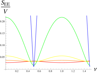
Figure 2: Plot of $S_{EE}/V$ against $\nu$, for $\alpha=0$ (red), $0.1$ (orange), $0.25$ (yellow), $1$ (green), $2$ (blue). Notice the periodicity and reflection symmetries.

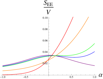
Figure 3: Plot of $S_{EE}/V$ against $\alpha$, for $\nu=0$ (red), $0.25$ (orange), $\nu_{c}=0.4062\dots$ (green), $0.43$ (blue) and $0.5$ (purple).

IV Discussion

In this letter, we have shown the calculation of the entanglement entropy for de Sitter space $\alpha$-vacua, by generalizing the analysis of Maldacena and Pimentel (2013). As is seen in Figure 2 and Figure 3, entanglement entropy increases significantly as we take $\alpha$ very large, for generic values of $\nu$. However only for $\nu=1/2$ and $3/2$, this tendency disappears. Note that $\nu=1/2$ is the conformal mass and $\nu=3/2$ is massless. It is interesting to understand more physically why such a mass dependence occurs.

Our calculation is done in the free scalar field. Therefore direct comparison with the holographic calculation for the Euclidean vacuum Maldacena and Pimentel (2013) is difficult. It must be interesting to ask how the calculation of entanglement entropy on the $\alpha$-vacua can be done in the strong coupling limit via holography, a la Ryu-Takayanagi formula Ryu and Takayanagi (2006). Understanding these will hopefully shed more light on the question of which vacuum one should choose in de Sitter space. We hope to come back to these question in near future.

Note added: Even though we have finished the calculation in this letter long before, we were working to include a holographic analysis. Then, a paper Kanno et al. (2014) appeared, which overlaps significantly to our work. Note that the result eq. (3.16) in Kanno et al. (2014) coincides with our results (III.2)-(27).