On the acceleration of spatially distributed agent-based computations:
a patch dynamics scheme

Abstract

In recent years, individual-based/agent-based modeling has been applied to study a wide range of applications, ranging from engineering problems to phenomena in sociology, economics and biology. Simulating such agent-based models over extended spatiotemporal domains can be prohibitively expensive due to stochasticity and the presence of multiple scales. Nevertheless, many agent-based problems exhibit smooth behavior in space and time on a macroscopic scale, suggesting that a useful coarse-grained continuum model could be obtained. For such problems, the equation-free framework [18, 16, 17] can significantly reduce the computational cost. Patch dynamics is an essential component of this framework. This scheme is designed to perform numerical simulations of an unavailable macroscopic equation on macroscopic time and length scales; it uses appropriately initialized simulations of the fine-scale agent-based model in a number of small “patches”, which cover only a fraction of the spatiotemporal domain. In this work, we construct a finite-volume-inspired conservative patch dynamics scheme and apply it to a financial market agent-based model based on the work of Omurtag and Sirovich [22]. We first apply our patch dynamics scheme to a continuum approximation of the agent-based model, to study its performance and analyze its accuracy. We then apply the scheme to the agent-based model itself. Our computational experiments indicate that here, typically, the patch dynamics-based simulation requires only $20\%$ of the full agent-based simulation in space, and need occur over only $10\%$ of the temporal domain.

, , , ,

1 Introduction

Over the last years agent-based modeling has become a powerful simulation technique for a number of applications, varying from ecology [4, 13, 5] to economics and financial systems [27, 28, 35], and from traffic and supply chain networks [14, 23, 33] to biological [6, 32, 36] and social [12, 15, 21] systems. Agents are treated as unique and discrete entities, allowing a straightforward way to incorporate detailed interactions between individuals via a set of microscopic rules. Modelers use the fine-scale evolution at the individual agent level to study the macroscopic, population level dynamical behavior, often referred to as emergent behavior. It would of course be desirable (and computationally much more efficient) to simulate this emergent behavior through a continuum macroscopic model. However, accurately accounting for the consequences of individual interactions at the macroscopic level can be highly nontrivial. As a consequence, accurate macroscopic equations are typically unavailable, even in cases when a clear separation of time scales strongly suggests that such equations should exist. In this work, we will consider a financial market agent-based model, in which a stochastic process describes the “motion” of an individual agent along a spatial domain representing the agent’s propensity to buy or sell. This stochastic process needs to be simulated for a large number of (interacting) agents over long times. Doing this over the entire spatiotemporal domain of interest to observe the relevant macroscopic variables (e.g., agent density) incurs a prohibitive computational cost.

The recently developed equation-free framework ([18, 16, 17]) can be applied to exploit the time-scale separation between the (fine-scale) individual dynamics and the (coarse-scale) population-level behavior by performing the expensive agent-based simulations in a grid of small patches, which cover only a fraction of the spatiotemporal domain. Exploiting smoothness, the solution for the entire region is approximated by repeated interpolation/extrapolation of the macroscopic variables recorded within these patches.

This framework is built around the central idea of a coarse time-stepper, which advances the coarse variables over a time interval of size $\delta t$. It consists of the following steps: (1) lifting, i.e., the creation of appropriate initial conditions for the microscopic model; (2) fine-scale evolution; and (3) restriction, i.e., the estimation of macroscopic observables from the fine-scale solution. This coarse time-stepper can subsequently be used as input for time-stepper-based “wrapper” algorithms performing macroscopic numerical analysis tasks. These include, for example, time-stepper based bifurcation codes to perform coarse bifurcation analysis for the unavailable macroscopic equation [30, 31, 34], and other system level tasks such as rare event analysis [19], control [2, 29] and optimization [3].

The patch dynamics scheme [17] is a combination of two sub-schemes - the gap-tooth scheme (interpolate macroscopic properties in space) [25] and the coarse projective integration scheme (extrapolate macroscopic properties in time) [24]. First, in the gap-tooth scheme [25], microscopic simulations are only performed in a number of small subdomains of the spatial domain (intervals for the case of one space dimension); in-between these patches lie what we call gaps. We continue the discussion for the one-space-dimension paradigm that fits our application. A coarse time-$\delta t$ map is then constructed as follows. We first choose a number of macroscopic grid points and a small interval (“tooth”)) around each grid point; we initialize the fine scale consistently with a macroscopic initial condition profile; apply the microscopic solver within each interval, using appropriate boundary conditions for time $\delta t$; and, finally, obtain macroscopic information at time $\delta t$ (e.g., by computing the average density in each tooth). In [25], the initial conditions for each of these teeth are obtained via interpolation over neighboring teeth; this can be seen to be equivalent to constructing a macroscopic finite difference approximation. In the gap-tooth scheme, this procedure is then repeated. We refer to [11] for an illustration of this scheme with particle-based simulations of the viscous Burgers equation.

Second, exploiting the smoothness of coarse variable evolution in the temporal domain, one can combine the gap-tooth scheme with a projective integration scheme [24]. In this context, we perform a number of gap-tooth steps of size $\delta t$ to obtain an estimate of the time derivative of the unavailable macroscopic equation. Based on this estimate, a projective step is subsequently taken over time $\Delta t\gg\delta t$. This combination has been termed patch dynamics [17].

In previous work, the gap-tooth and patch dynamics schemes have been applied to study a diffusion homogenization problem [25, 26], as well as a biological dispersal model [9]. For the kind of agent-based problems we study in this work, a conservation law needs to be satisfied. For this reason, instead of basing the gap-tooth scheme on a finite difference approximation, we design a finite volume-based patch dynamics scheme. We first apply this scheme to an approximate continuum model of the agent-based dynamics to illustrate the scheme, as well as to facilitate our error analysis. In this case, our “inner” microscopic model is a fine discretization of this continuum model, and our microscopic simulator is a classical finite volume scheme within each tooth. In general, a given microscopic code only allows us to run it with a set of predefined boundary conditions. It is highly non-trivial to impose macroscopically inspired boundary conditions on such microscopic codes, see, e.g. [20] for a control-based strategy. As in [26], the boundary conditions on the teeth are imposed via the use of buffer regions, surrounding the teeth, to “protect” the tooth inside each simulation unit from boundary artifacts. We call “simulation unit” the union of a tooth and its edge buffers. After several gap-tooth steps, we project the macroscopic properties forward in time for a bigger step $\Delta t$. Based on the projected macroscopic properties, we again construct consistent microscopic initial conditions for the simulation units and the cycle repeats. We study the performance of this patch dynamics scheme, and compute its order of accuracy both analytically and numerically. Subsequently, we apply the scheme to the agent-based model, and observe that, typically, this requires the expensive microscopic simulations in only $20\%$ of the spatial domain and $10\%$ of the temporal domain.

These micro/macro ideas also form the basis of the heterogeneous multiscale method [7, 8]. There, a macro-scale solver is combined with an estimator for quantities that are unknown because the macroscopic equation is not available. This estimator subsequently uses appropriately constrained runs of the microscopic model. For a recent overview of results obtained in that framework, we refer to [1].

The remainder of this paper is organized as follows: in section 2 we introduce an agent-based financial market model based on the work of [22] and the associated continuum approximation they derive. In section 3 we describe the “inner” finite volume scheme for the continuum model. In section 4 we describe the patch dynamics scheme. In section 5 we first present patch dynamics results using the discretization introduced in section 3 as the inner solver, and then analyze the order of consistency of this scheme both analytically and numerically. The main result, the agent-based patch dynamics computations, are also presented in section 5. We conclude with a brief summary and discussion in section 6.

2 The models

2.1 The agent-based model

We consider a financial market model initially described by Omurtag and Sirovich [22]. This model simulates the actions of buying and selling by a large population of $N$ interacting individuals in the presence of mimesis. In this model, the $i$-th agent’s propensity to buy or sell is indicated by its state $x_{i}(t)\in(-1,1)$ which evolves according to two coupled processes. The first process is the exponential decay, at constant rate $\gamma$, of $x_{i}(t)$ towards the neutral state $0$. This decay implies that each agent gradually forgets its current state and tends to eventually become neutral in its preference for buying or selling.

The second process is a stochastic process denoted by $I_{i}(t)$ which represents the effect of incoming information to each agent’s state $x_{i}(t)$. $I_{i}(t)$ incorporates three factors: (1) the arrival times of incoming information; (2) the type of this information (i.e., “good” or “bad”); and (3) the quantitative effect of this information on $x_{i}(t)$. The arrival of incoming information is assumed to follow a Poisson distribution with mean arrival frequency $(\nu^{+}+\nu^{-})$, where $\nu^{+}$ denotes the mean arrival frequency for good news and $\nu^{-}$ denotes the one for bad news. The mean arrival frequencies are given by

$$\nu^{\pm}=\nu_{ex}^{\pm}+gR^{\pm},$$ (1)

where the parameters $\nu_{ex}^{+}$ and $\nu_{ex}^{-}$ represent the contribution of external information each individual receives from its environment (e.g., mass media news or opinions of stock market consultants) and are assumed time-independent. The quantities $R^{+}$ and $R^{-}$ are the buy rates and sell rates, respectively, defined as the number of buys or sells happening in the market per unit time over a small finite time horizon (which we call reporting horizon) normalized by the total number of agents in the market. The parameter $g$ is a feedback constant which quantifies the extent to which the individuals’ propensity to buy or sell is determined by the buy and sell rates. Note that the buy and sell rates are collective properties of the population (i.e., all the agents in the market), which implies that the second term of (1), $gR^{\pm}$, embodies how each individual agent’s state is affected by the collective behavior of the entire population at that moment in time.

Each arriving “quantum” of information has probability $\nu^{+}/(\nu^{+}+\nu^{-})$ to be good news and $\nu^{-}/(\nu^{+}+\nu^{-})$ to be bad news. When good news arrives for agent $i$, the value of $x_{i}(t)$ is increased instantaneously - jumps - by a fixed amount $\epsilon^{+}>0$; similarly, when bad news arrives, $x_{i}(t)$ decreases instantaneously - jumps - changing by $\epsilon^{-}<0$. If, after a positive jump, the value of $x_{i}(t)$ exceeds the right boundary (i.e., $x_{i}(t)>1$), then a “buy” is considered to have occurred and the number of buys for that time interval is increased by one. Similarly, after $x_{i}(t)$ crosses the left boundary (i.e., $x_{i}(t)<-1$), the number of sells is increased by one. In either case, $x_{i}(t)$ is set back to the neutral state (i.e., $x_{i}(t)=0$ with a small random offset to prevent discontinuities) after the number of buys or sells is updated. In this way, each individual agent’s decision affects the population’s collective behavior. This discrete jump process, combined with the previously described exponential decay, form the evolutionary rule for each agent’s state $x_{i}(t)$, which can be summarized as the following stochastic differential equation

$$dx_{i}=-\gamma x_{i}(t)dt+dI_{i}(t).$$ (2)

2.2 The continuum model

It is possible to derive a concise approximate description of the dynamics of a large assembly of agents by keeping track of only the density $\rho(x,t)$ of agents at each state $x$, rather than the individual states of every agent in the population. The resulting approximate evolution equation for $\rho(x,t)$, averaged over a large number of replicas of the population, is given by [22]

$$\frac{\partial\rho}{\partial t}=-\gamma\frac{\partial{(x\rho)}}{\partial x}+\sum_{k=+,-}\nu^{k}(\rho(x-\epsilon^{k},t)-\rho(x,t))+(R^{+}+R^{-})\delta(x).$$ (3)

For small $\epsilon^{\pm}$ by expanding $\rho(x-\epsilon^{\pm},t)$ about $\rho(x,t)$ in terms of $\epsilon^{\pm}$ and truncating terms higher than second order in $\epsilon^{\pm}$, one obtains a Fokker-Planck-type approximation,

$$\frac{\partial\rho}{\partial t}=\frac{\partial}{\partial x}(\mu\rho)+\frac{1}{2}\sigma^{2}\frac{\partial^{2}\rho}{\partial x^{2}}+(R^{+}+R^{-})\delta(x)\,,$$ (4)

where

$$\mu(x,t)=\gamma x-(\nu^{+}\varepsilon^{+}+\nu^{-}\varepsilon^{-})\,,$$ (5)

and

$$\sigma^{2}(t)=\nu^{+}(\varepsilon^{+})^{2}+\nu^{-}(\varepsilon^{-})^{2}\,.$$ (6)

Because agents leave the domain at $x=\pm 1$ and are restored at the origin, we have $\rho(x=\pm 1,t)=0$, and a Dirac $\delta$ birth term at the origin. The buy and sell rates are defined as the outgoing fluxes at the boundaries, $R^{\pm}=\mp\frac{1}{2}\sigma^{2}\partial\rho/\partial x\mid_{x=\pm 1}$. The Fokker-Planck-type equation (4), with its non-local reinjection term, is the approximate continuum model in our study.

3 The finite volume scheme

We are now ready to describe a finite volume discretization of eq (4), which will serve as the first “inner” fine-scale simulator on which our exploratory patch dynamics scheme (described in section 4) will be based. We divide the one dimensional spatial domain into equal-sized grid cells and keep track of our approximations to the average densities in these cells. At each time step we update the average cell densities using approximations of the fluxes through the edges of the cells. As shown in Fig. 1, we denote the $i^{th}$ grid cell by

$$\it{C}_{i}=(x_{i-1},x_{i})\,;$$ (7)

Figure 1: Illustration of a finite volume scheme for updating the cell average $U_{i-1/2}^{n}$ by fluxes at the cell edges.

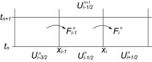
$U_{i-1/2}^{n}$ denotes the approximate average cell density in the $i$th cell at time $t_{n}$,

$$U_{i-1/2}^{n}\approx\frac{1}{\Delta x}\int_{x_{i-1}}^{x_{i}}\rho(x,t_{n})dx\equiv\frac{1}{\Delta x}\int_{\it{C}_{i}}\rho(x,t_{n})dx\,,$$ (8)

where $\Delta x=x_{i}-x_{i-1}$ denotes the size of the cell. Except for the central grid cell, which will be treated separately because of the particle reinjection, Eq. (4) can be rewritten as

$$\frac{\partial\rho}{\partial t}=\frac{\partial}{\partial x}(\mu\rho+\frac{1}{2}\sigma^{2}\frac{\partial\rho}{\partial x})\,.$$ (9)

Define the function $f(x,t)$ as the flux term

$$f(x,t)=-(\mu(x,t)\rho(x,t)+\frac{1}{2}\sigma^{2}(t)\frac{\partial\rho(x,t)}{\partial x})\,,$$ (10)

so that the integral form (in space) of Eq. (9) gives

$$\frac{d}{dt}\int_{\it{C_{i}}}\rho(x,t)dx=f(x_{i-1},t)-f(x_{i},t)\,.$$ (11)

Integrating Eq. (11) in time from $t_{n}$ to $t_{n+1}$ and dividing by $\Delta x$ gives

$$\frac{1}{\Delta x}\int_{\it{C}_{i}}\rho(x,t_{n+1})dx=\frac{1}{\Delta x}\int_{\it{C}_{i}}\rho(x,t_{n})dx-\frac{1}{\Delta x}\left[\int_{t_{n}}^{t_{n+1}}f(x_{i},t)dt-\int_{t_{n}}^{t_{n+1}}f(x_{i-1},t)dt\right]\,.$$

Based on Eq. (8), Eq. (3) can be rewritten as

$$U_{i-1/2}^{n+1}=U_{i-1/2}^{n}+\frac{\Delta t}{\Delta x}(F_{i-1}^{n}-F_{i}^{n})\,,$$ (12)

where $U_{i-1/2}^{n}$ is the average density defined in eq.(8), and $F_{i-1}^{n}$ and $F_{i}^{n}$ denote the average fluxes (i.e. fluxes averaged over $\Delta t$) across cell edges, that is,

$$F_{i-1}^{n}=\frac{1}{\Delta t}\int_{t_{n}}^{t_{n+1}}f(x_{i-1},t)dt~{}~{}\rm{and}~{}~{}F_{i}^{n}=\frac{1}{\Delta t}\int_{t_{n}}^{t_{n+1}}f(x_{i},t)dt.$$ (13)

Based on (10), the average fluxes over the time step are approximated by

$$F_{i-1}^{n} \approx \it{F}(U_{i-3/2}^{n},U_{i-1/2}^{n})$$ (14)

$$\approx -(\mu_{i-1}\frac{U_{i-3/2}^{n}+U_{i-1/2}^{n}}{2}+\frac{1}{2}\sigma^{2}\frac{U_{i-1/2}^{n}-U_{i-3/2}^{n}}{\Delta x}),$$

$$F_{i}^{n} \approx \it{F}(U_{i-1/2}^{n},U_{i+1/2}^{n})$$ (15)

$$\approx -(\mu_{i}\frac{U_{i-1/2}^{n}+U_{i+1/2}^{n}}{2}+\frac{1}{2}\sigma^{2}\frac{U_{i+1/2}^{n}-U_{i-1/2}^{n}}{\Delta x})\,.$$

For a detailed discussion about the construction of diffusion fluxes for finite volume schemes see [10]. The fluxes at the outer two boundaries are expressed as (recall that $x_{0}=-1$ and $x_{N}=1$)

$$F_{0}^{n}=-R^{-}\approx-\sigma^{2}\frac{U_{1/2}^{n}}{\Delta x}~{}~{}\rm{and}~{}~{}F_{N}^{n}=R^{+}\approx\sigma^{2}\frac{U_{N-1/2}^{n}}{\Delta x}.$$ (16)

We use an odd number of grid cells $N$ for this scheme. Since the central grid cell centered at $x_{N/2}$ contains the source point at $x=0$, two additional terms need to be added to Eq. (12) for this cell,

$$U_{N/2}^{n+1}=U_{N/2}^{n}+\frac{\Delta t}{\Delta x}(F_{(N-1)/2}^{n}-F_{(N+1)/2}^{n}+(R^{+}+R^{-}))\,.$$ (17)

Clearly, the above scheme is conservative by construction. In section 5, this scheme is used as the “inner” solver to mimic the agent-based simulator. Moreover, the associated patch dynamics scheme, introduced in the next section, will be inspired by this scheme, and will also be conservative at the agent level.

4 The patch dynamics scheme

Figure 2: Illustration of the gap-tooth scheme.

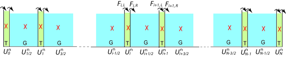
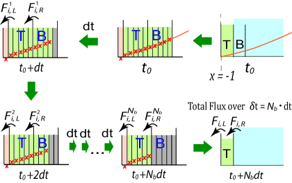
As mentioned previously, the patch dynamics scheme combines gap-tooth and projective integration schemes. The gap-tooth scheme is illustrated in Fig. 2. We have divided the one dimensional space into two kinds of unequal-sized grid cells: the narrower cells, which we call teeth, and the wider cells, which we call gaps. We intend to solve the microscopic model only within the teeth (plus some buffer regions to handle the teeth boundary conditions). However, we keep track of the average densities in both the teeth and the gaps to obtain a conservative scheme. As in the finite volume scheme, we want to update the average cell densities based on the fluxes at the edges of the cells,

$$U_{i}^{n+\delta} = U_{i}^{n}+\frac{\delta t}{L_{T}}(F_{i,L}^{n}-F_{i,R}^{n})\,,$$ (18)

$$U_{i+1/2}^{n+\delta} = U_{i+1/2}^{n}+\frac{\delta t}{L_{G}}(F_{i,R}^{n}-F_{i+1,L}^{n})\,,$$ (19)

where $L_{T}$ and $L_{G}$ denote the tooth and gap size respectively. However, in contrast to the finite volume scheme, the fluxes $F_{i,L}^{n}$ and $F_{i,R}^{n}$ are not computed based on a known macroscopic equation (which is usually not available for agent-based models). Instead, our goal is to compute these fluxes based on the “microscopic simulations” inside a small fraction of the spatial domain - the simulation unit (“$\alpha\Delta x$” shown in Fig. 3). These separated simulation units are the only locations where microscopic simulations take place. The numerical simulation of the microscopic model in each simulation unit provides information on the evolution of the global state at the spatial location of the simulation unit, as if we were running the microscopic simulations in the entire spatial domain. Therefore, it is crucial to choose appropriate boundary conditions, so that the solutions inside the teeth evolve as if the simulations were performed over the entire domain. For some cases it is possible to implement macroscopically-inspired constraints on the microscopic model as boundary conditions [25]. However, this is not always the case. To overcome this difficulty, as discussed in [26], we use a larger box - the simulation unit - to run the microscopic simulations, but still compute the flux used to update the macroscopic state at the teeth boundaries. Each simulation unit consists of one tooth and its edge buffers; the simulation units on the outer boundaries of the spatial domain are treated slightly differently, as discussed later. The purpose of the additional computational domains, the buffers, is to “protect” the teeth simulations from boundary artifacts. This can be accomplished over short enough time intervals, provided the buffers are large enough.

Figure 3: Illustration of the lifting procedure. (a) lifting procedure in the bulk of the domain. A local quadratic polynomial is constructed such that the averaged polynomial values inside the tooth (region 3), and inside the gaps (region 1 and 5) equal the average densities in these regions. (b) lifting procedure in the left boundary. (c) lifting procedure in the right boundary. One point value (zero on the the outer boundary) and two average values are used in constructing the local polynomials for the simulation units at the two boundaries.

As Fig. 2 shows, we divide the one-dimensional spatial domain into an odd number, $N$, of grid cells $\it{C_{i}},i=1,2,...,N$. The size of each cell is $\Delta x=2/N$. We then put teeth (narrow bins) at the edges of these cells and put gaps (wide bins) between the teeth. There are $\it{N+1}$ teeth and $\it{N}$ gaps. The average densities for the teeth at time $t_{n}$ are denoted as $U_{i}^{n},i=0,2,...N$, and the densities for the gaps are denoted as $U_{i-1/2}^{n},i=1,2,...N$. We want to update these macroscopic properties at time $t_{n+1}$ based on the microscopic simulations inside the simulation units during the time step from $t_{n}$ to $t_{n}+\delta t$.

The patch dynamics algorithm to proceed from $U_{i}^{n}$ to $U_{i}^{n+1}(i=0,\frac{1}{2},1,\cdots,N)$ is given below:

1. Lifting. At time $t_{n}$ create initial conditions $u^{i}(x,t_{n}),i=0,...N$ inside each simulation unit for the microscopic simulator, consistent with the spatial profile of the macroscopic properties - the average densities inside the teeth and gaps $U_{i}^{n}(i=0,1/2,1,...N)$.

2. Simulation. Based on the microscopic initial condition constructed in step 1 compute $F_{i,L}$ and $F_{i,R}$ by running the microscopic simulator inside the simulation units from time $t_{n}$ to $t_{n}+\delta t$.

3. Restriction. Obtain the spatially averaged densities inside the teeth and gaps $U_{i}^{n+\delta}(i=0,1/2,1,...N)$ based on Eq. (18)-(19).

4. Projective step. Estimate the macroscopic time derivative at time $t_{n}$, e.g., as

$$\mathcal{F}(U_{i}^{n};\delta t)=\frac{U_{i}^{n+\delta}-U_{i}^{n}}{\delta t}\,,$$ (20)

and use it in a time integration method of choice, e.g., forward Euler,

$$U_{i}^{n+1}=U_{i}^{n}+\Delta t\mathcal{F}(U_{i}^{n};\delta t)\,.$$ (21)

4.1 Lifting Procedure

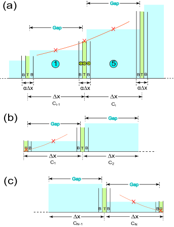
Except for the two outer teeth that receive special treatment, we create the microscopic initial condition inside the $\it{i^{th}}$ simulation unit by constructing a local quadratic polynomial approximation, $u^{i}(x,t)$, to the density that matches the average density in a tooth and its two neighboring gaps as follows. Let $H$ be the width of the tooth (so $\Delta x-H$ is the width of the gap) and require

$$\frac{1}{H}\int_{-H/2}^{H/2}u^{i}(x,t_{n})dx = U_{i}^{n},$$ (22)

$$\frac{1}{\Delta x-H}\int_{-\Delta x+H/2}^{-H/2}u^{i}(x,t_{n})dx = U_{i-1/2}^{n},$$ (23)

$$\frac{1}{\Delta x-H}\int_{H/2}^{\Delta x-H/2}u^{i}(x,t_{n})dx = U_{i+1/2}^{n}.$$ (24)

As shown in Fig. 3a, the microscopic initial conditions $u^{i}(x,t_{n})$ $(i=1,2,...N-1)$ are constructed such that the averaged function values inside the tooth (region 3), and inside the neighboring gaps (regions 1 and 5) equal the average densities in these regions.

At the two boundaries, as Fig. 3b and c show, there are gaps only on one side of the boundary teeth so the microscopic initial conditions are created in a slightly different manner. At the left boundary, a local quadratic polynomial $u^{0}(x,t_{n})$ is constructed such that

$$u^{0}(-1,t_{n}) = 0,$$ (25)

$$\frac{1}{H}\int_{-H/2}^{H/2}u^{0}(x,t_{n})dx = U_{0}^{n},$$ (26)

$$\frac{1}{\Delta x-3H/2}\int_{H/2}^{\Delta x-H}u^{0}(x,t_{n})dx = U_{1/2}^{n}.$$ (27)

Similarly, at the right boundary a local quadratic polynomial $u^{N}(x,t_{n})$ is constructed such that

$$u^{N}(1,t_{n}) = 0,$$ (28)

$$\frac{1}{H}\int_{-H/2}^{H/2}u^{N}(x,t_{n})dx = U_{N}^{n},$$ (29)

$$\frac{1}{\Delta x-3H/2}\int_{-\Delta x+H}^{-H/2}u^{N}(x,t_{n})dx = U_{N-1/2}^{n}.$$ (30)

Note that the left edge of the leftmost tooth (and similarly the right edge of the rightmost tooth) is put at the two boundaries $x=\pm 1$, instead of their respective centers. For this reason, the outermost gaps are of a slightly different size ($\Delta x-\frac{3}{2}H$) compared to the inner ones (which are of equal size $\Delta x-H$).

4.2 Simulation step

As mentioned previously, for our initial experiment and its analysis a fine-grid finite volume scheme is first used as the“inner”, microscopic simulator. We emphasize again that the purpose of first using a fine discretization of eq (4) as our “inner” microscopic solver is to facilitate a numerical study of the errors involved - something we cannot do when dealing directly with the agent-based simulator.

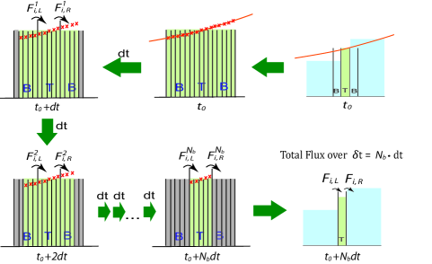
We divide each simulation unit into $N_{t}+2N_{b}$ fine bins, where $N_{t}$ denotes the number of fine bins inside the tooth while $N_{b}$ denotes the number of fine bins inside each buffer. All these fine bins are of equal size $\delta x$. Based on the previously constructed local quadratic polynomial $u^{i}(x,t_{n})$ we initialize the averaged densities in the fine bins as follows:

$$\frac{1}{h}\int_{x_{j}-h/2}^{x_{j}+h/2}u^{i}(x,t_{n})dx=u_{j}^{i}\,,\\$$ (31)

where $x_{j}$ denotes the center of each fine bin and $u_{j}^{i}$ denotes the average densities inside the $j^{th}$ fine bin of the $i^{th}$ simulation unit (as the red cross marks in Fig. 4 and 5 denote). Fig. 4 illustrates the simulation step in the bulk of the spatial domain. Starting from the previously constructed local quadratic polynomial, we first initialized the average densities inside the fine bins using Eq. (31). To evolve $u_{j}^{i}(t_{0})$ for one microscopic step $dt$, as Eq. (12) and (14-15) show, it requires $u_{j-1}^{i}(t_{0})$, $u_{j}^{i}(t_{0})$ and $u_{j+1}^{i}(t_{0})$. Because of that, we are not able to evolve the solutions for the two bins at the boundaries (the two bins denoted in grey in the upper-left part of Fig. 4). Therefore, after the first microscopic time step $dt$, these two bins are discarded. For the same reason, after another microscopic time step dt, two more (now outer) fine bins need to be discarded, and so on until all the bins in the buffer regions are discarded. There are $N_{b}$ fine bins in each buffer, so we can run the microscopic simulator for $N_{b}$ microscopic time steps. During the $k$-th step ($k=1,2,...N_{b}$), we save the fluxes computed at the left (resp. right) edge of the $i$-th tooth, $F_{i,L}^{k}$ (resp.  $F_{i,R}^{k}$).

The simulations in the leftmost and rightmost simulation units are performed slightly differently. As Fig. 5 shows, a buffer is only used on one side of the tooth (the side to the interior of the spatial domain). On the other side, the outer boundary of the spatial domain, the boundary condition $\rho(x=\pm 1)=0$ needs to be enforced. This is achieved using a ghost bin (colored pink in Fig. 5) with density equal in magnitude but opposite in sign to the density of the leftmost (resp. rightmost) inner bin. (See Fig. 5 for an illustration of the left boundary; the right boundary is treated in a similar way.)

Figure 4: Illustration of the simulation step for the simulation units in the bulk of the spatial domain.

Figure 5: Illustration of the simulation step for the simulation unit at the left boundary.

4.3 Restriction procedure

At the end of the $N_{b}^{th}$ step, we update the total fluxes at the edges of each tooth for the coarse time interval $\delta t=N_{b}\cdot dt$ as follows

$$F_{i,L} = \frac{1}{N_{b}}\sum_{k=1}^{N_{b}}F_{i,L}^{k},$$ (32)

$$F_{i,R} = \frac{1}{N_{b}}\sum_{k=1}^{N_{b}}F_{i,R}^{k}.$$ (33)

Then, based on Eqn. (18 - 19), the coarse variables - the average densities inside the teeth and gaps $U_{i}^{n+\delta}(i=0,1/2,1,...N)$ - are updated.

4.4 Projective step

Eq. (20) is now used to estimate the macroscopic time derivative and Eq. (21) is used to project the macroscopic solutions forward to obtain $U_{i}^{n+1}$.

5 Results and discussion

5.1 Comparison of the patch-dynamics scheme with fine and coarse finite volume schemes for the continuum equation

We compare the performance of the patch-dynamics scheme with two other schemes: one is the fine grid finite volume scheme i.e., our microscopic simulator applied to the entire region; the other is a coarse grid finite volume scheme, which mimics the usually unavailable macroscopic solver. All three schemes are first applied to the continuum approximation of the agent-based model.

Figure 6: Comparison of the solutions obtained using the three different schemes. (a) The initial conditions for the three schemes, which are constructed from a common Gaussian-like function $f(x)=a\cdot exp\left(-\left(\left(x-b\right)/c\right)^{2}\right)$ with $a=1.811,b=0.01545,c=0.3115$. (b) Solutions of the three schemes at time $4\times 10^{3}\Delta t$. (c) Comparison of the errors of the patch-dynamics scheme and the coarse finite volume scheme at time $4\times 10^{3}\Delta t$, using the fine finite volume scheme as the reference. (d) Steady state solutions. (e) Comparison of the errors of the patch-dynamics scheme and the coarse finite volume scheme at steady state. The blue curve (in (a), (b), and (e)) denotes the solution of the fine finite volume scheme; the red curve (in (a), (b), and (e)) denotes the solution of the coarse finite volume scheme; the blue dots (in (a), (b), and (e)) denote the solutions of the teeth for the patch dynamics scheme; the blue dots (in (c) and (e)) denote the errors (in teeth) of the patch dynamics scheme; The red cross marks in (in (c) and (e)) denote the errors of the coarse finite volume scheme. Parameter values for the three schemes are as follows: $g=40,\epsilon^{+}=0.075,\epsilon^{-}=-0.072,\gamma=1,\nu_{ex}^{+}=\nu_{ex}^{-}=20$. Parameters specific for the patch dynamics scheme: $\alpha=0.1,N=41,N_{b}=N_{t}=10,dt=4h^{2},\delta t=9dt,M=90,\Delta t=(M+1)\delta t$. Parameters specific to the coarse finite volume scheme: $N=41,\Delta t=(M+1)\delta t$. Parameters specific to the fine finite volume scheme: $N_{fine}=1271$.

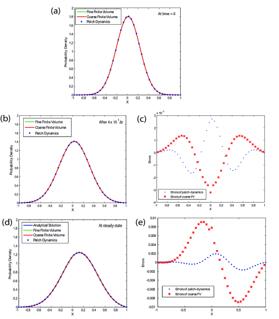
Fig. 6 shows several snapshots of the solutions of these three schemes along the time-path towards their steady states. Starting from the same Gaussian-like initial conditions (Fig. 6a) we evolve the solutions of the three systems for a long time (Fig. 6b shows one snapshot of the transient solutions) until they have reached their steady states (Fig. 6d). As we can see from the figure, the solution of the patch-dynamics scheme agrees well with the other two schemes along the entire process. The steady state solutions of the three schemes also agree well with the analytical steady state solution of the problem (Fig. 6d). In Fig. 6c and 6e we plot the differences between the fine finite-volume scheme and the other two methods, patch dynamics and coarse finite volume scheme. The solution to the fine finite-volume scheme is an approximation to the true solution, so these differences can be viewed as a first approximation to the errors in the other two methods. Also, since the patch dynamics uses the fine finite-volume scheme as its microscopic solver, the differences between it and patch dynamics are an indication of the error introduced by the patch dynamics scheme. As we can see from Fig. 6c and 6e, during the transient phase the two schemes give comparable errors, while as we further evolve the system to steady state the patch dynamics scheme gives smaller errors. This is probably due to the fact that our patch dynamics scheme utilizes more microscopic level information.

We now turn to the computational savings of patch dynamics. For the patch-dynamics scheme, we divide the spatial domain into $N=41$ big cells, giving 42 teeth and 41 gaps. We run “microscopic simulations” in only $\alpha=10\%$ of the spatial domain (since the width of each simulation unit is equal to only $10\%$ of each big cell). Inside each simulation unit we put $10$ equal-sized fine bins inside each tooth and each buffer to run the microscopic simulations (mimicked here by the fine grid finite volume scheme). We use $dt=4\times h^{2}$ as the time step for the microscopic simulator ($\delta x$ is the width of the “fine” bin). After running the microscopic simulator for $n_{b}=10$ microscopic steps (dt), or equivalently one coarse time step $\delta t=n_{b}\times dt$, we project macroscopic variables 90 coarse steps forward in time. This means that the microscopic simulations are performed in only $1.11\%$ of the temporal domain. For the fine finite volume scheme, we use $N_{fine}=1271$ fine bins, and use the same time step size dt as the one used in the microscopic simulator for the patch dynamics scheme. For the coarse finite volume scheme we use the same number of big cells ($N=41$) as the one used for the patch-dynamics scheme. The time step size of this scheme is set to be equal to the effective time step size $\Delta t$ of the patch dynamics scheme (recall that $\Delta t=(M+1)\delta t$, with $M=90$). Overall, in this illustrative example the patch dynamics scheme runs the microscopic simulations in only $10\%$ of the spatial domain and $1.11\%$ of the temporal domain.

5.2 Error Analysis

The patch-dynamics scheme uses a microscopic integrator that is not specified (in this paper we have used an agent-based model as well as a fine-scale finite volume method to illustrate the method and to permit better analysis). The purpose of the gap-tooth part of the scheme is to estimate time derivatives of the macroscopic tooth and gap densities (more precisely, the chords of their time-dependent solutions over a small interval $\Delta t$), and these are input to an unspecified outer integrator or other macroscopic numerical analysis procedure (in this paper we have used projective forward Euler integration, but any scheme could be used).

The errors thus arise from three sources: the microscopic integrator itself, the patch-dynamics scheme, and the outer integrator (or whatever other numerical procedure we apply to the chord estimates). The final error is a non-linear combination of the errors from all three sources that depends on details of the problem being solved and the details of each method, making it very difficult to isolate each part of the process. Hence it seems advisable to consider each step from a backward error perspective. In the backward error view, the microscopic integrator integrates a perturbed equation exactly. The size of the perturbation is a function of the microscopic integrator and the equation being integrated, but for our purposes we can ignore it and assume that the microscopic integrator is exact (it is for the perturbed equation). Then we can examine the size of the errors introduced by the gap-tooth scheme.

The equations for estimating the teeth and gap chord slopes (for other than the center and end teeth) are:

$$\frac{U_{i}^{n+1}-U_{i}^{n}}{\Delta t}=\frac{F_{i,L}^{n}-F_{i,R}^{n}}{H}$$ (34)

and

$$\frac{U_{i-1/2}^{n+1}-U_{i-1/2}^{n}}{\Delta t}=\frac{F_{i-1,R}^{n}-F_{i,L}^{n}}{\Delta x-H}\,.$$ (35)

Note that if we compute the fluxes $\{F_{i,L}^{n}\}$ and $\{F_{i,R}^{n}\}$ exactly, these equations are exact. If, for example, we ran the microscopic integrator over all space and time, these equations would give the exact values of the average teeth and gap densities over time. However, we introduced the teeth to avoid running the microscopic simulation over all of space, so that after a finite time the buffer regions fail to “protect” the teeth from the lack of simulation information from the bulk of the gaps. At that point we have to stop the microscopic integration, and lift from the macroscopic information using the process described in Section 4 to get a new microscopic description. Under the assumption that the microscopic integrator is correct, the error introduced by the patch dynamics scheme is simply a change of initial values at the start of the $\Delta t$ integration block.

In the next subsection we will examine this error analytically and then report on some computational estimates of the errors in our finance model in the following subsection.

5.2.1 Lifting Error

Suppose that the computed microscopic solution at $t_{n}$ is $v(x)$. For each tooth the lifting process creates a quadratic polynomial approximation, $u(x)$, such that the average densities of $u$ and $v$ agree in the tooth and its neighboring gaps. The microscopic integration then continues starting from the $u$ values rather than from $v$. The effect is to add

$$r(x)=u(x)-v(x)$$ (36)

to the initial values for the next integration interval.

We analyze each tooth separately. Let us set the spatial origin, $x=0$, to be the tooth center and assume that the Taylor series for $v(x)$ is

$$v(x)=v_{0}+v_{1}x+v_{2}x^{2}/2+v_{3}x^{3}/6+\cdots,$$ (37)

i.e., $v_{q}$ is the $q$-th spatial derivative of $v(x)$. It will be convenient to define $h=H/2$ and $D=\Delta x-h$ (so the left and right gaps are $[-D,-h]$ and $[h,D]$. Because of the average density condition in the tooth and its surrounding gaps we have

$$\int_{-D}^{-h}r(x)dx = 0,$$

$$\int_{-h}^{h}r(x)dx = 0,$$ (38)

$$\int_{h}^{D}r(x)dx = 0,$$

where $r(x)$ is given in eq (36). Let us define $u(x)$ as

$$u(x)=r_{0}+v_{0}+(r_{1}+v_{1})x+(r_{2}+v_{2})x^{2}/2.$$ (39)

Hence

$$r(x)=u(x)-v(x)=r_{0}+r_{1}x+r_{2}x^{2}/2-v_{3}x^{3}/6-v_{4}x^{4}/24+\cdots$$

Solving eq (38) for $r_{i}$ in terms of $v_{j}$ we get

$$r_{0} = -D^{2}h^{2}v_{4}/120+{\rm O}(D^{6}+h^{6}),$$ (40)

$$r_{1} = (D^{2}+h^{2})v_{3}/24+{\rm O}(D^{4}+h^{4}),$$ (41)

$$r_{2} = (D^{2}+h^{2})v_{4}/20+{\rm O}(D^{4}+h^{4}).$$ (42)

Thus, over the region comprising the tooth and its neighboring gaps the largest error that can be introduced is

$$E=\max_{x\in[-D,D]}|[(D^{2}+h^{2})x-4x^{3}]v_{3}/24|+{\rm O}(h^{4}+D^{4})$$ (43)

which is ${\rm O}(h^{3}+D^{3})$.

How does the error in Eq. 43 affect the solution of the integration problem? Unfortunately it depends on the problem, but if the problem is such that modest perturbations do not cause serious difficulties (for example, if the system after semi-discretization in space satisfies a Lipschitz condition) the final error is equal to the sum of the errors, each multiplied by bounded amplifications. Thus, if the number of steps in the outer integrator is ${\rm o}((\max(D,h)^{-3})$, the global error will be bounded. If the average time step size is ${\rm O}((\max(D,H))^{2})$ the global error is ${\rm O}(\max(D,H))$ over any finite interval, and if the average time step size is ${\rm O}(\max(D,H))$ the global error is ${\rm O}((\max(D,H))^{2})$. If the solution tends to a stable stationary state, then the final error may reflect only the most recent lifting errors and if many of the components are stiff, this may be true over much of the integration interval.

5.2.2 Numerical Results

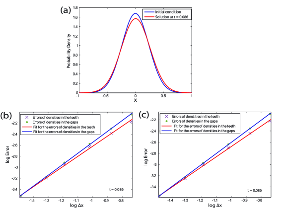
To numerically validate that the order of consistency for the patch dynamics scheme is two, we compare solutions of the patch-dynamics scheme (using a fine-grid finite volume scheme as the “inner” microscopic simulator) with the solutions of a reference scheme, which is also a fine-grid finite volume scheme (but over the entire physical domain). In this reference scheme, the spatial domain is divided into $963$ fine bins with bin width $\delta x=2/963$. The microscopic time step is set to be $dt=2\delta x^{2}$. As Fig. 7a shows, starting from the same Gaussian-like initial condition, we evolve both the patch-dynamics scheme and the reference scheme for some time ($t=0.086$, or equivalently $10000$ time steps in the reference scheme), and then compute the differences between the solutions of these two schemes in order to construct the subsequent log-log plot for the consistency order analysis.

For the patch-dynamics scheme, two distinct limits have been numerically simulated. The first limit corresponds to cases where the tooth size becomes very small. In practice, the tooth size in this limit is set to be equal to the fine bin size in the reference scheme ($\delta x=2/963$). The size of the buffers is set to be the same as the one of the teeth. By fixing the size of the teeth and buffers, we studied cases with different sizes of big cells and therefore different sizes of gaps. Recall that, as Fig. 3 shows, each big cell is of size $\Delta x$, which is equal to the sum of the sizes of a pair of tooth and gap. In the second limit, instead of fixing the teeth size to have a very small value, we keep the ratio between the sizes of the simulation unit and the big cell fixed, while varying both of them simultaneously. The second limit is closely related to the envisioned practical simulation cases, because in practice we need to use teeth with some finite size, in order to capture meaningful macroscopic properties.

For each limit we compute the differences between the average densities inside the teeth and the gaps for the patch dynamics scheme on the one hand, and the average densities inside the corresponding regions of the reference scheme on the other. We define the errors for the teeth and gaps as the L2 norm of these differences:

$$\left\|U_{t}-U_{ref}\right\| = \sqrt{\frac{1}{N+1}\sum_{i=0}^{N}(U_{t}^{i}-U_{ref}^{i})^{2}}$$ (44)

$$\left\|U_{g}-U_{ref}\right\| = \sqrt{\frac{1}{N}\sum_{j=1/2}^{N-1/2}(U_{t}^{j}-U_{ref}^{j})^{2}}$$ (45)

where, $U_{t}^{i}$ and $U_{g}^{j}$ denote the average densities in the teeth and gaps for the patch-dynamics scheme, while $U_{ref}^{i}$ and $U_{ref}^{j}$ denote the average densities inside the corresponding regions of the reference scheme. The detailed results of the different cases in these two limits are shown in Table 1.

To estimate the order of consistency, we generated the log(error) v.s. log($\Delta x$) plot and performed linear fitting. The fitted plots for the two limits are shown in Fig. 7 (b) and (c). The slope of the fitted lines together with their respective $95\%$ confidence interval estimates are shown in Table 2. The numerical consistency order estimates are all close to $2$; the slight deviation is most likely due to the discontinuity at the origin and the boundary conditions.

Figure 7: (a) The blue curve corresponds to the Gaussian-like initial condition for both the patch-dynamics scheme and the reference scheme. The red curve corresponds to the solution of the reference scheme at $t=0.086$. This was obtained by running the reference scheme for $10000$ time steps. The patch-dynamics scheme was running for the same amount of time. The differences of the average densities inside the teeth as well as the gaps between these two schemes were taken at this time point to generate the log-log plots. The model parameters used in these simulations are the same as the ones listed in Fig. 6. (b) Log(Error) v.s. log ($\Delta x$) plot for Limit 1. (b) Log(Error) v.s. log ($\Delta x$) plot for Limit 2. In (b) and (c), the dots denote the log(Error) v.s. log($\Delta x$) data points for the teeth, while the cross marks denote the corresponding data points for the gaps. The blue and red curves denote the linear fit for the data sets of the teeth and gaps respectively. The R-square values for the fits are all very close to one (0.998 and above). The slopes of the fitted lines (order of consistency estimates) together with their respective $95\%$ confidence intervals are presented in Table 2.

		Limit 1		Limit 2
N	$\Delta x$	$\left\|U_{t}-U_{ref}\right\|$	$\left\|U_{g}-U_{ref}\right\|$	$\left\|U_{t}-U_{rEf}\right\|$	$\left\|U_{g}-U_{rEf}\right\|$
$11$	$1.82E-1$	$6.76E-03$	$9.12E-03$	$6.03E-03$	$8.13E-03$
$15$	$1.33E-1$	$4.07E-03$	$5.01E-03$	$3.63E-03$	$4.47E-03$
$21$	$9.52E-2$	$2.29E-03$	$2.63E-03$	$2.04E-03$	$2.29E-03$
$31$	$6.45E-2$	$1.15E-03$	$1.20E-03$	$1.00E-03$	$1.07E-03$
$41$	$4.88E-2$	$6.61E-04$	$6.92E-04$	$5.75E-04$	$6.17E-04$
$61$	$3.28E-2$	$2.88E-04$	$3.02E-04$	$2.69E-04$	$2.75E-04$

Table 1: Numerical results of the consistency order analysis for the two limits. N is the number of big cells in the patch-dynamics scheme. $\Delta x$ denotes the size for the big cells. The error terms are defined in Eq. (44-45).

	Limit 1	Limit 2
$U_{t}$	1.839 (1.715, 1.964)	1.818 (1.732, 1.903)
$U_{g}$	1.991 (1.939, 2.043)	1.974 (1.948, 2.001)

Table 2: Consistency order estimates for the two limits. $95\%$ confidence intervals for the order estimates are shown in the brackets.

5.3 Patch dynamics scheme for the agent-based model

Finally, we turn to the agent-based model (discussed in section 2.1) for which the patch dynamics scheme has been designed. We divide the spatial domain into $N=21$ big cells, and set the ratio of the size of the simulation unit to the big cell ($\alpha$) to 0.2. This means we are running the microscopic simulations in $20\%$ of the spatial domain. Our macroscopic observables (our coarse variables) are the average agent densities inside the teeth and gaps. Inside each simulation unit the tooth and the two buffers are of equal size, and each of them has been subdivided into 10 fine bins. Based on the lifting procedure discussed in section 4.1, microscopic agent densities are assigned to these fine bins. We then convert these density values into numbers of agents based on the total amount of agents available in the system; in this case the total number of agents we use is $N_{agents}=3\times 10^{6}$. Once the number of agents for each fine bin is assigned we start the agent-based simulations. As illustrated in section 4.2, the coarse time step size $\delta t$ - the time we can run the agent-based simulator before we stop for reconstruction - is closely related to the size of the buffers. This is because the buffers are gradually “contaminated” due to boundary artifacts; we need to stop a little before these artifacts get propagated to the tooth. Our coarse time step size $\delta t$ is chosen to be $2\times 10^{-3}$. Within this time interval, the chance for any agent to travel a distance of the size of a buffer or more is very low. In this way agents outside each simulation unit will not affect the solution of the tooth (although they do affect the solution of the buffers), and the tooth is therefore protected. Along the simulation process, the fluxes of agents across the edges of the teeth are tracked. In section 4.2, the fluxes are updated based on equations of the artificial microscopic simulator (a PDE). In the agent-based case we track the fluxes by counting the number of agents going across those edges.

Due to the stochastic nature of the agent-based modeling, we also need to reduce the noise for the macroscopic variables. The agent-based simulations are therefore repeated inside each simulation unit for $N_{realizations}=20$ copies before the restriction procedure is applied. At the end of each coarse time step, we perform the restriction procedure to compute the averaged fluxes at the edges of the teeth. Based on these fluxes we update the numbers of agents inside the teeth as well as the neighboring gaps, and compute the corresponding densities based on the numbers of agents. Following the same procedure discussed in section 4.4, based on the macroscopic solutions (the densities) at the start and the end of each coarse time step, we estimate local time derivatives of the macroscopic variables and project them forward in time. What allows us to do this is the smoothness of these coarse variables in the time domain. In this case, we run the agent-based simulations over the duration of one coarse time step, and then “jump” nine coarse time steps ahead. In other words, we are running the agent-based simulations over $10\%$ of the temporal domain.

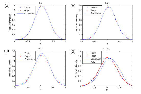
Fig. 8 shows four snapshots along a patch dynamics agent-based trajectory on its way to the eventual steady state. The solutions for the agent-based patch-dynamics simulations are plotted in blue (teeth) and red (gaps) respectively. To compare the performance, the solutions of a fine-grid finite volume scheme for the continuum model are also plotted (in blue curve)as a reference. The analytical steady state for the continuum model is shown in Fig. 8(d). Overall, the solutions of the agent-based patch-dynamics simulations match well (although not perfectly) with the solutions of the continuum model. The deviations are most likely due to the approximations made to derive the continuum model from the agent-based one. In Fig. 8(d) we can see that the steady state of the patch-dynamics agent based simulations matches the stationary state of the full scale agent-based simulations better than the analytical steady state of the continuum model matches it.

We reiterate that the patch-dynamics agent-based simulations require the “expensive” agent-based computations to be performed in only $10\%$ of the temporal domain and $20\%$ of the spatial domain compared to the full scale agent-based simulations.

Figure 8: Snapshots along a patch dynamics agent-based trajectory on its way to an eventual steady state. The average agent densities inside the teeth are denoted by red dots, while the ones inside the gaps are denoted by blue dots. To compare the performance, solutions of a fine-grid ($N=629$) finite volume scheme for the continuum model are plotted in (a-c) in blue curves. In (d) the analytical steady state of the continuum model is plotted as a blue curve while the approximated steady state of the full agent-based simulations is plotted as a red curve. Parameter values for the patch dynamics scheme are as follows: $N=21$, $\alpha=0.2$, $g=1$, $\epsilon^{+}=2.9\times 10^{-3}$, $\epsilon^{-}=-2.89\times 10^{-3}$, $\gamma=1\times 10^{-3}$, $N_{agents}=3\times 10^{6}$, $N_{realizations}=20$, $\delta t=2\times 10^{-3}$, $M=9$.

6 Conclusions

We described a patch dynamics scheme for conservative agent-based problems. This scheme approximates an unavailable effective equation over macroscopic time and length scales, when only a microscopic agent-based simulator is given. It only uses appropriately initialized simulations of the agent-based model over small subsets (patches) of the spatiotemporal domain, thus significantly reducing the computational cost. Because this scheme mimics a finite volume scheme for the underlying effective equation, it is conservative by construction. Since it is often not possible to impose macroscopically inspired boundary conditions on a microscopic agent-based simulation, we have used buffer regions around the patches, which temporarily shield the internal region of the patches from boundary artifacts. We have explored numerical characteristics of the scheme based on the continuum approximation (a Fokker-Planck-type evolution equation) of the agent-based model, and demonstrated its effectiveness for agent-based computations involving a financial market agent-based model. In this paper the agent-based model was mainly used for illustration purposes, to demonstrate the effectiveness of the approach. Several factors that can affect the performance of the patch dynamics scheme still need to be explored in more detail. One of the most interesting ones to study should be the effect of the noise (in the teeth and the gaps) on the estimation of relevant quantities, and through them to the overal performance of this scheme.

Acknowledgements. This work was partially supported by the US Department of Energy and the National Science Foundation.

References

- [1] A. Abdulle, W. E, B. Engquist, and E. Vanden-Eijnden. The heterogeneous multiscale method. Acta Numerica, 211–87, 2012
- Armaou et al. [2004] A. Armaou, C. I. Siettos, and I. G. Kevrekidis. Time-steppers and ’coarse’ control of distributed microscopic processes. International Journal of Robust and Nonlinear Control, 14(2):89–111, 2004.
- Bindal et al. [2006] A. Bindal, M. G. Ierapetritou, S. Balakrishnan, A. Armaou, A. G. Makeev, and I. G. Kevrekidis. Equation-free, coarse-grained computational optimization using timesteppers. Chemical Engineering Science, 61(2):779–793, 2006.
- Blanchart et al. [2009] E. Blanchart, N. Marilleau, J. L. Chotte, A. Drogoul, E. Perrier, and C. Cambier. Sworm: an agent-based model to simulate the effect of earthworms on soil structure. European Journal of Soil Science, 60(1):13–21, 2009.
- Buhl et al. [2006] J. Buhl, D. J. T. Sumpter, I. D. Couzin, J. J. Hale, E. Despland, E. R. Miller, and S. J. Simpson. From disorder to order in marching locusts. Science, 312(5778):1402–1406, 2006.
- Castiglione et al. [2007] F. Castiglione, F. Pappalardo, M. Bernaschi, and S. Motta. Optimization of haart with genetic algorithms and agent-based models of hiv infection. Bioinformatics, 23(24):3350–3355, 2007.
- E et al. [2003] W. E, B. Engquist, and Z. Y. Huang. Heterogeneous multiscale method: A general methodology for multiscale modeling. Physical Review B, 67(9), 2003. Times Cited: 1.
- E et al. [2007] W. E, B. Engquist, X. Li, W. Ren, and E. Vanden-Eijnden. Heterogeneous multiscale methods: A review. Communications in Computational Physics, 2(3):367–450, 2007. Times Cited: 68.
- Erban et al. [2006] R. Erban, I. G. Kevrekidis, and H. Othmer. An equation-free computational approach for extracting population-level behavior from individual-based models of biological dispersal Physica D, 2(215):1-24, 2006.
- Gassner et al. [2007] G. Gassner, F. Lorcher, and C. Munz. A contribution to the construction of diffusion fluxes for finite volume and discontinous galerkin schemes. Journal of Computational Physics, 224(2):1049–1063, 2007.
- Gear et al. [2003] C. W. Gear, J. Li, and I. G. Kevrekidis. The gap-tooth method in particle simulations. Physics Letters A, 316(3-4):190–195, 2003.
- Hamill and Gilbert [2009] L. Hamill and N. Gilbert. Social circles: A simple structure for agent-based social network models. JASSS-The Journal of Artificial Societies and Social Simulation, 12(2), 2009.
- Hellweger and Bucci [2009] F. L. Hellweger and V. Bucci. A bunch of tiny individuals-individual-based modeling for microbes. Ecological Modelling, 220(1):8–22, 2009.
- Ilie-Zudor and Monostori [2009] E. Ilie-Zudor and L. Monostori. Agent-based framework for pre-contractual evaluation of participants in project-delivery supply-chains. Assembly Automation, 29(2):137–153, 2009.
- Janssen et al. [2008] M. A. Janssen, L. N. Alessa, M. Barton, S. Bergin, and A. Lee. Towards a community framework for agent-based modelling. JASSS-The Journal of Artificial Societies and Social Simulation, 11(2), 2008.
- Kevrekidis and Samaey [2009] I. G. Kevrekidis and G. Samaey. Equation-free multiscale computation: Algorithms and applications. Annual Review of Physical Chemistry, 60:321–344, 2009.
- Kevrekidis et al. [2003] I. G. Kevrekidis, C. W. Gear, J. M. Hyman, P. G. Kevrekidis, O. Runborg, and C. Theodoropoulos. Equation-free coarse-grained multiscale computation: enabling microscopic simulators to perform system-level analysis. Comm. Math. Sciences, 1(4):715–762, 2003.
- Kevrekidis et al. [2004] I. G. Kevrekidis, C. W. Gear, and G. Hummer. Equation-free: The computer-aided analysis of complex multiscale systems. AIChE Journal, 50(7):1346–1355, 2004.
- Kopelevich et al. [2005] D. I. Kopelevich, A. Z. Panagiotopoulos, and I. G. Kevrekidis. Coarse-grained kinetic computations for rare events: Application to micelle formation. Journal of Chemical Physics, 122(4), 2005.
- Li et al. [1998] J. Li, D. Liao, and S. Yip. Imposing field boundary conditions in md simulation of fluids: optimal particle controller and buffer zone feedback. Mat. Res. Soc. Symp. Proc., 538:473–478, 1998.
- Nishizaki et al. [2009] I. Nishizaki, H. Katagiri, and T. Oyama. Simulation analysis using multi-agent systems for social norms. Computational Economics, 34(1):37–65, 2009.
- Omurtag and Sirovich [2006] A. Omurtag and L. Sirovich. Modeling a large population of traders: Mimesis and stability. Journal of Economic Behavior & Organization, 61(4):562–576, 2006.
- Pan et al. [2009] A. Pan, S. Y. S. Leung, K. L. Moon, and K. W. Yeung. Optimal reorder decision-making in the agent-based apparel supply chain. Expert Systems with Applications, 36(4):8571–8581, 2009.
- Rico-Martinez et al. [2004] R. Rico-Martinez, C. W. Gear, and I. G. Kevrekidis. Coarse projective kmc integration: forward/reverse initial and boundary value problems. Journal of Computational Physics, 196(2):474–489, 2004.
- Samaey et al. [2005] G. Samaey, D. Roose, and I. G. Kevrekidis. The gap-tooth scheme for homogenization problems. Multiscale Modeling & Simulation, 4(1):278–306, 2005.
- Samaey et al. [2006] G. Samaey, I. G. Kevrekidis, and D. Roose. Patch dynamics with buffers for homogenization problems. Journal of Computational Physics, 213(1):264–287, 2006.
- Samanidou et al. [2007] E. Samanidou, E. Zschischang, D. Stauffer, and T. Lux. Agent-based models of financial markets. Reports on Progress in Physics, 70(3):409–450, 2007.
- Shimokawa et al. [2007] T. Shimokawa, K. Suzuki, and T. Misawa. An agent-based approach to financial stylized facts. PHYSICA A-Statistical Mechanics and its Applications, 379(1):207–225, 2007.
- Siettos et al. [2006a] C. I. Siettos, I. G. Kevrekidis, and N. Kazantzis. An equation-free approach to nonlinear control: Coarse feedback linearization with pole-placement. International Journal of Bifurcation and Chaos, 16(7):2029–2041, 2006a.
- Siettos et al. [2006b] C. I. Siettos, R. Rico-Martinez, and I. G. Kevrekidis. A systems-based approach to multiscale computation: Equation-free detection of coarse-grained bifurcations. Computers & Chemical Engineering, 30(10-12):1632–1642, 2006b.
- Theodoropoulos et al. [2000] C. Theodoropoulos, Y. H. Qian, and I. G. Kevrekidis. ”coarse” stability and bifurcation analysis using time-steppers: A reaction-diffusion example. Proceedings of the National Academy of Sciences of the United States of America, 97(18):9840–9843, 2000.
- Thorne et al. [2007] B. C. Thorne, A. M. Bailey, and S. M. Peirce. Combining experiments with multi-cell agent-based modeling to study biological tissue patterning. Briefings in Bioinformatics, 8(4):245–257, 2007.
- Tykhonov et al. [2008] D. Tykhonov, C. Jonker, S. Meijer, and T. Verwaart. Agent-based simulation of the trust and tracing game for supply chains and networks. JASSS-The Journal of Artificial Societies and Social Simulation, 11(3), 2008.
- Van Leemput et al. [2005] P. Van Leemput, K. W. A. Lust, and I. G. Kevrekidis. Coarse-grained numerical bifurcation analysis of lattice boltzmann models. Physica D-Nonlinear Phenomena, 210(1-2):58–76, 2005.
- Westerhoff [2008] F. H. Westerhoff. The use of agent-based financial market models to test the effectiveness of regulatory policies. Jahrbucher fur Nationalokonomie und Statistik, 228(2-3):195–227, 2008.
- Zhang et al. [2009] L. Zhang, Z. H. Wang, J. A. Sagotsky, and T. S. Deisboeck. Multiscale agent-based cancer modeling. Journal of Mathematical Biology, 58(4-5):545–559, 2009.