A Revised Scheme to Compute Horizontal Covariances in an Oceanographic 3D-VAR Assimilation System

Abstract

We propose an improvement of an oceanographic three dimensional variational assimilation scheme (3D-VAR), named OceanVar, by introducing a recursive filter (RF) with the third order of accuracy (3rd-RF), instead of a RF with first order of accuracy (1st-RF), to approximate horizontal Gaussian covariances. An advantage of the proposed scheme is that the CPU’s time can be substantially reduced with benefits on the large scale applications. Experiments estimating the impact of 3rd-RF are performed by assimilating oceanographic data in two realistic oceanographic applications. The results evince benefits in terms of assimilation process computational time, accuracy of the Gaussian correlation modeling, and show that the 3rd-RF is a suitable tool for operational data assimilation.

1 Introduction

Ocean data assimilation is a crucial task in operational oceanography, responsible for optimally combining observational measurements and a prior knowledge of the state of the ocean in order to provide initial conditions for the forecast model. How the informative content of the observations is spread horizontally in space depends on the operator used to model horizontal covariances. The three-dimensional variational data assimilation scheme called OceanVar (Dobricic and Pinardi, 2008) represents horizontal covariances of background errors in temperature and salinity by approximate Gaussian functions that depend only on the horizontal distance between the two model points. In the framework of the Optimal Interpolation, where the analysis is found by using only the nearest observations, the calculation of the Gaussian function can be made directly from the distances between the model point and the typically small number of nearby observations. This kind of solution may be impractical in the variational framework where it is necessary to calculate the covariances between each pair of model points in the horizontal. Instead, variational schemes often use linear operators that approximate the Gaussian function (e.g., Weaver et al., 2003).
In meteorology, Lorenc (1992) approximated the Gaussian function by applying one-dimensional recursive filters (RF) with the first-order accuracy successively in the two perpendicular directions. In oceanography, Weaver et al. (2003) used the explicit integration of the two-dimensional diffusion equation. Purser et al. (2003) developed higher order recursive filters for use in atmospheric models. The OceanVar scheme described in Dobricic and Pinardi (2008) used the RF of the first order (1st-RF) with imaginary sea points for the processing on the coast. Mirouze and Weaver (2010) implemented the implicit integration of one-dimensional diffusion equations.
Successive applications of one-dimensional recursive filters or implicit integrations of the diffusion equation in the two perpendicular directions are much more computationally efficient than the explicit integration of the diffusion equation (Mirouze and Weaver, 2010). However, the first order accurate operators used in most of these schemes still require several iterations to approximate the Gaussian function. For example, the 1st-RF in OceanVar generally applies 5 iterations and is the computationally most demanding part.
Recursive filters with higher order accuracy require more operations for each iteration, but only one iteration might be enough to accurately approximate the Gaussian function. Generally high order recursive filters can be obtain by means of different strategies e.g. in Purser et al. (2003), Young and Van Vliet (1995) and Deriche (1987). The main difference among them is the mathematical methodology used to obtain the filter coefficients. In meteorology, Purser et al. (2003) resolve an inverse problem with exponential matrix of finite differences operator approximating the second derivative $d^{2}/dx^{2}$ on a line grid of uniform spacing $\delta x$. They use truncated Taylor expansion to approximate the exponential matrix and obtain the filter coefficients through the $LL^{T}$ factorization of the result approximation. The degree of the Taylor polynomial is the order of RF obtained.
In this study we develop a RF of the third order accuracy (3rd-RF),still with the use of the imaginary points for treatment on the coast, that needs only one iteration to approximate the Gaussian function and allows different length scales. Our approach, based on Young and Van Vliet (1995), determines the filter coefficients of a 3rd-RF by the matrix-vector multiplication of gaussian operator for a input field, using a known rational approximation of the gaussian function. Note that this strategy has been so far exploited only in signal processing, and represents a completely novel methodology in geophysical data assimilation. Furthermore, we compare the 3rd-RF performance with those of the existing 1st-RF on two different configurations of OceanVar: Mediterranean Sea and Global Ocean. The new filter should be at least as accurate as the existing one and it should execute more rapidly on massively parallel computers. Tests on parallel computer architectures are especially important because higher order accurate filters compute the solution from several nearby points, and as a consequence, transfer more data among processors eventually becoming less efficient.
Section 2 gives a general description of the existing OceanVar data assimilation scheme. Section 3 demonstrates in detail the development of the 3rd-RF. It also provides all numerical values and the method to calculate the coefficients of the filter with different length scales. Moreover we give an estimate of approximation error between the result of a RF and the real Gaussian convolution. In Sections 4 and 5 the filter is applied in the operational version of OceanVar used respectively in the Mediterranean Sea (Pinardi et al., 2010) and Global Ocean (Storto et al., 2011). Its performance is compared to the performance of 1st-RF. In Section 5 we present the conclusions and indicate the future directions of the development of the operator for the horizontal covariances.

2 General Description

2.1 The OceanVar Computational Kernel

The computational kernel of the OceanVar data assimilation scheme is based on the following regularized constrained least square problem:

$$\min_{D}\{J(x)=\frac{1}{2}\|{x}-{x_{b}}\|^{2}_{{B^{-1}}}+\frac{1}{2}\|y-H{(x)}\|^{2}_{{R^{-1}}}\ /x\in D\}$$ (1)

where $D$ is a grid domain in $\mathbb{R}^{3}$ . In equation (1) the vector ${x}=\big{[}T,S,\eta,u,v\big{]}^{\top}$ is an ocean state vector composed by the temperature $T$, the salinity $S$, sea level $\eta$ and horizontal velocity field $(u,v)$. The vector ${x_{b}}$ is the background state vector, achieved by numerical solution of an ocean forecasting model and is an approximation of the ”true” state vector ${x_{t}}$. The difference between background ${x_{b}}$ and any state vector ${x}$ is denoted by ${\delta x}$:

$${{x_{b}}={x}+{\delta x}}$$ (2)

The vectors ${x}$ and ${x_{b}}$ are defined on the same space called physical space. The vector ${y}$ in (1) is the observational vector defined on a different space called observational space and the function $H$ is a non linear operator that converts values defined in the physical space to values defined in the observational space. An ocean state vector ${x}$ is related to observations $y$ by means the following relation:

$${y}=H({x})+{\delta y}$$ (3)

where ${\delta y}$ is an effective measurement error. In (1) the matrix $\mathbf{R}=\langle{\delta y_{t}}\ {\delta y_{t}}^{\top}\rangle$, with ${\delta y_{t}}={y_{t}}-H({x_{t}})$, is the observational error matrix covariance and it is assumed generally to be diagonal, i.e. observational errors are seen as statistically independent. The $\mathbf{B}=\langle{\delta x_{t}}\ {\delta x_{t}}^{\top}\rangle$, with ${\delta x_{t}}={x_{b}-x_{t}}$, is the background error matrix covariances and is never assumed to be diagonal in its representation.
Problem (1) is solved by minimizing the following explicit form of cost function $J(x)$:

$$J(x)=\frac{1}{2}({x}-{x_{b}})^{\top}\mathbf{B}^{-1}({x}-{x_{b}})+\frac{1}{2}(y-H({x}))^{\top}{\mathbf{R}}^{-1}(y-H({x})).$$ (4)

It is often numerically convenient to exploit the weak non linearity of $H$ by approximating $H({x})$, for small increments ${\delta x}$ , with a linear approximation around the background vector ${x_{b}}$:

$$H(x)\approx H({x_{b}})+\mathbf{H}{\delta x}.$$ (5)

where the linear operator $\mathbf{H}$ is the $H$’s Jacobian evaluated at ${x}={x_{b}}$. The cost function $J$, using (5), is approximated by the following quadratic function:

$$J({{\delta x}})=\frac{1}{2}{{{\delta x}}}^{\top}\mathbf{B}^{-1}{{{\delta x}}}+\frac{1}{2}(d-\mathbf{H}{{\delta x}})^{\top}\mathbf{R}^{-1}(d-\mathbf{H}{{\delta x}})$$ (6)

defined on increment space. In (6) the vector $d=y-H(x_{b})$ is the misfit.
The minimum of the cost function $J({\delta x})$ on the increment space may be justified by posing $\nabla J({\delta x})=0$. Then we obtain, as also shown in Haben et al. (2011), the following preconditioned system:

$$\bigg{(}\mathbf{I+BH^{T}R^{-1}H}\bigg{)}{\delta x}=\mathbf{BH^{T}R^{-1}}{d}$$ (7)

To solve the linear equation system (7) iterative methods able to converge toward a practical solution are needed. Generally, the OceanVar model uses the Conjugate Gradient Method (Byrd et al., 1995).
The iterative minimizer schema is based essentially on matrix-vector operation of some vector ${v}=\big{(}\mathbf{H^{T}R^{-1}H}\big{)}{\delta x}$ with the covariance matrix $\mathbf{B}$. This computational kernel is required at each iteration and its huge computational complexity is a bottleneck in practical data assimilation. This problem can be overcome by decomposing the covariance matrix $\mathbf{B}$ in the following form:

$$\mathbf{B}=\mathbf{V}\mathbf{V}^{T}$$ (8)

However due to its still large size, the matrix $\mathbf{V}$ is split at each minimization iteration as a sequence of linear operators (Weaver et al., 2003). More precisely, in OceanVar the matrix $\mathbf{V}$ is decomposed as:

$$\mathbf{V}=\mathbf{V}_{D}\mathbf{V}_{uv}\mathbf{V}_{\eta}\mathbf{V}_{H}\mathbf{V}_{V}$$ (9)

where the linear operator $\mathbf{V}_{V}$ transforms coefficients which multiply vertical EOFs into vertical profiles of temperature and salinity defined at the model vertical levels, $\mathbf{V}_{H}$ and $\mathbf{V}_{\eta}$ apply respectively the gaussian filtering to the fields of temperature and salinity, and sea surface. $\mathbf{V}_{uv}$ calculates velocity from sea surface height, temperature and salinity, and $\mathbf{V}_{D}$ applies a divergence damping filter on the velocity field. A more detailed formulation of each linear operator is described in Dobricic and Pinardi (2008). In this paper we focus on operator $\mathbf{V}_{H}$.

2.2 OceanVar Horizontal Covariances

The OceanVar horizontal error covariances matrix $\mathbf{V}_{H}$ is assumed to be a Gaussian matrix (Dobricic and Pinardi, 2008). In oceanographic models, isotropic and Gaussian spatial correlations can be relatively efficiently approximated by an iterative application of a gaussian RF (Lorenc, 1992; Hayden and Purser, 1995) that requires only a few steps. Moreover, its application on a horizontal grid can be split into two independent directions (Purser et al., 2003). We highlight that the ocean recursive filter scheme is more complicated than the atmospheric case due to the presence of coastlines. In this framework, the horizontal error covariances $\mathbf{V}_{H}$ is factored as:

$$\mathbf{V}_{H}=\mathbf{G_{y}G_{x}}$$ (10)

where $\mathbf{G_{x}}$ and $\mathbf{G_{y}}$ represent the gaussian operators in directions x and y.
In the next section we present a optimal revised RF to compute an approximation of the image of the temperature and salinity fields by means of matrices $\mathbf{G_{x}}$ and $\mathbf{G_{y}}$.

3 Recursive Filters for a 3D-VAR Assimilation Scheme

Because of the separability of the two-dimensional (2D) Gaussian function (that is $e^{-(x^{2}+y^{2})}=e^{-x^{2}}e^{-y^{2}}$), a 2D-RF can be obtained applying a 1D-RF on each row and column of the discrete domain. Then we will consider the properties of the RFs only on one dimensional (e.g., Oppenheim et al., 1983).
The application of a one-dimensional n-th order RF on a grid of $m$ points requires two main steps:

$$p^{k}_{i}=\beta s^{k-1}_{i}+\sum_{j=1}^{n}\alpha_{j}p^{k}_{i-j}\qquad i=n+1,m:+1,\ k=1,..,K$$ (11)

$$s^{k}_{i}=\beta p^{k}_{i}+\sum_{j=1}^{n}\alpha_{j}s^{k}_{i+j}\ \ \ \qquad i=m,n+1:-1,\ k=1,..,K$$ (12)

where $K$ is the total filter iterations number, $s^{0}$ is the input distribution, $p^{k}$ is the $k$-th output vector of the forward procedure (11) and $s^{k}$ is the $k$-th output vector of the backward procedure (12), corresponding to the input distribution for the $(k+1)$-th forward procedure. At last, $\alpha_{j},\ j=1,...,n$ and $\beta$ are the filter smoothing coefficients.

3.1 The 1st-RF and 3rd-RF in OceanVar

In the previous OceanVar scheme, it was implemented a 1st-RF algorithm of Hayden and Purser (1995); Purser et al. (2003) along the x and y directions. The revised scheme uses a 3rd-RF based on the works of Young and Van Vliet (1995); Vliet et al. (1998). OceanVar model computes for each grid point the filter coefficients that depend on the correlation radius $R(x,y)$ and the grid distances $\Delta x$ and $\Delta y$. Then OceanVar allows to use different length-scale for the gaussian covariance functions.
The one dimensional 1st-RF version is composed by the following rules:

$$p^{k}_{1}=\beta_{1}s^{k-1}_{1},\ \ \ \ \qquad\qquad\qquad\qquad\qquad\qquad k=1,....,K$$ (13)

$$p^{k}_{i}=\beta_{i}s^{k-1}_{i}+\alpha_{i}p^{k}_{i-1}\ \ \ \qquad i=2,m:+1,\quad k=1,....,K$$ (14)

$$s^{k}_{m}=\beta_{m}p^{k}_{m},\ \ \ \ \ \qquad\qquad\qquad\qquad\qquad\qquad k=1,....,K$$ (15)

$$s^{k}_{i}=\beta_{i}p^{k}_{i}+\alpha_{i}s^{k}_{i+1}\ \ \qquad i=m-1,2:-1,\ \ k=1,...,K\$$ (16)

where the parameter $\alpha_{i},\beta_{i}\in(0,1)$ and $\beta_{i}=(1-\alpha_{i})$ are the filter coefficients at the $i-th$ grid point. In order to obtain the filter smoothing coefficients $\alpha_{i}$ and $\beta_{i}$, the crucial relationship in Hayden and Purser (1995) is considered:

$$R_{i}^{2}=2K\frac{\alpha_{i}}{(1-\alpha_{i})^{2}}\Delta x_{i}^{2}.$$ (17)

where $R_{i}$ and $\Delta x_{i}$ are respectively the correlation radius and the grid distance at the $i-th$ grid point. By means of the equation (17), it follows that:

$$(1-\alpha_{i})^{2}=2K\big{(}\Delta x_{i}^{2}/R_{i}^{2}\big{)}-2K\big{(}\Delta x_{i}^{2}/R_{i}^{2}\big{)}(1-\alpha_{i}).$$ (18)

Calculating the roots $\beta_{i}=(1-\alpha_{i})$ from the equation (18), we obtain that $\alpha_{i}$ and $\beta_{i}$ are:

$$\alpha_{i}=1+\frac{K\Delta x_{i}^{2}}{R_{i}^{2}}-\sqrt{\frac{K\Delta x_{i}^{2}}{R_{i}^{2}}\bigg{(}\frac{K\Delta x_{i}^{2}}{R_{i}^{2}}+2\bigg{)}}$$ (19)

$$\beta_{i}=-\frac{K\Delta x_{i}^{2}}{R_{i}^{2}}+\sqrt{\frac{K\Delta x_{i}^{2}}{R_{i}^{2}}\bigg{(}\frac{K\Delta x_{i}^{2}}{R_{i}^{2}}+2\bigg{)}}\quad$$ (20)

In the following we are considering a 3rd-RF that approximates quite successfully in just one iteration the gaussian convolution considered in Mirouze and Weaver (2010) and that allows different length scales for each grid point of computational domain . It is based on the works of Young and Van Vliet (1995) and Van Vliet et al. (1998) and is widely used for the blurring in digital image and never used in geophysical data assimilation.
In the next theorem we are presenting a simple and accurate adapted version of this 3rd-RF for OceanVar scheme in a one-dimensional grid.

Theorem 3.1

For each $i-th$ grid point of a finite one-dimensional grid with correlation radius $R_{i}$ and grid spacing $\Delta x_{i}$, a normalized 3rd-RF is given by:

$$p_{i}=\beta_{i}s^{0}_{i}+\alpha_{i,1}p_{i-1}+\alpha_{i,2}p_{i-2}+\alpha_{i,3}p_{i-3}\quad i=4,m\ :+1\quad\ \$$ (21)

$$s_{i}=\beta_{i}p_{i}+\alpha_{i,1}s_{i+1}+\alpha_{i,2}s_{i+2}+\alpha_{i,3}s_{i+3}.\quad i=m-3,1\ :-1.$$ (22)

where the function $s^{0}_{i}$ is the input distribution, $\alpha_{i,1}=a_{i,1}/a_{i,0}$, $\alpha_{i,2}=a_{i,2}/a_{i,0}$, $\alpha_{i,3}=a_{i,3}/a_{i,0}$ and $\beta_{i}=\sqrt[4]{{2\pi\big{(}{R_{i}}/{\Delta x_{i}}\big{)}^{2}}}\big{(}1-\big{(}\alpha_{i,1}+\alpha_{i,2}+\alpha_{i,3})\big{)}$ are the filtering coefficients and:

$$\begin{array}[]{l}a_{i,0}=3.738128+5.788982\bigg{(}\dfrac{R_{i}}{\Delta x_{i}}\bigg{)}+3.382473\bigg{(}\dfrac{R_{i}}{\Delta x_{i}}\bigg{)}^{2}+1.000000\bigg{(}\dfrac{R_{i}}{\Delta x_{i}}\bigg{)}^{3}\\[5.69054pt] a_{i,1}=5.788982\bigg{(}\dfrac{R_{i}}{\Delta x_{i}}\bigg{)}+6.764946\bigg{(}\dfrac{R_{i}}{\Delta x_{i}}\bigg{)}^{2}+3.000000\bigg{(}\dfrac{R_{i}}{\Delta x_{i}}\bigg{)}^{3}\\[5.69054pt] a_{i,2}=-3.382473\bigg{(}\dfrac{R_{i}}{\Delta x_{i}}\bigg{)}^{2}-3.000000\bigg{(}\dfrac{R_{i}}{\Delta x_{i}}\bigg{)}^{3}\\[5.69054pt] a_{i,3}=1.000000\bigg{(}\dfrac{R_{i}}{\Delta x_{i}}\bigg{)}^{3}\\ \end{array}$$

• The procedure to obtain the 3rd-RF coefficients is given in Appendix A. $\blacksquare$

By the Theorem 3.1 the filtering strategy is the following:

• the input data $s^{0}_{i}$ are first filtered in the forward direction as suggested by the difference equation in (21) to get $p_{i}$.

• The output of this result $p_{i}$ is then filtered in the backward direction according to the difference equation corresponding to backward equation in (22) in order to get $s_{i}$.

To complete the statements in (21) and (22) we fix the following heuristic initial conditions for the forward and backward procedures:

$$\begin{array}[]{l}forward\ conditions\\[5.69054pt] p_{1}=\beta_{1}s^{0}_{1}\\ p_{2}=\beta_{2}s^{0}_{2}+\alpha_{2,1}p_{1}\\ p_{3}=\beta_{3}s^{0}_{3}+\alpha_{3,1}p_{2}+\alpha_{3,2}p_{1}\\[5.69054pt] \end{array}\quad\begin{array}[]{l}backward\ conditions\\[5.69054pt] s_{m}=\beta_{m}p_{m}\\ s_{m-1}=\beta_{m-1}p_{m-1}+\alpha_{m-1,1}s_{m}\\ s_{m-2}=\beta_{m-2}p_{m-2}+\alpha_{m-2,1}s_{m-1}+\alpha_{m-2,2}s_{m}\\[5.69054pt] \end{array}$$ (23)

Now we give some remarks on the accuracy and the computational costs of a RF.

• For an arbitrary input distribution $s^{0}_{i}$, a measure for accuracy of a RF is given by the following inequality:

  $$\|\epsilon_{s_{i}}\|_{2}\leq\|\epsilon_{h_{i}}\|_{2}\|s^{0}_{i}\|_{2}$$ (24)

  where:

  • $\|\epsilon_{s_{i}}\|_{2}$ is the euclidean norm of the difference between the discrete convolution $s^{*}_{i}=g_{i}\otimes s^{0}_{i}$(with $g_{i}$ normalized gaussian function) and the function $s_{i}$, obtained by the RF applied to $s^{0}_{i}$.

  • $\|\epsilon_{h_{i}}\|_{2}$ is the euclidean norm of the difference between the gaussian $g_{i}$ and the function $h_{i}$ (called impulse response), obtained by a RF applied to Dirac function;

  • $\|s^{0}_{i}\|_{2}$ is the euclidean norm of the input function $s^{0}_{i}$ .

• The proof is shown in Appendix A $\blacksquare$

By the Remark 1 we observe that the approximation error $\|\epsilon_{s_{i}}\|_{2}$ of $s^{*}_{i}$, is smaller than arbitrary $\epsilon>0$ if and only if $\|\epsilon_{h_{i}}\|_{2}<\epsilon/\|s^{0}\|_{2}$. Then to get a good approximation of the gaussian convolution $s^{*}_{i}$, it is necessary that the RF determines a good approximation $h_{i}$ of gaussian function $g_{i}$.

We highlight some practical considerations about the convergence of RF, applying it to a Dirac function . We choose a one-dimensional grid of $m=300$ points , a constant correlation radius $R=12000\ \emph{m}$ and a constant grid space $\delta x=6000\ \emph{m}$. In Figure 1 we have the impulse response $h_{i}$, obtained by the 1st-RF and 3rd-RF, to reconstruct a Gaussian function with non-dimensional length scale $\sigma=R/\delta_{x}$. In the left panel of Figure 1 we observe the slow convergence of the 1st- RF that needs an high number of iterations to reach a good approximation of gaussian function $g_{i}$. In the right panel of Figure 1, we show the same with the 3rd-RF. For this case, it is needed just one iteration to obtain an accurate approximation $h_{i}$ of the gaussian function $g_{i}$.

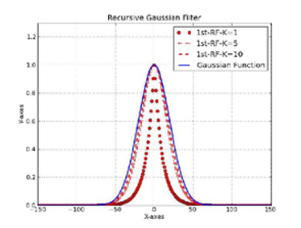
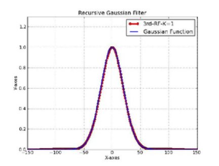
Figure 1: Left - The Impulse response $h_{i}$ (red) resulting from the application of equations (14) and (16) for $K=1,5,10$ and the true gaussian function $g_{i}$ (blue) with non-dimensional length scale $\sigma=R/\delta_{x}$ and mean $\mu=0$
Right - The Impulse response $h_{i}$ (red) resulting from the application of equations (28) and (29) for $K=1$ and the true gaussian function $g_{i}$ (blue) with non-dimensional length scale $\sigma=R/\delta_{x}$ and mean $\mu=0$

About the computational cost of RF we consider the following Remark 2.

• The computational time of a $n-$th order accuracy RF is given by the following formula:

  $$T(n,K,m)\approx 2\ (2n+1)\ m\ K\ t_{calc}.$$ (25)

  where $t_{calc}$ is the time for a floating point operation.

It immediately follows that the time complexity of the 1st-RF is:

$$T(1,K,m)\approx 6mK\ t_{calc}$$ (26)

Unfortunately, the 1st-RF needs a high step number $K$ to determine a good approximation of the convolution function. We underline that this is a huge obstacle in the OceanVar framework since the RF iterations are too much expensive from a computational point of view for real applications. Although the 3rd-RF complexity is

$${T(3,K,m)\approx 14\ mK\ \ t_{calc}}$$ (27)

we have good approximation of the convolution kernel within just one iteration. Note that by comparing the time complexities given by (26) and (27) it follows that the theoretical computational time of the 1st-RF is less than that of the 3rd-RF only if 1 or 2 iterations are used, which however provides a very inaccurate approximation of the Gaussian function.
In the next section, we prove it through numerical experiments, confirming that the new 3rd-RF in OceanVar can improve the entire performance of the data assimilation software.

4 Experimental Results of OceanVar using 1st-RF and 3rd-RF in Mediterranean Sea Implementation

In this section we test the OceanVar set-up in the Mediterranean Sea with both 1st-RF and 3rd-RF from a numerical point of view. Either 1st-RF and 3rd-RF allow to use different filtering scales as we will show in the next section for global applications but in this configuration we fix a constant length scale. This set-up follows the configuration of Dobricic and Pinardi (2008), but the horizontal resolution is two times higher. In particular, the model has 72 horizontal levels, and the horizontal resolution is about 3.5 km in the latitudinal direction and between 3 km and 2.5 km in the longitudinal direction with an horizontal grid of $(1,742,506)$ points. The Mediterranean Sea has a relatively large variability of the bathymetry, with both deep ocean basins, like the Ionian Sea, the Levantine and the Western Mediterranean, and extended narrow shelves.
In this configuration we apply the 1st-RF and the 3rd-RF with the assimilation of only Argo floats profiles (Poulain et al., 2007). We compare accuracy, computational time and the memory usage. The numerical tests are carried out on a parallel IBM cluster (with 30 IBM P575 nodes, 960 cores Power6 4.7GHz, Infiniband 4x DDR interconnection, Operating system AIX v.5.3).

In the following we start to compare the accuracy of horizontal covariances in temperature by means of the two different RFs.
In Figure 2, we report analysis increment obtained using only one iteration of 3rd-RF on the Mediterranean Sea, for the temperature at $300m$, assuming isotropic and Gaussian spatial correlations by means a constant correlation radius ($R=15000m$). The impression in Figure 2 is that the 3rd-RF reconstructs quite successfully the horizontal covariances in just one iteration. The long range correlation shows more a diamond-like shape but the inner part, the most intense part of the field, has the right shape and amplitude. Moreover we underline that the 3rd-RF models the horizontal covariances near the costs using the same number of the imaginary sea points used for the 1st-RF (Dobricic and Pinardi, 2008) because the approximate gaussian functions built by both the RFs have the same length scales.
Then we compute the horizontal temperature covariances at same depth by means of the 1st-RF using K=1 iteration (1st-RF-K=1) in Figure 3a, 1st-RF, K=5 iterations (1st-RF-K=5) in Figure 3b and 1st-RF, K=10 iterations (1st-RF-K=10) in Figure 3c. We can note that only with the 1st-RF K=10 (Figure 3c) the horizontal covariances became isotropic and Gaussian. Figure 4 shows the absolute differences between the horizontal temperature covariances computed by 1st-RF-K=1,5,10 and the 3rd-RF. Observing the maximum values ​​of the differences in the three case, it is evident that the same accuracy of the 3rd-RF can be achieved only with a large number of iterations of the other one . Qualitatively the results for the salinity are the same as for temperature and hence we do not show them.

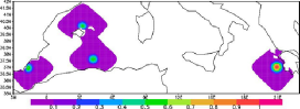
Figure 2: Analysis increments of temperature at 300 m of depth for the Mediterranean Sea configuration using 3rd-RF.

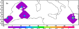
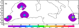
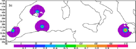
Figure 3: Analysis increments of temperature at 300 m of depth for the Mediterranean Sea configuration using 1st-RF-K=1 (3a), 1st-RF-K=5 (3b) and 1st-RF-K=10 (3c).

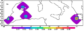
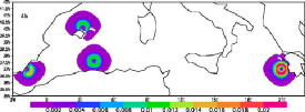
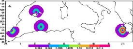
Figure 4: Absolute Differences for the temperature at 300 m of depth for the Mediterranean Sea configuration between 1st-RF-K=1 and 3rd-RF (4a), 1st-RF-K=5 and 3rd-RF (4b), 1st-RF-K=10 and 3rd-RF (4c).

4.1 Performance Results in Mediterranean Sea Implementation

In previous section we show that the use of a more accurate RF needs less iterations in order to obtain isotropic and Gaussian spatial horizontal covariances.
In this subsection we report the benefits and disadvantages of the 3rd-RF from a computational point of view. In particular here we give some information on the execution time and the memory usage in the parallel version of the 1st-RF and 3rd-RF of Oceanvar in Mediterranean Sea configuration.
The parallel implementation of the RF in Oceanvar uses communication strategies based on the pipeline method (e.g., Aoyama and Nakano, 1999), because RF is a typical algorithm with flow dependences, where each iteration has to be strictly executed in a pre-fixed order. OceanVar in Mediterranean Sea configuration implements the pipeline method for the RF by using a column-row-wise block distribution of processors and blocking mpi-send and mpi-receive communication functions to transfer the boundary conditions. All the other operators in OceanVar (vertical EOFs, Vv, barotropic operator, Vn, velocities operator, Vuv, and divergence damping filter, Vd), along with the computations in observation space (misfits update, etc.) follow a Cartesian domain decomposition. The parallel implementation is also completely independent from that of the ocean model used for the forecasts. We modify OceanVar by substituting the 1st-RF with the 3rd-RF, without modifying the pipeline method.
As 3rd-RF needs only one iteration, it requires a smaller number of mpi-communications. This results in a sensible reduction in the latency in the communications. However 3rd-RF has to transfer a larger amount of data in each iteration. For example in the case of 1st-RF, in the forward filtering, the left processor sends only data on its last column to the right processor while in the case of 3rd-RF, the left processor sends data on its last three columns to the right processor.
Figure 5 shows the execution time in seconds and the memory usage in Gbyte of the OceanVar with 1st-RF-K=1, 1st-RF-K=5, 1st-RF-K=10 and 3rd-RF on the IBM cluster using 64 processors. In particular we report the OceanVar and the RF wall clock times. To estimate the RF times in the software we synchronize all the processes in our mpi-communicator by using MPI-Barrier, before and after the implementation of RF.
Figure 5 shows that Oceanvar with the 3rd-RF gives the best results in terms of the execution time if we consider the accuracy on the horizontal covariances discussed in previous section. The 3rd-RF compared to the 1st-RF-K=5 and the 1st-RF-K=10 reduces the wall clock time of the software respectively of about $27\%$ and $48\%$. The execution time is reduced because the new RF decreases the sequential time of each process in the mpi-communicator and needs only one mpi-send and mpi-receive communication for each process. The 3rd-RF algorithm uses twice as much memory than 1st-RF, because it has twice the number of the filter coefficients. However, this did not represent a problem on our cluster because the maximum memory allowed was about 250 Gb.

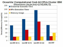
Figure 5: Performance results (execution time and memory usage) for the recursive filter tests within the Mediterranea Sea implementation of OceanVar.

5 Experimental Results of OceanVar using 1st-RF and 3rd-RF in a Global Implementation

In this section we describe experimental results of the 3rd-RF in a Global Ocean implementation of OceanVar that follows Storto et al. (2011). The model resolution is about ${1}/{4}$ degree and the horizontal grid is tripolar, as described by Madec and Imbard (1996). This configuration of the model is used at CMCC for global ocean physical reanalysis applications (Ferry et al., 2012). The model has 50 vertical depth levels. The three-dimensional model grid consists of 73614100 grid-points. The comparison between the 1st-RF and the 3rd-RF is here carried out for a realistic case study, where all in-situ observations of temperature and salinity from Expendable bathythermographs (XBTs), Conductivity, Temperature, Depth (CTDs) Sensors, Argo floats and Tropical mooring arrays are assimilated. The observational profiles are collected, quality-checked and distributed by Coriolis (Cabanes et al., 2013). The global application of the recursive filter accounts for spatially varying and season-dependent correlation length-scales (CLSs), unlike the Mediterranean Sea implementation. Correlation length-scale were calculated by applying the approximation given by Belo Pereira and Berre (2006) to a dataset of monthly anomalies with respect to the monthly climatology, with inter-annual trends removed. The two panels of Figure 6 shows an example of zonal and meridional temperature correlation length-scales at 100 m of depth, respectively, for the winter season in the Western Pacific.

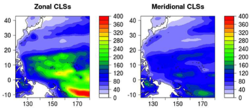
Figure 6: Zonal (left) and meridional (right) correlation length-scales for temperature at 100 m of depth for the Western Pacific Area.

Typically, areas characterized by strong variability (e.g. Kuroshio Extension) present shorter correlation length-scales of the order of less than 100 Km that lead to very narrow corrections, while in the Tropics the length-scales are longer and may reach up to 350 Km, thus broadening the 3DVAR corrections. Furthermore, at the Tropics, it is acknowledged that zonal correlations are longer than the meridional ones (e.g. Derber and Rosati, 1989). The analysis increments from a 3DVAR applications that uses the 1st-RF with 1, 5 and 10 iterations and the 3rd-RF are shown in Figure 7, with a zoom in the same area of Western Pacific Area as in Figure 6, for the temperature at 100 m of depth.

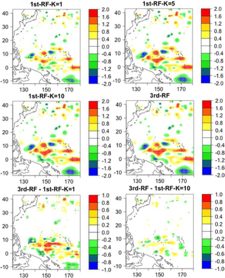
Figure 7: Analysis increments of temperature at 100 m of depth for the Western Pacific for different configurations of the recursive filter (first two rows of panels). Differences of 100 m temperature analysis increments between 3rd-RF and 1st-RF-K=1 and between 3rd-RF and 1st-RF-K=10 (bottom panels).

The figure also displays the differences between the 3rd-RF and the 1st-RF with either 1 or 10 iterations. The patterns of the increments are closely similar, although increments for the case of 1st-RF-K=1 are generally sharper in the case of both short (e.g. off Japan) or long (e.g. off Indonesian region) CLSs. The panels of the differences reveal also that the differences between 3rd-RF and the 1st-RF-K=10 are very small, suggesting once again that the same accuracy of the 3rd-RF can be achieved only with a large number of iterations for the first order recursive filter.

5.1 Performance Results in Global Implementation

In this subsection we present the performance results of the 3rd-RF with respect to the 1st-RF for the Global Ocean case study. OceanVar is run on a parallel IBM cluster, each of the 482 nodes with two eight-core Intel Xeon processors. We use a cluster different from the one previously introduced for the Mediterranean Sea configuration, in an attempt of presenting performance results also in different computing environments. The global ocean implementation of OceanVar has a parallel implementation that differs from the pipeline method previously presented: it exploits hybrid MPI-OpenMP parallelism, where OpenMP acts over the vertical level loops while MPI over the horizontal grid. This strategy has the advantage of limiting the MPI communication when exploiting the same number of cores, with the shortcoming of being not very flexible (due to the limitations of the cores-per-node number of threads for the OpenMP vertical parallelism). We have used 5 nodes for our tests: 5 MPI processes, 16 threads for a total of 80 cores used. Results are summarized in Figure 8, when the number of iterations of the 3DVAR minimizer is fixed to 30, as in realistic applications.

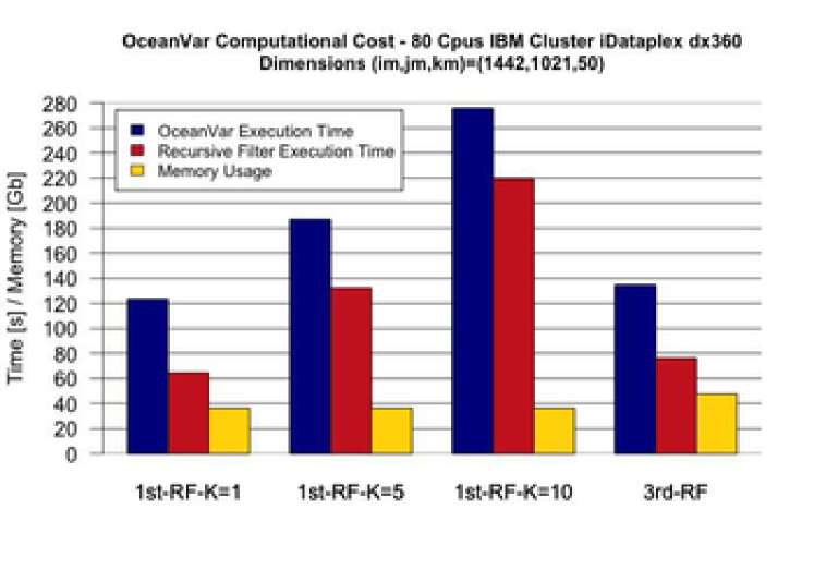
Figure 8: Performance results (execution time and memory usage) for the recursive filter tests within the Global Ocean implementation of OceanVar.

Generally, relative performances of the two recursive filters are comparable with those of the Mediterranean Sea implementation. 3rd-RF reduces the total wall clock time of OceanVar by 28 $\%$ and $51\%$ with respect to 1st-RF-K=5 and 1st-RF-K=10, respectively. This reduction increases up to 42 $\%$ and 65 $\%$ if we consider only the recursive filter routines. On the other hand, the total memory usage increases from 36.4 Gb (7.3 Gb per node) to 47.6 Gb (9.5 Gb per node), i.e. by 30 $\%$. Thus, the third order recursive filter is able to significantly reduce the execution time at the price of an affordable increase of memory usage.

6 Conclusions

In this paper we describe the development and implementation of a revised scheme to compute the horizontal covariances of temperature and salinity in an oceanographic variational scheme.
The existing recursive filter (RF) of the first order (1st-RF) is substituted with a recursive filter of the third order (3rd-RF). Numerical experiments in Mediterranean Sea and Global Ocean demonstrated that a 3rd-RF can significantly reduce the total computational time of the data assimilation scheme maintaining the same level of accuracy.
In addition we provide the full theoretical development of the new filter, based on the study by Young and Van Vliet (1995) and Van Vliet et al. (1998), who formulated the filter in the context of signal processing. We adapt it for a 3D-VAR oceanographic scheme with the detailed description of the process to obtain the 3rd-RF coefficients for different length scales. .
Our implementation is different to that by Purser et al. (2003), since we have applied a different mathematical methodology to calculate the filter coefficients. The new RF is faster than the previous one because it requires only one iteration to compute the horizontal covariances. Therefore, we may assume that it will be faster than other first order accurate methods that need several iterations like the one described by Mirouze and Weaver (2010). This hypothesis is tested with the pipeline method of Mediterranean Sea implementation and hybrid MPI-OpenMPI parallelization strategy of the Global Ocean configuration presented in the previous sections. By applying some other parallelization strategy the relative performance of the new filter may differ. However, we believe that other parallelization strategies are overall much less efficient than those presented.
The future improvement of the 3rd-RF scheme in OceanVar will be the implementation of different mathematical boundary conditions at the coasts and a formulation of 3rd-RF for spatially inhomogeneus and anisotropic covariances.

7 Acknowledgment

The research leading to these results has received funding from the Italian Ministry of Education, University and Research and the Italian Ministry of Environment, Land and Sea under the GEMINA and Next Data projects.

8 Appendix A

• For each $i-th$ grid point of a finite one-dimensional grid with correlation radius $R_{i}$ and grid spacing $\delta x_{i}$, a normalized 3rd-RF is given by:

  $$p_{i}=\beta_{i}s^{0}_{i}+\alpha_{i,1}p_{i-1}+\alpha_{i,2}p_{i-2}+\alpha_{i,3}p_{i-3}\quad i=4,m\ :+1\quad\ \$$ (28)

  $$s_{i}=\beta_{i}p_{i}+\alpha_{i,1}s_{i+1}+\alpha_{i,2}s_{i+2}+\alpha_{i,3}s_{i+3}.\quad i=m-3,1\ :-1.$$ (29)

  where the function $s^{0}_{i}$ is the input distribution, $\alpha_{i,1}=a_{i,1}/a_{i,0}$, $\alpha_{i,2}=a_{i,2}/a_{i,0}$, $\alpha_{i,3}=a_{i,3}/a_{i,0}$ and $\beta_{i}=\sqrt[4]{{2\pi\big{(}{R_{i}}/{\delta x_{i}}\big{)}^{2}}}\big{(}1-\big{(}\alpha_{i,1}+\alpha_{i,2}+\alpha_{i,3})\big{)}$ are the filtering coefficients and:

  $$\begin{array}[]{l}a_{i,0}=3.738128+5.788982\bigg{(}\dfrac{R_{i}}{\delta x_{i}}\bigg{)}+3.382473\bigg{(}\dfrac{R_{i}}{\delta x_{i}}\bigg{)}^{2}+1.000000\bigg{(}\dfrac{R_{i}}{\delta x_{i}}\bigg{)}^{3}\\[5.69054pt] a_{i,1}=5.788982\bigg{(}\dfrac{R_{i}}{\delta x_{i}}\bigg{)}+6.764946\bigg{(}\dfrac{R_{i}}{\delta x_{i}}\bigg{)}^{2}+3.000000\bigg{(}\dfrac{R_{i}}{\delta x_{i}}\bigg{)}^{3}\\[5.69054pt] a_{i,2}=-3.382473\bigg{(}\dfrac{R_{i}}{\delta x_{i}}\bigg{)}^{2}-3.000000\bigg{(}\dfrac{R_{i}}{\delta x_{i}}\bigg{)}^{3}\\[5.69054pt] a_{i,3}=1.000000\bigg{(}\dfrac{R_{i}}{\delta x_{i}}\bigg{)}^{3}\\ \end{array}$$

• In order to obtain an efficient RF such that approximates the gaussian convolution (as considered in Mirouze and Weaver (2010)):

  $$s(x)=g(x)\otimes s^{0}(x)=\int_{-\infty}^{+\infty}g(x-\tau)s^{0}(\tau)d\tau,$$ (30)

  we apply the Fourier transformation to the equation in (30), where $g(x)=\exp(-\frac{x^{2}}{2\sigma^{2}})$ is the normalized gaussian function of mean $\mu=0$ and non-dimensional length-scale $\sigma=R_{i}/\delta x_{i}$ associated to i$-th$ grid point. Hence we obtain:

  $${S(w)}={G(w)}{S^{0}(w)}\quad w\in\mathbb{R}$$ (31)

  where ${S(w)},{G(w)}$ and ${S^{0}(w)}$ in (31) are respectively the Fourier transformations of the function $s(x),g(x)$, and $s^{0}(x)$. For the Fourier transformation of $g(x)$, we have the well-note result:

  $$G(w)=\sqrt{2\pi}\sigma e^{-\frac{(\sigma\omega)^{2}}{2}}.$$ (32)

  Using a rational approximation of the gaussian function in Abramowitz and Stegun (1965):

  $$\frac{1}{\sqrt{2\pi}}e^{-\frac{t^{2}}{2}}=\frac{1}{b_{0}+b_{2}t^{2}+b_{4}t^{4}+b_{6}t^{6}}+\epsilon(t),\quad t\in\mathbb{R}$$ (33)

  where $b_{0}=2.490895$, $b_{2}=1.466003$, $b_{4}=-0.024393$, $b_{6}=0.178257$ and $\epsilon(t)<2.7*10^{-3}$, then we can approximate the $G(w)$ function as:

  $$G(w)\approx H_{\sigma}(w)=\frac{{2\pi}\sigma C^{2}}{b_{0}+b_{2}(\sigma w)^{2}+b_{4}(\sigma w)^{4}+b_{6}(\sigma w)^{6}}$$ (34)

  where $C^{2}$ is a square of a normalization constant that we will choose later. The absolute error $|\epsilon(w)|$ between $G(w)$ and $H_{\sigma}(w)$ is less than ${5.4\pi}\sigma\times 10^{-3}$. Moreover we can rewrite the $H_{\sigma}(\omega)$ as a function in the complex field:

  $$H_{\sigma}(s)=\frac{{2\pi}\sigma C^{2}}{b_{0}-b_{2}(\sigma s)^{2}+b_{4}(\sigma s)^{4}-b_{6}(\sigma s)^{6}},\ \ with\ s=i\omega\in\mathbb{C}$$ (35)

  Through the non linear Newton Formula (e.g., Quarteroni et al., 2007), we determinate two real solution $s=\pm 1.16680481/\sigma$ of the polynomial $b_{0}-b_{2}(\sigma s)^{2}+b_{4}(\sigma s)^{4}-b_{6}(\sigma s)^{6}$. After we divide it for $\big{(}(\sigma s)^{2}-1.6680481^{2}\big{)}$ and obtain a polynomial quotient that is difference between a polynomial of fourth degree and second one. Hence the rational polynomial $H_{\sigma}(s)$ can be decomposed in the following way:

  $$H_{\sigma}(s)=H_{\sigma,b}(s)H_{\sigma,f}(s)$$ (36)

  where

  $$H_{\sigma,f}(s)=\dfrac{\sqrt{(2\pi\sigma)}C}{(1.166805+\sigma s)(3.203730+2.215668\sigma s+({\sigma s})^{2})}$$ (37)

  $$H_{\sigma,b}(s)=\dfrac{\sqrt{(2\pi\sigma)}C}{(1.166805-\sigma s)(3.203730-2.215668\sigma s+({\sigma s})^{2})}.$$ (38)

  Using standard approximations as the backward and forward differences for the $\mathcal{Z}$ transformation (e.g., Oppenheim et al., 1983) to switch from continuous to discrete problem, we replace $s=1-z^{-1}$ in (37) and $s=z-1$ in (38) as in Young and Van Vliet (1995). Hence we obtain:

  $$H_{\sigma,f}(z^{-1})=\dfrac{\sqrt{(2\pi\sigma)}C}{\big{(}1.166805+\sigma(1-z^{-1})\big{)}\big{(}3.203730+2.215668\sigma(1-z^{-1})+({\sigma(1-z^{-1})})^{2}\big{)}}$$

  $$H_{\sigma,b}(z)=\dfrac{\sqrt{(2\pi\sigma)}C}{\big{(}1.166805-\sigma(z-1)\big{)}\big{(}3.203730-2.215668\sigma{(z-1})+({\sigma(z-1)})^{2}\big{)}}$$

Both previous equations can be rewritten respectively as standard polynomials in $z^{-1}$ and $z$:

$$H_{\sigma,f}(z^{-1})=\dfrac{\sqrt{(2\pi\sigma)}C}{\big{(}a_{i,0}-a_{i,1}z^{-1}-a_{i,2}z^{-2}-a_{i,3}z^{-3}\big{)}}\ \$$ (39)

$$H_{\sigma,b}(z)=\dfrac{{\sqrt{(2\pi\sigma)}C}}{\big{(}a_{i,0}-a_{i,1}z^{1}-a_{i,2}z^{2}-a_{i,3}z^{3}\big{)}}\qquad\ \ \ \ .$$ (40)

where we can determinate the following coefficients for (39) and (40):

$$\begin{array}[]{l}a_{i,0}=\big{(}3.738128+5.788982\sigma+3.382472\sigma^{2}+1.000000\sigma^{3})\\[2.84526pt] a_{i,1}=\big{(}5.788824\sigma+6.764946\sigma^{2}+2.999999\sigma^{3})\\[2.84526pt] a_{i,2}=\big{(}-3.382472\sigma^{2}-2.999999\sigma^{3})\\[2.84526pt] a_{i,3}=\big{(}1.000000\sigma^{3})\end{array}$$ (41)

The normalized constant $C$ can be specified by using the constrain that the approximation gaussian function $H_{\sigma}(\omega)$ must be $\sqrt{2\pi}\sigma$ for $\omega=0$ (see the equations (32) and (34)) hence $H_{\sigma,f}(z^{-1})=1\wedge H_{\sigma,b}(z)=\sqrt[4]{(2\pi\sigma^{2})}$ for $z^{-1}=1\wedge z=1$ . Follows that:

$$C=\frac{\big{(}a_{i,0}-(a_{i,1}+a_{i,2}+a_{i,3})\big{)}}{\sqrt[4]{(2\pi)}}$$ (42)

Place $P(z)=H_{\sigma,f}(z)S^{0}(z)$ and $S(z)=H_{\sigma,b}(z)P(z)$, we have:

$$H_{\sigma,f}(z)=\dfrac{P(z)}{S^{0}(z)}=\frac{{\sqrt[4]{(2\pi\sigma^{2})}\big{(}a_{i,0}-(a_{i,1}+a_{i,2}+a_{i,3})\big{)}}}{\big{(}a_{i,0}-a_{i,1}z^{-1}-a_{i,2}z^{-2}-a_{i,3}z^{-3}\big{)}}$$ (43)

$$H_{\sigma,b}(z)=\dfrac{S(z)}{P(z)}=\frac{\sqrt[4]{(2\pi\sigma^{2})}{\big{(}a_{i,0}-(a_{i,1}+a_{i,2}+a_{i,3})\big{)}}}{\big{(}a_{i,0}-a_{i,1}z-a_{i,2}z^{2}-a_{i,3}z^{3}\big{)}}\qquad\ \ \$$ (44)

from which we obtain respectively:

$$\big{(}a_{i,0}-a_{i,1}z^{-1}-a_{i,2}z^{-2}-a_{i,3}z^{-3}\big{)}P(z)=\sqrt[4]{(2\pi\sigma^{2})}\big{(}a_{i,0}-(a_{i,1}+a_{i,2}+a_{i,3})\big{)}S^{0}(z),$$ (45)

$$\big{(}a_{i,0}-a_{i,1}z^{-1}-a_{i,2}z^{-2}-a_{i,3}z^{-3}\big{)}S(z)=\sqrt[4]{(2\pi\sigma^{2})}\big{(}a_{i,0}-(a_{i,1}+a_{i,2}+a_{i,3})\big{)}P(z).\quad$$ (46)

Antitransforming, by means of the $\mathcal{Z}^{-1}$ transformation, the equations (45) and (46) and by the theorem of the delay (e.g., Oppenheim et al., 1983), we obtain the following forward and backward finite difference equations:

$$p_{i}=\beta s^{0}_{i}+\alpha_{i,1}p_{i-1}+\alpha_{i,2}p_{i-2}+\alpha_{i,3}p_{i-3}.$$ (47)

$$s_{i}=\beta p_{i}+\alpha_{i,1}s_{i+1}+\alpha_{i,2}s_{i+2}+\alpha_{i,3}s_{i+3}.\$$ (48)

where the functions $p_{i}$ and $s_{i}$ are respectively the $\mathcal{Z}^{-1}$ transformations of $P(z)$ and $S(z)$ functions and the filtering coefficients are $\alpha_{i,1}=a_{i,1}/a_{i,0}$, $\alpha_{i,2}=a_{i,2}/a_{i,0}$, $\alpha_{i,3}=a_{i,3}/a_{i,0}$ and $\beta_{i}=\sqrt[4]{(2\pi\sigma^{2})}\big{(}1-(\alpha_{i,1}+\alpha_{i,2}+\alpha_{i,3})\big{)}$. Remembering that $\sigma=R_{i}/\delta x_{i}$ and observing the equations (41), (47) and (48) and the values of the filtering coefficients $\alpha_{i,1},\alpha_{i,2},\alpha_{i,3}$ and $\beta_{i}$, then we obtain the thesis. $\blacksquare$

• For an arbitrary input distribution $s^{0}_{i}$, a measure for accuracy of a RF is given by the following inequality:

  $$\|\epsilon_{s_{i}}\|_{2}\leq\|\epsilon_{h_{i}}\|_{2}\|s^{0}_{i}\|_{2}$$ (49)

  where:

  • $\|\epsilon_{s_{i}}\|_{2}$ is the euclidean norm of the difference between the discrete convolution $s^{*}_{i}=g_{i}\otimes s^{0}_{i}$(with $g_{i}$ normalized gaussian function) and the function $s_{i}$, obtained by the RF applied to $s^{0}_{i}$.

  • $\|\epsilon_{h_{i}}\|_{2}$ is the euclidean norm of the difference between the gaussian $g_{i}$ and the function $h_{i}$ (called impulse response), obtained by a RF applied to Dirac function;

  • $\|s^{0}_{i}\|_{2}$ is the euclidean norm of the input function $s^{0}_{i}$ .

• The error in the output per sample when we substitute the true convolution $s^{*}_{i}$ with an approximation $s_{i}$ is given by

  $${\epsilon}_{s_{i}}=s^{*}_{i}-s_{i}=(g_{i}-h_{i})\otimes s^{0}_{i}=\varepsilon_{h_{i}}\otimes s^{0}_{i}.$$ (50)

  Hence it holds the following:

  $$\|\epsilon_{s_{i}}\|_{2}=\|\epsilon_{h_{i}}\otimes s^{0}_{i}\|_{2}$$ (51)

  and applying the Cauchy-Schwarz inequality to the right-hand side of equation (51), it gives the thesis:

  $$\|\epsilon_{s_{i}}\|_{2}\leq\|\epsilon_{h_{i}}\|_{2}\|s_{i}\|_{2}$$ (52)

  $\blacksquare$

References

References

- Abramowitz and Stegun (1965) Abramowitz, M., Stegun, I., 1965. Handbook of Mathematical Functions. Dover, New York.
- Aoyama and Nakano (1999) Aoyama, Y., Nakano, J., 1999. RS/6000 SP: Practical MPI Programming. International Technical Support Organization IBM.
- Belo Pereira and Berre (2006) Belo Pereira, M., Berre, L., 2006. The use of an ensemble approach to study the background-error covariances in a global NWP model . Mon. Wea. Rev. 134, 2466–2489.
- Byrd et al. (1995) Byrd, R., Nocedal, J., Zhu, C., 1995. A limited memory algorithm for bound constrained optimization. SIAM Journal on Scientific Computing 16, 1190–1208.
- Cabanes et al. (2013) Cabanes, C., Grouazel, A., von Schuckmann, K., Hamon, M., Turpin, V., Coatanoan, C., Paris, F., Guinehut, S., Boone, C., Ferry, N., de Boyer Montégut, C., Carval, T., Reverdin, G., Pouliquen, S., Traon, P.-Y. L., 2013. The CORA dataset: validation and diagnostics of in-situ ocean temperature and salinity measurements . Ocean Sci. 9, 1–18.
- Derber and Rosati (1989) Derber, J., Rosati, A., 1989. A global oceanic data assimilation system . J. Phys. Oceanogr. 19, 1333–1347.
- Deriche (1987) Deriche, R., 1987. Separable recursive filtering for efficient multi-scale edge detection . Proc. Internat. Workshop on industrial Application of Machine Vision and Machine Vision and Machine Intelligence, Tokyo, 18–23.
- Dobricic and Pinardi (2008) Dobricic, S., Pinardi, N., 2008. An oceanographic three-dimensional variational data assimilation scheme. Ocean Modeling 22, 89–105.
- Ferry et al. (2012) Ferry, N., Barnier, B., Garric, G., Haines, K., Masina, S., Parent, L., Storto, A., Valdivieso, M., Guinehut, S., Mulet, S., 2012. NEMO: the modeling engine of global ocean reanalyses . Mercator Ocean Quaterly Newsletter 46, 60–66.
- Haben et al. (2011) Haben, S., Lawless, A., Nicholos, N., 2011. Conditioning and preconditioning of the variational data assimilation problem. Computers and Fluids 46, 252–256.
- Hayden and Purser (1995) Hayden, C., Purser, R., 1995. Recursive filter objective analysis of meteorological fields: applications to NESDIS operational processing. Journal of Applied Meteorology 34, 3–15.
- Lorenc (1992) Lorenc, A., 1992. Iterative analysis using covariance functions and filters. Quarterly Jounrnal of the Royal Meteorological Society 1 118, 569–591.
- Madec and Imbard (1996) Madec, G., Imbard, M., 1996. A global ocean mesh to overcome the north pole singularity . Clim. Dynamics 12, 381–388.
- Mirouze and Weaver (2010) Mirouze, I., Weaver, A., 2010. Representation of correlation functions in variational assimilation using an implicit diffusion operator. Quarterly Journal of the Royal Meteorological Society 136, 1421–1443.
- Oppenheim et al. (1983) Oppenheim, A., Willsky, A., Nawab, S., 1983. Signals and Systems. Prentice-Hall.
- Pinardi et al. (2010) Pinardi, N., Allen, I., Demirov, E., Mey, P. D., Korres, G., Lascaratos, A., Traon, P. L., Maillard, C., Manzella, G., Tziavos, C., 2010. The Mediterranean ocean forecasting system: first phase of implementation. Annales Geophysicae 21 21, 3–20.
- Poulain et al. (2007) Poulain, P., Barbanti, R., Font, J., Cruzado, A., Millot, C., Gertman, I., , Griffa, A., Molcard, A., Rupolo, V., Bras, S. L., Petit de la Villeon, L., 2007. MedArgo: a drifting profiler program in the Mediterranean Sea. Ocean Sciences 3, 379–395.
- Purser et al. (2003) Purser, R., Wu, W., Parish, D., Roberts, N., 2003. Numerical aspects of the application of recursive filters to variational statistical analysis. Part I: spatially homogeneous and isotropic covariances. Monthly Weather Review 131, 1524–1535.
- Quarteroni et al. (2007) Quarteroni, A., Sacco, R., Saleri, F., 2007. Numerical Mathematics. Springer.
- Storto et al. (2011) Storto, A., Dobricic, S., Masina, S., Pietro, P. D., 2011. Assimilating along-track altimetric observations through local hydrostatic adjustments in a global ocean reanalysis system . Mon. Wea. Rev. 139, 738–754.
- Van Vliet et al. (1998) Van Vliet, J., Young, I., Verbee, P., 1998. Recursive Gaussian Derivative Filters. Pattern Recognition, 1998. Proceedings. Fourteenth International Conference 1, 509 – 514.
- Vliet et al. (1998) Vliet, L. V., Young, I., Verbeek, P., 1998. Recursive gaussian derivative filters. International Conference on Pattern Recognition, 509–514.
- Weaver et al. (2003) Weaver, A., Vialard, J., Anderson, D., 2003. Three- and four-dimensional variational assimilation with an ocean general circulation model of the tropical Pacific Ocean. Part 1 formulation, internal diagnostics and consistency checks. Monthly Weather Review 131, 1360–1378.
- Young and Van Vliet (1995) Young, L., Van Vliet, I., 1995. Recursive Implementation of the Gaussian Filter. Signal Processing 44, 139–151.