Constituents of magnetic anisotropy and a screening of spin-orbit coupling in solids

Abstract

Using quantum mechanical perturbation theory (PT) we analyze how the energy of perturbation of different orders is renormalized in solids. We test the validity of PT analysis by considering a specific case of spin-orbit coupling as a perturbation. We further compare the relativistic energy and the magnetic anisotropy from the PT approach with direct density functional calculations in FePt, CoPt, FePd, MnAl, MnGa, FeNi, and tetragonally strained FeCo. In addition using decomposition of anisotropy into contributions from individual sites and different spin components we explain the microscopic origin of high anisotropy in FePt and CoPt magnets.

identifier

The magnetocrystalline anisotropy is a central magnetic property for both fundamental and practical reasons.STOHR ; kota ; kosugi It can depend sensitively on many quantities such as dopants or small changes in lattice constant.fe8n While control of this sensitive quantity can be crucial in many applications, e.g. permanent magnetismkirill , magnetoopticsantonov and magnetoresistive random-access memory devicesnature , it is often unclear what mechanisms are responsible for these anisotropy variations, even from a fundamental point of view. It was understood long agoABRA ; yosida that the magnetic anisotropy energy (MAE) $K$ in bulk materials is a result of simultaneous action of spin-orbit coupling (SOC) and crystal field (CF). While in general this statement is still valid, existing microscopic methods do not accurately describe $K$ in the majority of materials. One can calculate MAE using ab-initio electronic structure methods based on density functional theory, however quantitative agreement is often rather poor. In any case such methods are usually not well equipped to resolve it into components that yield an intuitive understanding, to enable its manipulation and control. Sometimes $K$ is analyzed in terms of SOC matrix elements of ${\xi}\mathbf{l{\cdot}s}$, where ${\xi}$ is the SOC constant. However, this perturbation also induces changes in other terms contributing the total energy, which can affect the MAE as well. Below we show how the actual atomic SOC is ’screened’ in crystals and study spin decomposition of SOC and MAE in real world magnets.

Let us write the total Hamiltonian of magnetic electronic system as

$$H=H_{0}+V$$ (1)

where $H_{0}$ is the non-relativistic Hamiltonian (sum of kinetic and potential energies of electrons) and $V=\xi\mathbf{l{\cdot}s}$ is the SOC Hamiltonian. We assume that $\xi$ is small relative to CF and spin splittings. The change in the total energy of the system when SOC is added (below we call it relativistic part of the total energy) can be written as

$$E=\Delta E_{0}+E_{so}$$ (2)

where $E_{so}$ is the matrix element of SOC with full perturbed wavefunction and $\Delta E_{0}$ is the induced energy change of the scalar-relativistic Hamiltonian ( sum of kinetic and potential energies) due to the SOC perturbation.

Using standard quantum mechanical perturbation theory (PT) each quantity $\left|\phi\right\rangle=\sum\left|n\right\rangle,E=\sum E^{\left(n\right)}$ and $E_{so}=\sum V^{\left(n\right)}$ (wave function, total energy and perturbation $V$) can be expressed as a sum over orders $n$: $V^{\left(n\right)}$ is proportional to $\xi^{n+1}$, while $\left|n\right\rangle$ and $E^{\left(n\right)}$ are of order $\xi^{n}$. Here and hereafter we use superscripts in parentheses to denote the order of perturbation term of the corresponding quantity. Corresponding expansions can be introduced for the total MAE and MAE due to SOC term as $K=\sum K^{\left(n\right)}$ and $K_{so}=\sum K_{so}^{\left(n\right)}$.

If $\left|0\right\rangle$ is an eigenvector of unperturbed system ($H_{0}$) then the total perturbation energy can be found as

$$E=\mathop{\displaystyle\sum}_{n}E^{\left(n\right)}=\mathop{\displaystyle\sum}_{n}\left\langle 0\right|V\left|n\right\rangle=\left\langle 0\right|V\left|\phi\right\rangle$$ (3)

(see, for instance, Eq.5.1.37 in ref.10 ). It is now straightforward to show that

$$E_{so}=\left\langle\phi\right|V\left|\phi\right\rangle=\mathop{\displaystyle\sum}\limits_{n}nE^{\left(n\right)}$$ (4)

so the sum of kinetic and potential energies change can be presented as

$$\Delta E_{0}=\mathop{\displaystyle\sum}\limits_{n}\left(1-n\right)E^{\left(n\right)}=\left(\left\langle 0\right|-\left\langle\phi\right|\right)V\left|\phi\right\rangle$$ (5)

The last expression can be directly evaluated to estimate a reaction of the system to the original perturbation $V$. In our case this reaction corresponds to joint action of kinetic and potential energy terms ($H_{0}$ in Eq.1). Eq.4 is particularly convenient for the analysis due to opportunity to obtain site and spin decompositions.

Let us consider again a specific case of SOC perturbation $V=\xi\mathbf{l{\cdot}s}$ in the second order of PT. In this case we have $E^{\left(2\right)}=E_{so}^{\left(1\right)}/2=V^{\left(1\right)}/2,$ where $V^{\left(1\right)}$ is obtained using wave function of the first order $\left|\phi\right\rangle\approx$ $\left(\left|0\right\rangle+\left|1\right\rangle\right)$. Correspondingly, for the second order MAE

$$K^{(2)}=K_{so}^{\left(1\right)}/2$$ (6)

The second order correction to the total MAE due to SOC is a half of the first order MAE due to SOC only. It is a simple consequence of our perturbation treatment. One can immediately write down the MAE in cubic systems where the leading term scales as $\xi^{4}$, as $K^{(4)}=K_{so}^{\left(3\right)}/4$. Thus kinetic and potential terms effectively ’screen’ 75% of the original SOC MAE in cubic materials. Evidently higher order contributions to total MAE decrease as $1/n$ relative to SOC anisotropy. Thus the highest anisotropy can be naturally expected only for a small $n$.

The specific form of the second order correction due to SOC has been studied many times in different parts of solid state physicsSTOHR ; ABRA ; yosida ; LAAN and can be obtained if we rewrite $V^{\left(1\right)}$ as

$$V^{\left(1\right)} = 2\left\langle 0\right|\xi\mathbf{l{\cdot}s}\left|1\right\rangle=2\xi s_{i}^{\left(0\right)}l_{i}^{\left(1\right)}=$$

$$2\xi s_{i}^{\left(0\right)}\sum_{{exc}}\frac{\left\langle 0\right|l_{i}\left|1\right\rangle\left\langle 1\right|\xi s_{j}l_{j}\left|0\right\rangle}{\varepsilon^{\prime}-\varepsilon_{0}}$$

$$= 2\xi^{2}s_{i}^{\left(0\right)}\sum_{exc}\frac{\left\langle 0\right|l_{i}\left|1\right\rangle\left\langle 1\right|l_{j}\left|0\right\rangle}{\varepsilon^{\prime}-\varepsilon_{0}}s_{j}^{\left(0\right)}$$

$$= 2\xi s_{i}^{\left(0\right)}\Lambda_{ij}s_{j}^{\left(0\right)}$$

where we indicated the specific orders for spin and orbital moments entering $V^{\left(1\right)}$, $\varepsilon_{0}$ and $\varepsilon^{\prime}$ are ground state and excited state energy respectively for the unperturbed system, and the sum is over all excited states. The leading relativistic correction for the spin moment $s$ appears only in the second order in $\xi$ and does not contribute to $V^{\left(1\right)}$. Below we assume that $s$ does not change from its zero order value. This result (Eq.Constituents of magnetic anisotropy and a screening of spin-orbit coupling in solids) is the familiar expression ABRA ; yosida ; LAAN ; STOHR for the second order spin Hamiltonian due to SOC, where orbital moment tensor $\Lambda=$ $l^{\left(1\right)}/\xi s$ . Correspondingly, in the uniaxial system (assuming $\Lambda_{\nu\mu}$ is diagonal) we have $K^{(2)}=\xi s\left(l_{z}^{\left(1\right)}-l_{x}^{\left(1\right)}\right)=\xi^{2}s^{2}(\Lambda_{\perp}-\Lambda_{\parallel}).$

One can regard the total relativistic energy as the energy change due to the “atomic” SOC (i.e. matrix elements of ${\xi}\mathbf{l{\cdot}s}$), ‘screened’ or reduced by adjustments in other contributions to the total energy. The same evidently holds true for the total relativistic energy change relative to SOC energy alone even in the nonmagnetic case. One can rewrite Eq.2 as

$$E=\Delta E_{0}+\left\langle\xi\mathbf{l{\cdot}s}\right\rangle=\langle\widetilde{\xi}\mathbf{l{\cdot}s}\rangle$$ (8)

where $\widetilde{\xi}$ is a screened or effective crystal SOC constant as opposed to the atomic or nonrenormalized $\xi$. We call $\widetilde{\xi}/\xi$ ratio spin-orbit reduction factor. One can compare this parameter with the enhancement of SOC discussed in Ref. yafet, .

According to above results (Eq.4) $\widetilde{\xi}=\xi/2$ (second order correction) and $\widetilde{\xi}=\xi/4$ (fourth order correction). Thus the effective screening is minimal for systems with large SOC and non-cubic symmetries. Evidently this conclusion supports traditionally large anisotropies observed in magnetic uniaxial systems.

Thus $H_{0}$ term in Eq.1, the sum of kinetic and potential energies, reduces the effect of SOC and makes overall strength twice smaller in second order, so $K_{kin}{+}K_{pot}{=}-K_{so}/2$. Overall the action of these terms is destructive for materials with observed uniaxial anisotropy as total $K$ is opposite in sign to the anisotropy induced by kinetic and potential terms together $K=-\left(K_{kin}{+}K_{pot}\right)$. Also comparing Eq.4 and Eq.5 one can see that for arbitrary $n$ ratio $E_{so}^{\left(n\right)}/E_{0}^{\left(n\right)}=n/\left(1-n\right)$, thus for large $n$ this ratio tends to be equal to $-1$ meaning that SOC effects are nearly completely screened in this limit.

Table 1: $c/a$ ratio( with respect to the primitive cell), calculated $K$ and $K_{so}$/$K$ ratio in uniaxial magnetic systems. For all systems experimental structures have been used, while for FeCo , we used hypothetical tetragonally strained structure.

Compounds	$c/a$	$K$($\mu eV$/f.u.)	$K_{so}$/$K$
FePt	1.362	2661	1.84
CoPt	1.379	837	1.67
FeNi	1.414	87	1.98
FePd	1.370	174	2.14
MnAl	1.294	287	1.98
MnGa	1.280	437	1.99
FeCo	1.1	216	2.21

Let us now consider electronic structure calculations for realistic systems. Using the Vienna ab initio simulation packagevasp method we obtained the relativistic energy $E=(E_{r}-E_{nr})$ and SOC energy $E_{so}$ in non-magnetic and magnetic systems, where $E_{nr}$ and $E_{r}$ are total energies obtained in scalar relativistic and calculations where SOC has been added (relativistic). The SOC is included anderson using the second-variation procedure. The generalized gradient approximation of Perdew, Burke, and Ernzerhof was used for the correlation and exchange potentials. The nuclei and core electrons were described by projector augmented wave potentials and the wave functions of valence electrons were expanded in a plane-wave basis set with a energy cutoff between 348 eV and 368 eV for all compounds we investigated in this work. The $k$-point integration was performed using a tetrahedron method with Blöchl corrections with 13800 $k$-points in the first Brillouin zone corresponding to the primitive unit cell of $L1_{0}$ structure.

We compared the spin-orbit reduction factor $\alpha{=}E_{so}/E$ for Al and non-magnetic Fe. The resulting $\alpha$ appears to be very close to 2 with small deviations of about 1-3$\%$. For magnetic systems, we also found that $\alpha{\approx}2$ for different magnetization directions.

MAE in $L1_{0}$ compounds and tetragonal FeCo had been well studiedkota ; kosugi ; ravindran ; solovyev; sakuma; burkert. The calculated MAE values are in reasonable agreement with previous calculationskota ; kosugi . For CoPt, the discrepancy between current calculation and previous ones is rather large. This is due to the exchange correlation potential used, our LDA calculation gives a MAE about 1.3$meV$/f.u., which is in better agreement with previous calculations.

Here we investigated $K_{so}/K$ in those systems and the results are presented in Table 1. The anisotropic part of $E_{so}$ appears to be much smaller than the isotropic part, and deviations of $K_{so}$/$K$ from 2 are already significant. For instance $K_{so}$/ $K$ in CoPt is 1.67-1.8 depending on the exchange-correlation potential used. Compared with $E_{so}$, $K_{so}$ is a much smaller quantity. The deviations of $K_{so}$/$K$ from the factor two in table 1 are related to a deviation from a second order PT. That includes both self-consistency effects and a contribution from higher order terms of PT.

Table 2: Spin decomposition of atomic spin-orbit coupling energy $E_{so}$ (meV) and orbital magnetic moment $M_{l}$ ($10^{-3}\mu_{B}$). $\uparrow\uparrow$ indicates the majority spin channel, and $\downarrow\downarrow$ indicates the minority spin channel. Anisotropies of $E_{so}$ and $M_{l}$ are defined as $K_{so}$=$(E_{so}^{x}-E_{so}^{z})$ and $K_{l}$=$(M_{l}^{z}-M_{l}^{x})$ respectively.

FePt		Pt					Fe
		$\uparrow\uparrow$	$\uparrow\downarrow$	$\downarrow\uparrow$	$\downarrow\downarrow$	Total	$\uparrow\uparrow$	$\uparrow\downarrow$	$\downarrow\uparrow$	$\downarrow\downarrow$	Total
	$z$	-133.80	-281.85	-281.85	-145.66	-843.2	-1.08	-2.47	-2.47	-2.62	-8.6
$E_{so}$	$x$	-125.88	-282.87	-282.87	-145.22	-836.9	-1.53	-2.86	-2.86	-2.83	-10.1
	$K_{so}$	7.92	-1.02	-1.02	0.44	6.3	-0.45	-0.38	-0.38	-0.21	-1.5
	$z$	-113			166	53	-13			77	64
$M_{l}$	$x$	-98			165	67	-23			85	62
	$K_{l}$	-15			1	-14	10			-8	2
CoPt		Pt					Co
		$\uparrow\uparrow$	$\uparrow\downarrow$	$\downarrow\uparrow$	$\downarrow\downarrow$	Total	$\uparrow\uparrow$	$\uparrow\downarrow$	$\downarrow\uparrow$	$\downarrow\downarrow$	Total
	$z$	-134.46	-287.69	-287.69	-151.16	-861.0	-1.40	-2.97	-2.97	-4.97	-12.3
$E_{so}$	$x$	-126.18	-290.64	-290.64	-151.30	-858.8	-1.94	-3.57	-3.57	-4.08	-13.2
	$K_{so}$	8.28	-2.95	-2.95	-0.14	2.2	-0.55	-0.60	-0.60	0.90	-0.90
	$z$	-112			185	72	-16			116	100
$M_{l}$	$x$	-96			188	91	-26			92	66
	$K_{l}$	-16			-3	-19	10			24	34

It had often been discussedSTOHR ; yosida ; streever how a minimum of energy is related to a maximum of orbital magnetic moment $M_{l}$. However, in realistic systems such a relation is often not fulfilled. For example, FePt and CoPt have smaller orbital magnetic moments along the easy axissakuma. In order to understand these phenomena, we resolve SOC energies and orbital moments into atomic and spin contributions for FePt and CoPt (Table 2). $M_{l}$ contains two spin longitudinal contributions $M_{l}=-L_{z}^{\uparrow\uparrow}+L_{z}^{\downarrow\downarrow}$, while the energy $E_{so}^{\left(1\right)}$${\sim}-\xi/2\left(L_{z}^{\uparrow\uparrow}+L_{z}^{\downarrow\downarrow}+L_{-}^{\uparrow\downarrow}+L_{+}^{\downarrow\uparrow}\right)$ also contains spin transversal terms. As shown in Table 2, Pt atoms produce the dominant contribution to $K_{so}$, while Fe (Co) atoms have much smaller and negative values. For each spin component on Pt atom a direct proportionality between the orbital moment and the SOC energy is confirmed, thus a larger component of orbital moment corresponds to the minimum of corresponding energy component. However, this is no longer true for the total moment due to the fact that term with $L_{z}^{\downarrow\downarrow}$ enters definition of total moment and energy with different sign (see above). In addition, as shown in Table 2, while $\downarrow\downarrow$ components of $M_{l}$ and $E_{so}$ are large but rather isotropic, their $\uparrow\uparrow$ components are smaller but much more anisotropic, providing a dominant contribution to the total MAE.

A different behavior of anisotropies of these two spin channels on Pt sites we attribute to the peculiar features in the density of states (DOS). Fig.1 (top) shows the partial DOS projected on the $5d$ states of Pt atom in FePt and CoPt. For the majority spin channel, there are large DOS of all $5d$ states right below the Fermi level and also a large density of state of $d_{x^{2}-y^{2}}$ right at the Fermi level, which is unexpected for elements with nearly filled $d$-band. The minority spin channels have smaller DOS right below the Fermi level, especially for the $d_{x^{2}-y^{2}}$ and degenerated $d_{yz}|d_{xz}$ states. Fig.1 (bottom) shows the schematic representation of difference between FePt DOS and an ideal nearly-filled $d$-band DOS with a large spin-splitting. Hence we would expect the minority spin channel has smaller contribution to MAE than the majority one.

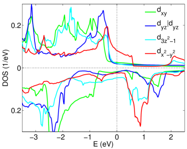
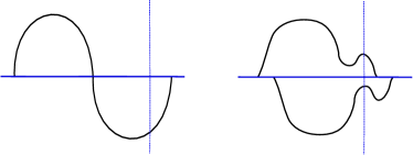
Figure 1: (Color online) Partial density of state (top) projected on the $5d$ states of Pt atom in FePt and schematic (bottom) representation of DOS of an ideal nearly-filled $d$-band and FePt. The vertical dotted line corresponds to the Fermi energy, $E_{F}$.

In this paper using general perturbation theory we discuss how the spin-orbit interaction is renormalized in solids. We show that kinetic and potential energy terms nearly completely ’screen’ spin-orbit coupling at higher orders of perturbation theory. By decomposing the MAE and atomic orbital moments into the sum over different spin matrix elements, we explained why FePt and CoPt have smaller orbital magnetic moments along the easy axis and a microscopic source of large anisotropy in these materials. Such analysis of the SOC energy makes it easier to study atomic decomposition of MAE and other anisotropic effects.

This research is supported in part by the Critical Materials Institute, an Energy Innovation Hub funded by the U.S. Department of Energy, Office of Energy Efficiency and Renewable Energy, Advanced Manufacturing Office and by its Vehicle Technologies Program, through the Ames Laboratory. LLNL is operated under Contract DE-AC52-07NA27344 and Ames Laboratory is operated by Iowa State University under contract DE-AC02-07CH11358.

References

- (1) J. Stöhr and H.C. Siegmann. Magnetism. From fundamentals to Nanoscale Dynamics. Springer-Verlag, Berlin Heidelberg, 2006.
- (2) Y. Kota and A. Sakuma J. Phys. Soc. Jap. 83 034715 (2014 )
- (3) A. Sakuma J. Phys. Soc. Jap. 63 (1994 ) 3053
- (4) L. Ke , K. D. Belashchenko , M. van Schilfgaarde , T. Kotani and V. P. Antropov, Phys. Rev. B 88, 024404 (2013)
- (5) K. D. Belashchenko and V. P. Antropov Phys. Rev. B 66, 144402 (2002)
- (6) V. N. Antonov , V. P. Antropov , B. N. Harmon , A. N. Yaresko and A. Ya. Perlov Phys. Rev. B 59, 14552 (1999)
- (7) J. Hu , Z. Li , L. Chen and C. Nan Nat. Commun. 2 553 (2011 )
- (8) A. Abragam and B. Bleaney, Electron Paramagnetic Resonance of Transition Ions. Oxford University Press, Oxford, 1970.
- (9) K. Yosida, A. Okiji and S. Chikazumi Prog. Theor. Phys. 33 559 (1965)
- (10) J. J. Sakurai, Modern Quantum mechanics. Addison-Wesley Publishing Company, Inc., 1994.
- (11) G. van der Laan. J. Phys.: Condens. Matter 10 3239 (1998)
- (12) Y. Yafet J. Appl. Phys. 39 853 (1968)
- (13) G. Kresse and J. Hafner, Phys. Rev. B 47, 558 (1993); G. Kresse and J. Furthmüller, Phys. Rev. B54, 11 169 (1996); http://cms.mpi.univie.ac.at/vasp.
- (14) O. K. Andersen, Phys. Rev. B 12, 3060 (1975).
- (15) P. Ravindran, A. Kjekshus, H. Fjellv ̵̊ P. James, L. Nordströ˝̈m, B. Johansson, and O. Eriksson, Phys. Rev. B 63, 144409 (2001). \@@lbibitem{solovyev}\NAT@@wrout{16}{}{}{}{(16)}{solovyev}\lx@bibnewblock I. V. Solovyev, P. H. Dederichs, and I. Mertig, Phys. Rev. B 52, 13419 (1995). \@@lbibitem{sakuma}\NAT@@wrout{17}{}{}{}{(17)}{sakuma}\lx@bibnewblock Y. Kota and A. Sakuma J. Phys. Soc. Jap. 81 084705 (2012 ) \@@lbibitem{burkert}\NAT@@wrout{18}{}{}{}{(18)}{burkert}\lx@bibnewblock T. Burkert, L. Nordströ˝̈m, O. Eriksson, and O. Heinonen, Phys. Rev. Lett. 93, 027203 (2004) \@@lbibitem{streever}\NAT@@wrout{19}{}{}{}{(19)}{streever}\lx@bibnewblock R. L. Streever, Phys. Rev. B 19, 2704 (1979) \endthebibliography \par\@add@PDF@RDFa@triples\par\end{document}