Dynamic and Multi-functional Labeling Schemes

Abstract

We investigate labeling schemes supporting adjacency, ancestry, sibling, and connectivity queries in forests. In the course of more than 20 years, the existence of $\log n+O(\log\log)$ labeling schemes supporting each of these functions was proven, with the most recent being ancestry [Fraigniaud and Korman, STOC ’10]. Several multi-functional labeling schemes also enjoy lower or upper bounds of $\log n+\Omega(\log\log n)$ or $\log n+O(\log\log n)$ respectively. Notably an upper bound of $\log n+5\log\log n$ for adjacency+siblings and a lower bound of $\log n+\log\log n$ for each of the functions siblings, ancestry, and connectivity [Alstrup et al., SODA ’03]. We improve the constants hidden in the $O$-notation. In particular we show a $\log n+2\log\log n$ lower bound for connectivity+ancestry and connectivity+siblings, as well as an upper bound of $\log n+3\log\log n+O(\log\log\log n)$ for connectivity+adjacency+siblings by altering existing methods.

In the context of dynamic labeling schemes it is known that ancestry requires $\Omega(n)$ bits [Cohen, et al. PODS ’02]. In contrast, we show upper and lower bounds on the label size for adjacency, siblings, and connectivity of $2\log n$ bits, and $3\log n$ to support all three functions. There exist efficient adjacency labeling schemes for planar, bounded treewidth, bounded arboricity and interval graphs. In a dynamic setting, we show a lower bound of $\Omega(n)$ for each of those families.

1 Introduction

A labeling scheme is a method of distributing the information about the structure of a graph among its vertices by assigning short labels, such that a selected function on pairs of vertices can be computed using only their labels. The concept was introduced in a restricted manner by Bruer and Folkman [1], revisited by Kannan, Naor and Rudich [2], and explored by a wealth of subsequent work [3, 4, 5, 6, 7, 8].

Labeling schemes for trees have been studied extensively in the literature due to their practical applications in improving the performance of XML search engines. Indeed, XML documents can be viewed as labeled forests, and typical queries over the documents amount to testing classic properties such as adjacency, ancestry, siblings and connectivity between such labeled tree nodes [9]. In their seminal paper, Kannan et. al. [2] introduced labeling schemes using at most $2\log n$ bits for each of the functions adjacency, siblings and ancestry. Improving these results have been motivated heavily by the fact that a small improvement of the label size may contribute significantly to the performance of XML search engines. Alstrup, Bille and Rauhe [4] established a lower bound of $\log n+\log\log n$ for the functions siblings, connectivity and ancestry along with a matching upper bound for the first two. For adjacency, a $\log n+O(\log^{*}n)$ labeling scheme was presented in [3]. A $\log n+O(\log\log n)$ labeling scheme for ancestry was established only recently by Fraigniaud and Korman [5].

In most settings, it is the case that the structure of the graph to be labeled is not known in advance. In contrast to the static setting described above, a dynamic labeling scheme typically receives the tree as an online sequence of topological events, with a natural extension that includes removal of leaves. Cohen, Kaplan and Milo [11] considered dynamic labeling schemes where the encoder receives $n$ leaf insertions and assigns unique labels that must remain unchanged throughout the labeling process. In this context, they showed a tight bound of $\Theta(n)$ bits for any dynamic ancestry labeling scheme. We stress the importance of their lower bound by showing that it extends to routing, NCA, and distance as well. In light of this lower bound, Korman, Peleg and Rodeh [13] introduced dynamic labeling schemes, where node re-label is permitted and performed by message passing. In this model they obtain a compact labeling scheme for ancestry, while keeping the number of messages small. Additional results in this setting include conversion methods for static labeling schemes [13, 14], as well as specialized distance [14, 15] and routing [16, 17] labeling schemes. See [18] for experimental evaluation.

Considering the static setting, a natural question is to determine the label size required to support some, or all, of the functions. Simply concatenating the labels mentioned yield a $O(\log n)$ label size, which is clearly undesired. Labeling schemes supporting multiple functions (or multi-functional labeling schemes) were previously studied in [4], showing an upper bound of $\log n+5\log\log n$ bits for combined adjacency and sibling queries. We observe, that their scheme can be combined with the ideas of [3] to produce a $\log+2\log\log n$ labeling scheme for adjacency and siblings.

See Table 1 for a summary of labeling schemes for forests including the results of this paper.

Function	Static Label Size	Static Lower Bound	Dynamic
Adjacency	$\log n+O(\log^{*}n)$ [3]	$\log n+O(1)$	$2\log n$ (Th. 3.1)
Connectivity	$\log n+\log\log n$ [4]	$\log n+\log\log n$ [4]	$2\log n$ (Th. 3.1)
Sibling	$\log n+\log\log n$ [10]	$\log n+\log\log n$ [4]	$2\log n$ (Th. 3.1)
Ancestry	$\log n+4\log\log n$ [5]	$\log n+\log\log n$ [4]	$n$ [11]
AD/S	$\log n+2\log\log n$ (Cor. 2)	$\log n+\log\log n$ [4]	$2\log n$ (Th. 3.1)
C/S	$\log n+2\log\log n$ (Th. 4.2)	$\log n+2\log\log n$ (Th. 4.4)	$3\log n$ (Th. 4.1)
C/AN	$\log n+5\log\log n$ (Th. 4.2)	$\log n+2\log\log n$ (Th. 4.5)	$n$ [11]
C/AD/S	$\log n+3\log\log n$ (Cor. 2)	$\log n+2\log\log n$ (Th. 4.4)	$3\log n$ (Th. 4.1)
Routing	$(1+o(1))\log n$ [7]	$\log n+\log\log n$ [4]	$n$ (Sec. 3)
NCA	$2.772\log n$ [6]	$1.008\log n$ [6]	$n$ (Sec. 3)
Distance	$1/2\log^{2}n$ [8]	$1/8\log^{2}n$ [8]	$n$ (Sec. 3)
Sibling*	$\log n$	$\log n$	$\log n$
Connectivity*	$\log n$	$\log n$	$\log n$
C/S*	$\log n+\log\log n$ (Th. 4.2)	$\log n+\log\log n$ (Th. 4.3)	$2\log n$

Table 1: Upper and lower label sizes for labeling trees with $n$ nodes (excluding additive constants). Routing is reported in the designer-port model [12] and NCA with no pre-existing labels [6], functions marked with * denote non-unique labeling schemes, and bounds without a reference are folklore. Dynamic labeling schemes are all tight.

1.1 Our contribution

We first observe that for the dynamic setting, we can achieve efficient labeling schemes for the functions adjacency, sibling, and connectivity without the need of relabeling. More precisely, we observe that the original $2\log n$ adjacency labeling scheme due to Kannan et. al. [2] is in fact suitable for the dynamic setting. Moreover, the original labeling scheme also supports sibling queries and a slightly modified scheme is shown to work for connectivity. We also present simple families of insertion sequences for which labels of size $2\log n$ are required, showing that in the dynamic setting the original labeling schemes are in fact optimal. The result is in contrast to the static case, where adjacency labels requires strictly fewer bits than both sibling and connectivity. The labeling schemes also reveal an exponential gap between ancestry and the functions mentioned for the dynamic setting. In Section 3.3 we show a construction of simple lower bounds of $\Omega(n)$ for adjacency labeling schemes on various important graph families.

In the context of multi-functional labeling schemes, we show the following results. First, we show that $3\log n$ bits are necessary and sufficient for any dynamic labeling scheme supporting adjacency and connectivity. Turning to static labeling schemes, we show a tight $\log n+2\log\log n$ bound for any unique labeling scheme supporting both connectivity and siblings/ancestry. For the upper bound, we prove the more general result, that any labeling scheme of size $S(n)$ growing faster than $\log n$ can be altered to support connectivity as well by adding at most $\log\log n$ bits. Coupled with our observation, that [3] and [4] provide a $\log n+2\log\log n$ scheme for adjacency and sibling, this provides a $\log n+3\log\log n$ labeling scheme for all the functions adjacency, sibling and connectivity.

2 Preliminaries

A binary string $x$ is a member of the set $\{0,1\}^{*}$, and we denote its size by $|x|$, and the concatenation of two binary strings $x,y$ by $x\circ y$.

A label assignment for a tree $T$ is a mapping of each $v\in V$ to a bit string $\mathcal{L}(v)$, called the label of $v$. Given a tree $T=(V,E)$ rooted in $r$ with $n$ nodes, and let $u,v\in V$. The function $adjacency(v,u)$ returns true if and only if $u$ and $v$ are adjacent in $T$, $ancestry(v,u)$ returns true if and only if $u$ is on the path $r\leadsto v$, $siblings(v,u)$ returns true if and only if $u$ and $v$ have the same parent in $T$, $routing(v,u)$ returns an identifier of the edge connected to $u$ on the path to $v$, $NCA(v,u)$ returns the label of the first node in common on the paths $u\leadsto r$ and $v\leadsto r$, and $distance(v,u)$ returns the length of the path from $v$ to $u$. The functions mentioned previously are also defined for forests. Given a rooted forest $F$ with $n$ nodes, for any two nodes $u,v$ in $F$ the function $connectivity(v,u)$ returns true if $v$ and $u$ are in the same tree in $F$.

Given a function $f$ defined on sets of vertices, an f-labeling scheme for a family of graphs $\mathcal{G}$ consists of an encoder and decoder. The encoder is an algorithm that receives a graph $G\in\mathcal{G}$ as input and computes a label assignment $e_{G}$. If the encoder receives $G$ as a sequence of topological events the labeling scheme is dynamic. The decoder is an algorithm that receives any two labels $\mathcal{L}(v),\mathcal{L}(u)$ and computes the query $d(\mathcal{L}(v),\mathcal{L}(u))$, such that $d(\mathcal{L}(v),\mathcal{L}(u))=f(v,u)$. The size of the labeling scheme is the maximum label size. If for all graphs $G\in\mathcal{G}$, the label assignment $e_{G}$ is an injective mapping, i.e. for all distinct $u,v\in V(G)$, $e_{G}(u)\neq e_{G}(v)$, we say that the labeling scheme assigns unique labels. Unless stated otherwise, the labeling schemes presented are assumed to assign unique labels. Moreover, we allow the decoder to know the label size.

Let $H$ be a family of graphs, a graph $G\in H$, and suppose that an f-labeling scheme assigns a node $v\in G$ the label $\mathcal{L}(v)$. If $\mathcal{L}(v)$ does not appear in any of the label assignments for the other graphs in $H$, we say that the label is distinct for the labeling scheme over $H$. All labeling schemes constructed in this paper require $O(n)$ encoding time and $O(1)$ decoding time under the assumption of a $\Omega(n)$ word size RAM model. See [7] for additional details.

3 Dynamic labeling schemes

We first note that the lower bound for ancestry due to Cohen, et. al. also holds for NCA, since the labels computed by an NCA labeling scheme can decide ancestry: Given the labels $\mathcal{L}(u),\mathcal{L}(v)$ of two nodes $u,v$ in the tree $T$, return true if $\mathcal{L}(u)$ is equal to the label returned by the original NCA decoder, and false otherwise. Similarly, suppose a labeling scheme for routing assigns $0$ as the port number on the path to the root. Given $\mathcal{L}(u),\mathcal{L}(v)$ as before, return true if $routing(\mathcal{L}(u),\mathcal{L}(v))\neq 0$ and $routing(\mathcal{L}(v),\mathcal{L}(u))=0$. Peleg [19] proved that any $f(n)$ distance labeling scheme can be converted to $f(n)+\log(n)$ labeling scheme for NCA by attaching the depth of any node. Since the depth of a node inserted can not change in our dynamic setting, we conclude that any lower bound for ancestry also applies to distance, routing, and NCA.

3.1 Upper Bounds

The following (static) adjacency labeling scheme was introduced by Kannan et al. [2]. Consider an arbitrary rooted tree $T$ with $n$ nodes. Enumerate the nodes in the tree with the numbers $0$ through $n-1$, and let, for each node $v$, $Id(v)$ be the number associated with $v$. Let $parent(v)$ be the parent of a node $v$ in the tree. The label of $v$ is $\mathcal{L}(v)=(Id(v),Id(parent(v)))$, and the root is labeled $(0,0)$. Given the labels $\mathcal{L}(v),\mathcal{L}(v^{\prime})$ of two nodes $v$ and $v^{\prime}$, observe that the two nodes are adjacent if and only if either $Id(parent(v))=Id(v^{\prime})$ or $Id(parent(v^{\prime}))=Id(v)$ but not both, so that the root is not adjacent to itself.

This is also a dynamic labeling scheme for adjacency with equal label size. Moreover, it is also both a static and dynamic labeling scheme for sibling, in which case, the decoder must check if $Id(parent(v))=Id(parent(v^{\prime}))$. A labeling scheme for connectivity can be constructed by storing the component number rather than the parent id. After $n$ insertions, each label contains two parts, each in the range $[0,n-1]$. Therefore, the label size required is $2\log n$.

The labeling schemes suggested extend to larger families of graphs. In particular, the dynamic connectivity labeling scheme holds for the family of all graphs. The family of $k$-bounded degree graphs enjoys a similar dynamic adjacency labeling scheme of size $(k+1)\log n$.

3.2 Lower Bounds

We show that $2\log n$ is in fact a tight bound for any dynamic adjacency labeling scheme for trees. We denote by $\mathcal{F}_{n}(k)$ an insertion sequence of $n$ nodes, creating an initial path of length $1<k\leq n$, followed by $n-k$ adjacent leaves to node $k-1$ on the path. The family of all such insertions sequences is denoted $\mathcal{F}_{n}$. For illustration see Fig. 1.

Lemma 1.

Fix some dynamic labeling scheme that supports adjacency. For any $1<k<n$, $\mathcal{F}_{n}(k)$ must contain at least $n-k$ distinct labels for this labeling scheme over $\mathcal{F}_{n}$.

Proof.

The labels of $\mathcal{F}_{n}(n)$ are set to $P_{1}\dots P_{n}$ respectively. Since the encoder is deterministic, and since every insertion sequence $\mathcal{F}_{n}(k)$ first inserts nodes on the initial path,these nodes must be labeled $P_{1}\dots P_{k}$. Let the labels of the adjacent leaves of such an insertion sequence be denoted by $L^{k}_{1}\dots L^{k}_{n-k}$.

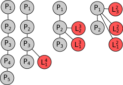
Figure 1: Illustration of $\mathcal{F}_{5}$.

Clearly, $L_{1}^{k}\dots L_{n-k}^{k}$ must be different from $P_{1}\dots P_{n}$, as the only other labels adjacent to $P_{k-1}$ are $P_{k-2}$ and $P_{k}$, which have already been used on the initial path. Consider now any node labeled $L_{i}^{j}$ of $\mathcal{F}_{n}(j)$ for $j\neq k$. Assume w.l.o.g that $j>k$. Such a node must be adjacent to $P_{j-1}$ and not to $P_{k-1}$, as $P_{k-1}$ is contained in the path to $P_{j-1}$. Therefore we must have $L_{i}^{j}\notin\{L_{1}^{k},\dots,L_{n-k}^{k}\}$. ∎

Identical lower bounds exist for both sibling and connectivity, see App. 0.A.1.

Theorem 3.1.

Any dynamic labeling scheme supporting either adjacency, connectivity, or sibling requires at least $2\log n-1$ bits.

Proof.

According to Lem. 1, at least $n+\sum_{i=2}^{n-1}i=n^{2}/2+O(n)$ distinct labels are required to label $\mathcal{F}_{n}$ if adjacency or sibling requests are supported, and the same applies for $\mathcal{F}^{c}_{n}$ if connectivity is supported. ∎

A natural question is whether a randomized labeling scheme could provide labels of size less than $2\log n-O(1)$. The next theorem, based on Theorem 3.4 in [11] answer this question negatively. The proof is deferred to Appendix 0.A.2.

Theorem 3.2.

For any randomized dynamic labelling scheme supporting either adjacency, connectivity, or sibling queries there exists an insertion sequence such that the expected value of the maximal label size is at least $2\log n-O(1)$ bits.

3.3 Other Graph Families

In this section, we expand our lower bound ideas to adjacency labeling schemes for the following families: bounded arboricity-$k$ graphs $\mathcal{A}_{k}$, bounded degree-$k$ graphs $\Delta_{k}$, and bounded treewidth-$k$ graphs $\mathcal{T}_{k}$.

In the context of (static) adjacency labeling schemes, these families are well studied [2, 3, 21, 22, 23] In particular, $\mathcal{T}_{k}$, $\Delta_{k}$ and $\mathcal{A}_{k}$ enjoy adjacency labeling schemes of size $\log\log(n/k))$ [21], and $k\log n+O(\log^{*}n)$ [3] respectfully.

We consider a sequence of node insertions along with all edges adjacent to them, such that an edge $(u,v)$ may be introduced along with node $v$ if node $u$ appeared prior in the sequence, and prove the following.

Theorem 3.3.

Any dynamic adjacency labeling scheme for $\mathcal{A}_{2}$ requires $\Omega(n)$ bits.

Proof.

Let $S$ be the collection of all nonempty subsets of the integers $1\dots n-1$. Since there are $2^{n-1}-1$ such sets possible, $|S|=2^{n-1}-1$. For every $s\in S$, we denote by $\mathcal{F}_{n}(s)$ an insertion sequence of $n$ nodes, creating a path of length $n-1$, followed by a single node $v$ connected to the nodes on the path whose number is a member of $s$. Such a graph has arboricity $2$ since it can be decomposed into an initial path and a star rooted in $v$. For each of the $|S|$ insertion sequences, the label of $v$ must be distinct. We conclude that the number of bits required for any adjacency labeling scheme is at least $\log(|S|)=n-1$ bits. See Fig. 2 for illustration. ∎

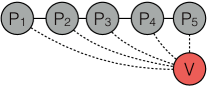
Figure 2: Illustration of $\mathcal{F}(s)$ for $n=5$. The dotted lines may or may not appear in the insertion sequence depending on the element of $S$ chosen.

The construction of $\mathcal{F}_{n}(s)$ implies an identical lower bound for the family of planar graphs, as well as interval graphs. By considering all sets $s$ of at most $k$ elements instead, we get a bound of $k\log n$ label size for any adjacency labeling scheme for $\Delta_{k}$, where $k$ is constant.

To show a similar bound on $\mathcal{T}_{k}$, we prove that the sequence of insertions creates graphs in $\mathcal{T}_{3}$. For every face $R$ in a planar embedding $M$ of a planar graph $G$, define $g(R)$ to be the minimum value of $k$, such that there is a sequence of faces $R_{0}\dots R_{k}$, with $R_{0}$ the exterior face, and $R_{k}=R$, and for $1\leq j\leq k$, there is a vertex $v$ that is both on face $R_{j-1}$ and $R_{j}$. The radius of $M$ is the minimum value of $g$ such that $g(R)\leq g$ for all regions $R$ of $M$.

Lemma 2.

[24] Let $G=(V,E)$ be a planar graph with radius $\leq g$, $g\geq 1$, then $G$ has treewidth at most $3d$.

The lemma is useful for our purposes since the graphs in the family of planar graphs resulting from $\mathcal{F}(s)$ have radius $1$.

Corollary 1.

Any dynamic adjacency labeling scheme for $\mathcal{T}_{k}$, where $k\geq 3$, requires $\Omega(n)$ bits.

4 Multi-Functional Labeling schemes

In this section we investigate labeling schemes incorporating two or more of the functions mentioned.

4.1 Dynamic Multi-Functional Labeling Schemes

A dynamic labeling scheme for answering any combination of connectivity, adjacency and sibling queries at the same time can be obtained by setting $\mathcal{L}(v)=(Id(v),Id(parent(v)),component(v))$ as described in Section 3.1 which result in a $3\log n$ labeling scheme.

We now show that this upper bound is in fact is tight. More precisely, we show that $3\log n$ bits are required to answer the combination of connectivity and adjacency. Let $I_{n}(j,k)$ be an insertion sequence designed as follows: First $j$ nodes are inserted creating an initial forest of single node trees. Then $k$ nodes are added as a path with root in the $j$th tree. At last, $n-j-k$ adjacent path leaves are added to the second-to-last node on the path. For a given $n$ we define $I_{n}$ as the family of all such insertion sequences. See Fig. 3 for reference.

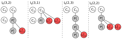
Figure 3: Illustration of $I_{n}(j,k)$ for specific values of $j$, $k$, and $n$.

Lemma 3.

Fix some dynamic labeling scheme that supports adjacency and connectivity requests. For any $1<j+k<n$, $I_{n}(k)$ must contain at least $n-j-k$ distinct labels for this labeling scheme over $I_{n}$.

The proof of Lem. 3 is found in App. 0.A.3.

Theorem 4.1.

Any dynamic labeling scheme supporting both adjacency and connectivity queries requires at least $3\log n-O(1)$ bits.

Proof.

According to Lem. 3 at least $\sum_{j=1}^{n-1}\sum_{k=1}^{n-j-1}n-j-k=\frac{1}{6}n^{3}-O(n^{2})$ distinct labels are required to label the family $I_{n}$. Thus a label size of at least $3\log n-O(1)$ bits is needed by any dynamic labeling scheme. ∎

The same family of insertion sequences can be used to show a $3\log n-O(1)$ lower bound for any dynamic labeling scheme supporting both sibling and connectivity queries. Furthermore, similarly to Theorem 3.2, the bound holds even without the assumption that the encoder is deterministic.

4.2 Static Multi-Functional labeling schemes

As seen in Thm. 4.1, the requirement to support both connectivity and adjacency force an increased label size for any dynamic labeling scheme. In this section we prove lower and upper bounds for static labeling schemes that support those operations, both for the case where the labels are necessarily unique, and for the case that they are not. From hereon, all labeling schemes are on the family of rooted forests with at most $n$ nodes.

Theorem 4.2.

Consider any function $f$ of two nodes in a single tree. If there exists an $f$-labeling scheme of size $S(n)$, where $S(n)$ is non-decreasing and $S(a)-S(b)\geq\log a-\log b-O(1)$ for any $a\geq b$. Then there exists an $f$-labeling scheme, which also supports connectivity queries of size at most $S(n)+\log\log n+O(1)$.

Proof.

We will consider the label $\mathcal{L}(v)=\{C\circ L\circ sep\}$ defined as follows. First, sort the trees of the forest according to their sizes. For the $i$th biggest tree we set $C=i$ using $\log i$ bits. Since the tree has at most $n/i$ nodes, we can pick the label $L$ internally in the tree using only $S(n/i)$ bits. Finally, we need a separator, $sep$, to separate $C$ from $L$. We can represent this using $\log\log n$ bits, since $i$ uses at most $\log n$ bits.

The total label size is this $\log i+S(n/i)+\log\log n+O(1)$ bits, which is less than $S(n)+\log\log n+O(1)$ if $S(n)-S(n/i)\geq\log i-c$ for some constant $c$, which holds by our assumption. Since $f$ is a function of two nodes from the same tree, this altered labeling scheme can answer both queries for $f$ as well as connectivity. It is now required that any label assigned has size exactly $S(n)+\log\log n$ bits, so that the decoder may correctly identify $sep$ in the bit string. For that purpose we pad labels with less bits with sufficiently many $0$’s. ∎

As a special case, we get a labeling scheme for connectivity and sibling/ancestry for $\log n+2\log\log n$ and for connectivity and sibling of $\log n+\log\log n$ if the labels need not be unique.

The following corollary is a direct result of [3, 4]. A sketch of the proof is found in App. 0.A.4.

Corollary 2.

There exists unique labeling scheme supporting both sibling and adjacency queries of size at most $\log n+2\log\log n$.

4.2.1 Lower Bound

We now show, that the upper bounds implied by Theorem 4.2 for labeling schemes supporting siblings and connectivity are indeed tight for both the unique and non-unique cases. To that end we consider the following forests: For any integers $a,b,n$ such that $ab\mid n$ denote by $F_{n}(a,b)$ a forest consisting of $a$ components (trees), each with $b$ sibling groups, where each sibling group is composed of $\frac{n}{a\cdot b}$ nodes. Note that $F_{n}(a,b)$ has at least $n$ but no more than $2n$ nodes.

Our proofs work as follows: Firstly, for any two forests $F_{n}(a,b)$ and $F_{n}(c,d)$ as defined above, we establish an upper bound on the number of labels that can be assigned to both $F_{n}(a,b)$ and $F_{n}(c,d)$. Secondly, for a carefully chosen family of forests $F_{n}(a_{1},b_{1}),\ldots,F_{n}(a_{k},b_{k})$, we show that when labeling $F_{n}(a_{i},b_{i})$ at least a constant fraction of the labels has to be distinct from the labels of $F_{n}(a_{1},b_{1}),\ldots,F_{n}(a_{i-1},b_{i-1})$. Finally, by summing over each $F_{n}(a_{i},b_{i})$ we show that a sufficiently large number of bits are required by any labeling scheme supporting the desired queries.

Our technique is a simpler version of the boxes and groups argument of Alstrup et al. [4], and generalizes to the case of two nested equivalence classes, namely connectivity and siblings. The proofs for Lem. 4 and 5 are in App. 0.A.5 and App. 0.A.6 respectively.

Lemma 4.

Let $F_{n}(a,b)$ and $F_{n}(c,d)$ be two forests such that $ab\geq cd$. Fix some unique labeling scheme supporting both connectivity and siblings, and denote the set of labels assigned to $F_{n}(a,b)$ and $F_{n}(c,d)$ as $e_{1}$ and $e_{2}$ respectively. Then

$$|e_{1}\cap e_{2}|\leq\min(a,c)\cdot\min(b,d)\cdot\frac{n}{a\cdot b}\ .$$

Lemma 5.

Let $F_{n}(a_{1},b_{1}),\ldots,F_{n}(a_{i},b_{i})$ be a family of forests with $a_{1}\cdot b_{1}\leq\ldots\leq a_{i}\cdot b_{i}$. Assume there exists a unique labeling scheme supporting both connectivity and siblings, and let $e_{j}$ denote the set of labels assigned by such a scheme to the forest $F_{n}(a_{j},b_{j})$. Assume that the sets $e_{1},\ldots,e_{i-1}$ have already been assigned. Then the number of distinct labels the encoder must introduce when assigning $e_{i}$ is at least

$$n-\sum_{j=1}^{i-1}\min(a_{j},a_{i})\cdot\min(b_{j},b_{i})\cdot\frac{n}{a_{i}\cdot b_{i}}\ .$$

We now use Lem. 5 to show the following known result [4].

Warm-up.

Any static labeling scheme for connectivity queries requires at least $\log n+\log\log n-O(1)$ bits.

Proof.

Consider the family of $\log_{3}n$ forests $F_{n}(1,1),F_{n}(3,1),\ldots,F_{n}(\log_{3}n,1)$. Since no two nodes are siblings we can use this forest combined with Lem. 5 as a lower bound for connectivity. Let $e_{j}$ denote the label set assigned by an encoder for $F_{n}(3^{j},1)$. We assume that the labels are assigned in the order $e_{0},\ldots,e_{\log_{3}n}$. By Lem. 5 the number of distinct labels introduced when assigning $e_{j}$ is at least

$$n-n\sum_{i=0}^{j-1}3^{i-j}>n/2\ .$$

It follows that labeling the $\log_{3}n$ forests in the family requires at least $\Omega(n\log n)$ distinct labels. ∎

This idea extends to some cases of non-unique labeling schemes, as seen in the theorem below. The proof of Thm. 4.3 is included in App. 0.A.7.

Theorem 4.3.

Any static labeling scheme supporting both connectivity and sibling queries requires at least $\log n+\log\log n-O(1)$ bits if the labels need not be unique.

Theorem 4.4.

Any unique static labeling scheme supporting both connectivity and sibling queries requires labels of size at least $\log n+2\log\log n-O(1)$.

Proof.

Fix some integer $x$, and assume that $n$ is a power of $x$. We consider the family of forests $F_{n}(1,1),F_{n}(x,1),F_{n}(1,x),F_{n}(x^{2},1),$ $F_{n}(x,x),F_{n}(1,x^{2}),\ldots,$$F_{n}(1,x^{\log_{x}n})$.

Let $e_{a}^{b}$ denote the label set assigned to $F_{n}(x^{a},x^{b})$ by an encoder. We assign the labels in the order $e_{0}^{0},e_{1}^{0},e_{0}^{1},e_{2}^{0},e_{1}^{1},\ldots,e_{0}^{\log_{x}n}$. Thus, when assigning $e_{a}^{b}$ we have already assigned all label sets $e_{c}^{d}$ with $c+d<a+b$ or $c+d=a+b$ and $d<b$. By Lem. 5, the number of distinct labels introduced when assigning $e_{a}^{b}$ is at least

$$n-\sum_{\begin{subarray}{c}c+d<a+b\\ c,d\geq 0\end{subarray}}\frac{n}{x^{a+b}}\cdot x^{\min(a,c)+\min(b,d)}+\sum_{d=0}^{b-1}\frac{n}{x^{a+b}}\cdot x^{a+d}\\$$

This counting argument is better demonstrated in Fig. 4. In the figure, we are concerned with assigning the labels in $e_{2}^{2}$. The grey boxes represent the label sets already assigned, and the right-side figure shows the fractions of $n$ that each set $e_{c}^{d}$ at most has in common with $e_{2}^{2}$. Observe that we can split the above sum into three cases as demonstrated in the figure: If $c\leq a$ and $d\leq b$ the bound supplied by Lem. 4 is $x^{c+d-a-b}$. Otherwise, either $c>a$ or $d>b$, but not both. If $c>a$, recall that $d<b$ so the bound is $x^{d-b}$. For $d>b$ the bound is $x^{c-a}$ by the same argument. Applying these rules, we see that the number of distinct labels introduced is at least

$$n-n\cdot\left(\sum_{c=0}^{a}\sum_{d=0}^{b}x^{c+d-a-b}+\sum_{d=0}^{b-1}(b-d)\cdot x^{d-b}+\sum_{c=0}^{a-2}(a-c)\cdot x^{c-a}\right)+n$$

$$\geq\ n-n\cdot\left(\frac{x^{2}+x+2}{(x-1)^{2}}\right)+n=n-n\cdot\frac{3x+1}{(x-1)^{2}}\ .$$

Note that we add $n$, as we have also subtracted $n$ labels for the case when $(c,d)=(a,b)$.

By setting $x=6$ we get that the encoder must introduce $6n/25$ distinct labels for each $e_{a}^{b}$. Since we have $\Theta(\log^{2}n)$ forests, a total of $\Omega(n\log^{2}n)$ labels are required for labeling the family of forests. Each forest consists of no more than $2n$ nodes, which concludes the proof. ∎

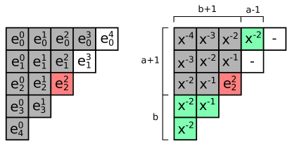
Figure 4: Demonstration of the label counting for $e_{2}^{2}$.

The same proof technique is used to prove the following theorem. For completeness, the proof is presented in Appendix 0.A.8.

Theorem 4.5.

Any unique static labeling scheme supporting both connectivity and ancestry queries requires labels of size at least $\log n+2\log\log n-O(1)$.

5 Concluding remarks

We have considered multi-functional labels for the functions adjacency, siblings and connectivity. We also provided a lower bound for ancestry and connectivity. A major open question is wether it is possible to have a label of size $\log n+O(\log\log n)$ supporting all of the functions. It seems unlikely that the best known labeling scheme for ancestry [5] can be combined with the ideas of this paper.

In the context of dynamic labeling schemes, if arbitrary node insertion is permitted, neither adjacency nor sibling labels are possible. All dynamic labeling schemes also operate when removal is allowed, simply by erasing the label to be removed. Moreover, if the tree contains not more than $n$ nodes at any moment, it is easy to show that labels of size 2 $\log n$ are necessary and sufficient for each of the functions.

Appendix 0.A Missing proofs

0.A.1 Lower bound for dynamic labeling schemes

For the function sibling we use the same family and a slightly different argument as follows. First, it again holds that $L_{1}^{k}\dots L_{n-k}^{k}$ must be different from $P_{1}\dots P_{n}$, as they are the only nodes that are siblings to $P_{k}$. Furthermore, in $F_{n}(j)$ the label $L_{i}^{j}$ (where $j>k$) is not a sibling of $P_{k}$, so $L_{i}^{j}$ must be distinct from $\{L_{1}^{k},\dots,L_{n-k}^{k}\}$.

Finally, for an identical lower bound on connectivity we define $\mathcal{F}^{c}_{n}(k)$ to be an insertion sequence of $n$ nodes, creating an initial forest of $1<k<n$ single node trees, followed by $n-k$ leaves adjacent to tree $k-1$.

0.A.2 Proof of Theorem 3.2

We prove the theorem for labeling schemes supporting adjacency requests. The proof is similar for the two other types of labeling schemes. Consider the set $F_{n}=\{\mathcal{F}_{n}(k)\mid 1<k<n/2\}$ consisting of $\Theta(n)$ different insertion sequences, and say that we uniformly choose an insertions sequence $S\in F_{n}$. Fix a deterministic labeling scheme supporting adjacency requests. Each of $\mathcal{F}_{n}(k)\in F$ has $n-k>\frac{n}{2}$ labels which are distinct for this labeling scheme over $F_{n}$ (by Lem. 1). Say that we write $F_{n}$ as $F_{n}=\{S_{1},S_{2},\ldots,S_{\left|F_{n}\right|}\}$ such that the maximal label size of the distinct labels over $F_{n}$ from $S_{i}$ is smaller than that from $S_{j}$ if $i<j$. Now consider all the labels from the insertion sequences $S_{1},\ldots,S_{i}$ which are distinct over $F_{n}$. There are at least $\frac{in}{2}$ of those meaning that at least one has label size $\log(in/2)$. This means that there is a label from $S_{i}$ which is distinct over $F_{n}$ and has label size $\geq\log n+\log i-1$. This means that the expected value of the maximal label size of $S$ (which is uniformly drawn from $F_{n}$) is at least:

$$\frac{1}{\left|F_{n}\right|}\sum_{i=1}^{\left|F_{n}\right|}\left(\log n+\log i-1\right) =(\log n-1)+\frac{1}{\left|F_{n}\right|}\left(\left|F_{n}\right|\log(\left|F_{n}\right|)-O(\left|F_{n}\right|)\right)$$

$$=\log n+\log\left|F_{n}\right|-O(1)=2\log n-O(1)$$

Since this holds for any deterministic algorithm Yao’s principle yields that for any randomized algorithm there exists $\mathcal{F}_{n}(k)\in F_{n}$ such that the expected value of the maximal label size is at least $2\log n-O(1)$ on that insertion sequence.

0.A.3 Proof of Lemma 3

Let $C_{1},\ldots,C_{n}$ be the labels of $I_{n}(n,0)$ and let $P^{j}_{1},\ldots,P^{j}_{n-j}$ be the labels of the path created by the insertion sequence $I_{n}(j,n-j)$. Since the encoder is deterministic, any insertion sequence $I_{n}(j,k)$ must assign the labels $C_{1},\ldots,C_{j}$ and $P^{j}_{1},\ldots,P^{j}_{k}$ to the first $j+k$ nodes.

Let $L^{j}_{k,i}$ denote the label of the $i$th path leaf added as a part of the insertion sequence $I_{n}(j,k)$. Clearly $L^{j}_{k,i}$ is different from any $C_{j^{\prime}}$ and $P^{j^{\prime}}_{k^{\prime}}$ by the argument of the proof of Lem. 1.

Consider now two different leaves labeled $L^{j}_{k,i}$ and $L^{j^{\prime}}_{k^{\prime},i^{\prime}}$. If $j=j^{\prime}$ and $k=k^{\prime}$ the labels must be different, as they are part of the same insertion sequence.

If $j<j^{\prime}$ then by looking at $I_{n}(j,k)$, $L^{j}_{k,i}$ and $C_{j}$ are connected. By looking at $I_{n}(j^{\prime},k^{\prime})$, $L^{j^{\prime}}_{k^{\prime},i^{\prime}}$ and $C_{j}$ are not connected. Hence the labels are different. The case $j>j^{\prime}$ is symmetric. If $j=j^{\prime}$ and $k<k^{\prime}$ then by looking at $I_{n}(j,k)$, $L^{j}_{k,i}$ and $P_{k}^{j}$ are adjacent. And from $I_{n}(j^{\prime},k^{\prime})$ we see that $L^{j^{\prime}}_{k^{\prime},i^{\prime}}$ and $P_{k}^{j}$ are not adjacent. Hence the labels are different. The case $k>k^{\prime}$ is symmetric.

In conclusion no two leaves get the same label in any of $I_{n}(j,k)$. Since $I_{n}(j,k)$ has $n-j-k$ leaves this means that $I_{n}(j,k)$ contains $n-j-k$ labels that are distinct for the labelling scheme over $I_{n}$.

0.A.4 Proof sketch for Corollary 2

It was shown in [3] how to create a labeling scheme using a recursive cluster decomposition to support adjacency in $\log n+O(\log^{*}n)$ bits. We argue that this decomposition can be combined directly with the $1$-relationship scheme of [4] to create a labeling scheme supporting both adjacency and sibling using $\log n+2\log\log n+O(\log\log\log n)$ bits.

In this proof sketch, we assume that the reader is familiar with the notations and definitions of [3, 4].

For $1$-relationship, the scheme of [4] actually works with $\log n+3\log\log n+O(1)$ bits by storing $spre(parent(v))$ for heavy nodes instead of only storing $spre(parent(v))$ for light nodes. The key is to change Lem. 4 in [4] to work for heavy nodes. This is done by considering $pre(v)-1$ instead of $pre(v)$ for heavy nodes in the proof. Since $pre(v)=spre(v)$ we can get label size $\log n+2\log\log n+O(1)$ for leaves by adding an extra flag.

The cluster decomposition used in [3] works as follows: For some integer $x$, the tree $T$ is split into $O(n/x)$ clusters of size $O(x)$. Each cluster has at most two boundary nodes, which are part of more than one cluster. We can view the clusters as a macro tree, where the nodes are the boundary nodes and the edges are the clusters. Each cluster is one of three types (see Fig. 5): Either it is a leaf cluster with just one boundary node ($\alpha$), it is a single edge ($\beta$), or it is an internal cluster with two boundary nodes ($\gamma$). Note that for $\gamma$-clusters, the top boundary node, $u$, has at most one child inside the cluster.

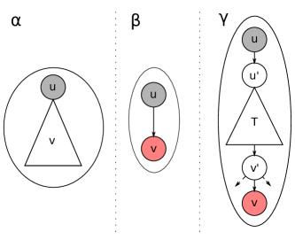
Figure 5: The three different types of clusters.

The labeling scheme works by first labeling the macro tree with the modified $1$-relationship scheme, such that the label of a cluster $C$ is denoted $\mathcal{L}^{M}(C)$. Inside each cluster the nodes are labeled, such that the label of a node $v$ is denoted by $\mathcal{L}^{C}(v)$.

A node $v$ of the original tree $T$ will be labeled the following way (refer to Fig. 5 for the node types). Note that upper boundary nodes $u$ are not included in the cluster – only lower boundary nodes.

Type-$v$ node in $\alpha$-cluster $C$:

We set $\mathcal{L}(v)=\{\mathcal{L}^{M}(C)\circ\mathcal{L}^{C}(v)\circ type\}$.

Type-$v$ node in $\beta$-cluster $C$:

We set $\mathcal{L}(v)=\{\mathcal{L}^{M}(C)\circ type\}$.

Type-$u^{\prime}$ and type-$v$ nodes in $\gamma$-cluster $C$:

We set $\mathcal{L}(u^{\prime})=\{\mathcal{L}^{M}(C)\circ type\}$ (and identical for $v$).

Type $T$ and type-$v^{\prime}$ nodes in $\gamma$-cluster $C$:

We set $\mathcal{L}(v^{\prime})=\{pre^{M}(C)\circ\mathcal{L}^{C}(v^{\prime})\circ type\}$.

The $type$ parameter is a constant number of bits specifying the following: Which cluster type is it $\{\alpha,\beta,\gamma\}$. Which type of node is it $\{$child of $u$ in $\alpha$, type $u^{\prime}$ in $\gamma$, type $v$ in $\gamma$, type $v^{\prime}$ in $\gamma$, child of $v^{\prime}$ in $\gamma$, child of $u^{\prime}$ in $\gamma$, none of the above$\}$.

The proof of correctness and label size now follows by setting $x=O(\log^{4}n)$ and the same techniques as in [3, 4], which is basically checking the cases of different pairs of node types.

0.A.5 Proof of Thorem 4

Consider label sets $s_{1}$ and $s_{2}$ of two sibling groups from $F_{n}(a,b)$ and $F_{n}(c,d)$ respectively for which $|s_{1}\cap s_{2}|\geq 1$. Clearly, we must have $|s_{1}\cap s_{2}|\leq\min(|s_{1}|,|s_{2}|)=\frac{n}{a\cdot b}$. Furthermore, no other sibling group of $F_{n}(a,b)$ or $F_{n}(c,d)$ can be assigned labels from $s_{1}\cup s_{2}$, as the sibling relationship must be maintained. We can thus create a one-to-one matching between the sibling groups of $F_{n}(a,b)$ and $F_{n}(c,d)$, that have labels in common (note that not all sibling groups will necessarily be mapped). Bounding the number of common labels thus becomes a problem of bounding the size of this matching. In order to maintain the connectivity relation, sibling groups from one component cannot be matched to several components. Therefore at most $\min(b,d)$ sibling groups can be shared per component, and at most $\min(a,c)$ components can be shared. Combining this gives the final bound of $\min(a,c)\cdot\min(b,d)\cdot\frac{n}{a\cdot b}$.

0.A.6 Proof of Theorem 5

Assume that the encoder has already assigned labels to the set $e_{i}$. The number of distinct labels of $e_{i}$ is then exactly

$$n-\left|\bigcup_{j=1}^{i-1}(e_{j}\cap e_{i})\right|\ .$$

Since $|A\cup B|\leq|A|+|B|$ this is bounded from below by

$$n-\sum_{j=1}^{i-1}|e_{j}\cap e_{i}|\geq n-\sum_{j=1}^{i-1}\min(a_{j},a_{i})\cdot\min(b_{j},b_{i})\cdot\frac{n}{a_{i}\cdot b_{i}}\ .$$

Here the inequality follows from Lem. 4

0.A.7 Proof of Theorem 4.3

The key idea is to create a family of forests, such that the non-unique case reduces to the unique case.

Proof.

Assume w.l.o.g. that $n$ is a power of $3$. Consider the family of $\log_{3}n$ forests $F_{n}(1,n),F_{n}(3,n/3),F_{n}(3^{2},n/3^{2}),\ldots,$ $F_{n}(3^{\log_{3}n},1)$. Since each sibling group of the forest $F_{n}(3^{i},n/3^{i})$ has exactly one node, we note that no two nodes are siblings. Thus each label of the forest has to be unique, since we have assumed that a node is sibling to itself. We can thus use Lem. 4 as if we were in the unique case for this family of forests.

Let $e_{j}$ denote the label set assigned by an encoder for $F_{n}(3^{j},n/3^{j})$. We assume that the labels are assigned in the order $e_{0},\ldots,e_{\log_{3}n}$. By Lem. 5 the number of distinct labels introduced when assigning $e_{j}$ is at least

$$n-n\sum_{i=0}^{j-1}3^{i-j}>n/2$$

It follows that when labeling each of the $\log_{3}n$ forests in the family, any encoder must introduce at least $n/2$ distinct labels, i.e. $\Omega(n\log n)$ distinct labels in total. The family consist of forests with no more than $2n$ nodes, which concludes the proof. ∎

0.A.8 Proof of Theorem 4.5

For integers $n,a,b$ such that $ab\mid n$, let $G_{n}(a,b)$ be a forest consisting of $a$ components consisting each of $b$ paths of length $\frac{n}{ab}$ each connected to a root in the component. Each forest in $G_{n}(a,b)$ consists of at least $n$ but no more than $2n$ nodes.

The key idea in the proof of Thm. 4.4 is the use of Lem. 4. Below we show Lem. 6 which is is analogous to Lem. 4 which derives the proof of Thm. 4.5 similarly.

Lemma 6.

Let $G_{n}(a,b)$ and $G_{n}(c,d)$ be two forests such that $ab\geq cd$. Fix some unique labeling scheme supporting both connectivity and ancestry queries, and denote the set of labels assigned to $G_{n}(a,b)$ and $G_{n}(c,d)$ as $e_{1}$ and $e_{2}$ respectively. Then

$$|e_{1}\cap e_{2}|\leq\min(a,c)\cdot\min(b,d)\cdot\frac{n}{a\cdot b}\ .$$

Proof.

Let $s_{1}$ and $s_{2}$ be the labels assigned to two paths from $G_{n}(a,b)$ and $G_{n}(a,b)$ respectively for which $s_{1}\cap s_{2}\neq\emptyset$. The number of labels the paths have in common is at most $\left|s_{1}\right|=\frac{n}{ab}$. Furthermore, no other paths from $G_{n}(a,b)$ or $G_{n}(c,d)$ can reuse any labels from $s_{1}\cup s_{2}$ since the ancestry relation has to be maintained. Therefore we can create a one-to-one matching between the paths from $G_{n}(a,b)$ and $G_{n}(c,d)$, which have at least on label in common (note that not all sibling groups will necessarily be mapped).

Bounding the number of common labels thus reduces to bounding the size of this matching. In order to maintain the connectivity relation, paths from one component cannot be matched to more than one. Therefore at most $\min(b,d)$ paths can be shared per component, and at most $\min(a,c)$ components can be shared. Combining this gives the final bound of $\min(a,c)\cdot\min(b,d)\cdot\frac{n}{a\cdot b}$. ∎

References

- [1] M. A. Breuer, J. Folkman, An unexpected result in coding the vertices of a graph, J. Mathematical Analysis and Applications 20 (1967) 583–600.
- [2] S. Kannan, M. Naor, S. Rudich, Implicit representation of graphs, in: SIAM Journal On Discrete Mathematics, 1992, pp. 334–343.
- [3] S. Alstrup, T. Rauhe, Small induced-universal graphs and compact implicit graph representations, in: FOCS ’02, 2002, pp. 53–62.
- [4] S. Alstrup, P. Bille, T. Rauhe, Labeling schemes for small distances in trees, SIAM J. Discret. Math. 19 (2) (2005) 448–462.
- [5] P. Fraigniaud, A. Korman, An optimal ancestry scheme and small universal posets, in: STOC ’10, STOC ’10, 2010, pp. 611–620.
- [6] S. Alstrup, E. B. Halvorsen, K. G. Larsen, Near-optimal labeling schemes for nearest common ancestors, in: SODA, 2014, pp. 972–982.
- [7] M. Thorup, U. Zwick, Compact routing schemes, in: SPAA ’01, 2001, pp. 1–10.
- [8] D. Peleg, Proximity-preserving labeling schemes, Journal of Graph Theory 33 (3) (2000) 167–176.
- [9] X. Wu, M. L. Lee, W. Hsu, A prime number labeling scheme for dynamic ordered xml trees, in: Data Engineering, 2004. Proceedings. 20th International Conference on, IEEE, 2004, pp. 66–78.
- [10] M. Lewenstein, J. I. Munro, V. Raman, Succinct data structures for representing equivalence classes, in: Algorithms and Computation, Springer, 2013, pp. 502–512.
- [11] E. Cohen, H. Kaplan, T. Milo, Labeling dynamic xml trees, SIAM Journal on Computing 39 (5) (2010) 2048–2074.
- [12] P. Fraigniaud, C. Gavoille, Routing in trees, in: ICALP ’01, Springer, 2001, pp. 757–772.
- [13] A. Korman, D. Peleg, Y. Rodeh, Labeling schemes for dynamic tree networks, Theory of Computing Systems 37 (1) (2004) 49–75.
- [14] A. Korman, General compact labeling schemes for dynamic trees, Distributed Computing 20 (3) (2007) 179–193.
- [15] A. Korman, D. Peleg, Labeling schemes for weighted dynamic trees, Information and Computation 205 (12) (2007) 1721–1740.
- [16] A. Korman, Improved compact routing schemes for dynamic trees, in: PODC ’08, ACM, 2008, pp. 185–194.
- [17] A. Korman, Compact routing schemes for dynamic trees in the fixed port model, Distributed Computing and Networking (2009) 218–229.
- [18] N. Rotbart, M. Vas Salles, I. Zotos, An evaluation of dynamic labeling schemes for tree networks, SEA ’14, 2014.
- [19] D. Peleg, Informative labeling schemes for graphs, Theor. Comput. Sci. 340 (3) (2005) 577–593.
- [20] A. C.-C. Yao, Probabilistic computations: Toward a unified measure of complexity, in: FOCS 77, IEEE Computer Society, Washington, DC, USA, 1977, pp. 222–227.
- [21] C. Gavoille, A. Labourel, Shorter implicit representation for planar graphs and bounded treewidth graphs, in: Algorithms–ESA 2007, Springer, 2007, pp. 582–593.
- [22] F. R. Graham Chung, Universal graphs and induced-universal graphs, Journal of Graph Theory 14 (4) (1990) 443–454.
- [23] D. Adjiashvili, N. Rotbart, Labeling schemes for bounded degree graphs, ICALP ’14, 2014.
- [24] H. L. Bodlaender, Dynamic programming on graphs with bounded treewidth, Springer, 1988.