The Panchromatic Hubble Andromeda Treasury. VI. The reliability of far-ultraviolet flux as a star formation tracer on sub-kpc scales.

Abstract

We have used optical observations of resolved stars from the Panchromatic Hubble Andromeda Treasury (PHAT) to measure the recent ($<500\,\mathrm{Myr}$) star formation histories (SFHs) of 33 FUV-bright regions in M31. The region areas ranged from $\sim 10^{4}$ to $10^{6}\,\mathrm{pc}^{2}$, which allowed us to test the reliability of FUV flux as a tracer of recent star formation on sub-kpc scales. The star formation rates (SFRs) derived from the extinction-corrected observed FUV fluxes were, on average, consistent with the 100-Myr mean SFRs of the SFHs to within the $1-\sigma$ scatter. Overall, the scatter was larger than the uncertainties in the SFRs and particularly evident among the smallest regions. The scatter was consistent with an even combination of discrete sampling of the initial mass function and high variability in the SFHs. This result demonstrates the importance of satisfying both the full-IMF and the constant-SFR assumptions for obtaining precise SFR estimates from FUV flux. Assuming a robust FUV extinction correction, we estimate that a factor of 2.5 uncertainty can be expected in FUV-based SFRs for regions smaller than $10^{5}\,\mathrm{pc}^{2}$, or a few hundred pc. We also examined ages and masses derived from UV flux under the common assumption that the regions are simple stellar populations (SSPs). The SFHs showed that most of the regions are not SSPs, and the age and mass estimates were correspondingly discrepant from the SFHs. For those regions with SSP-like SFHs, we found mean discrepancies of $10\,\mathrm{Myr}$ in age and a factor of 3 to 4 in mass. It was not possible to distinguish the SSP-like regions from the others based on integrated FUV flux.

1. Introduction

A common technique for estimating global star formation rates (SFRs) in individual galaxies is to measure the total flux at wavelengths known to trace recent star formation (SF), such as ultraviolet (UV) emission from intermediate- and high-mass stars. After correcting for dust extinction, an observed flux can be converted into a SFR using a suitable calibration, which is typically a linear scaling of intrinsic luminosity derived from population synthesis modeling. The modeling process requires a set of stellar evolution models and a stellar initial mass function (IMF), as well as a characterization of the star formation history (SFH; the evolution of SFR over time) and the metallicity of the population. These quantities are often not well-constrained for a given system and need to be assumed (see reviews by Kennicutt 1998, Kennicutt & Evans 2012, and references therein).

A set of flux calibrations widely used in extragalactic studies were presented by Kennicutt (1998, see , for updates). These calibrations are based on models of a generic population with solar metallicity, a fully populated IMF, and a SFR that has been constant over the lifetime of the tracer emission ($\sim 100\,\mathrm{Myr}$ for UV). The flux calibrations are therefore applicable to any population that can be assumed to approximate the generic population, such as spiral galaxies. In environments with low total SF (i.e., low mass) or on subgalactic scales, however, the assumptions of a fully populated IMF and a constant SFR start to become tenuous. As a result, applying the flux calibrations in these situations can lead to inaccurate SFR estimates.

For populations located within a few Mpc, it is possible to measure SFRs more directly by fitting the color magnitude diagram (CMD) of the resolved stars to obtain a SFH (Dolphin, 2002). At its core, CMD fitting is a population synthesis technique just like flux calibration (albeit much more complex) and thus requires a set of stellar evolution models, an IMF, and an accounting of dust. The primary advantage of CMD fitting over the flux calibration method for obtaining SFRs, however, is the elimination of assumptions about the SFH and metallicity. CMD-based SFHs thus provide a relative standard for testing the accuracy of SFR estimates from commonly used flux calibrations, especially in applications where the underlying full-IMF and constant-SFR assumptions are not strictly satisfied. More generally, the SFHs can be used to test results from any other flux-based method, such as ages and masses derived under the simple stellar population (SSP) assumption.

With recent Hubble Space Telescope (HST) observations from the Panchromatic Hubble Andromeda Treasury (PHAT; Dalcanton et al., 2012), we have measured the recent SFHs ($<500\,\mathrm{Myr}$) of 33 UV-bright regions in M31 and compared them with SFRs derived from UV flux. We also compared the SFHs with ages and masses derived from UV flux by treating the regions as SSPs. The UV-bright regions were cataloged by Kang et al. (2009, K09 hereafter) using Galaxy Evolution Explorer (GALEX) far-UV (FUV) flux and have areas ranging from $10^{4}$ to $10^{6}\,\mathrm{pc}^{2}$. This range of sizes allows us to test the reliability of the full-IMF, constant-SFR, and SSP assumptions on sub-kpc scales.

This paper is organized as follows. We describe our sample of UV-bright regions and show their CMDs from the PHAT photometry in §2. We summarize the CMD-fitting process, describe our extinction model, and present the resulting SFHs of the regions in §3. §4 describes the modeling of UV magnitudes from the SFHs, and §5 describes the total masses and the mean SFRs from the SFHs, as well as the SFRs based on UV flux. In §6, we compare the UV flux-based SFRs, ages, and masses with the results from the SFHs, discuss the applicability of the full-IMF, constant-SFR, and SSP assumptions to our sample, and attempt to quantify the uncertainties associated with using UV flux to estimate SFRs, ages, and masses for sub-kpc UV-bright regions.

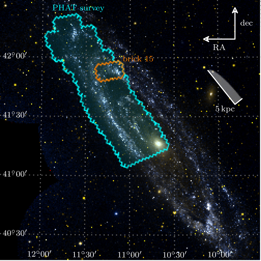
Figure 1.— Two-color composite mosaic of M31 from the GALEX Deep Imaging Survey (FUV in blue, NUV in orange). The HST/ACS outlines of the PHAT survey area and Brick 15 are highlighted in blue and orange, respectively. Brick 15 covers a portion of the 10-kpc star-forming ring. The scale bar indicates a distance of $5\;\mathrm{kpc}$ along both the major and minor axes of M31 assuming an inclination of $78\;\mathrm{deg}$ (Tully, 1994).

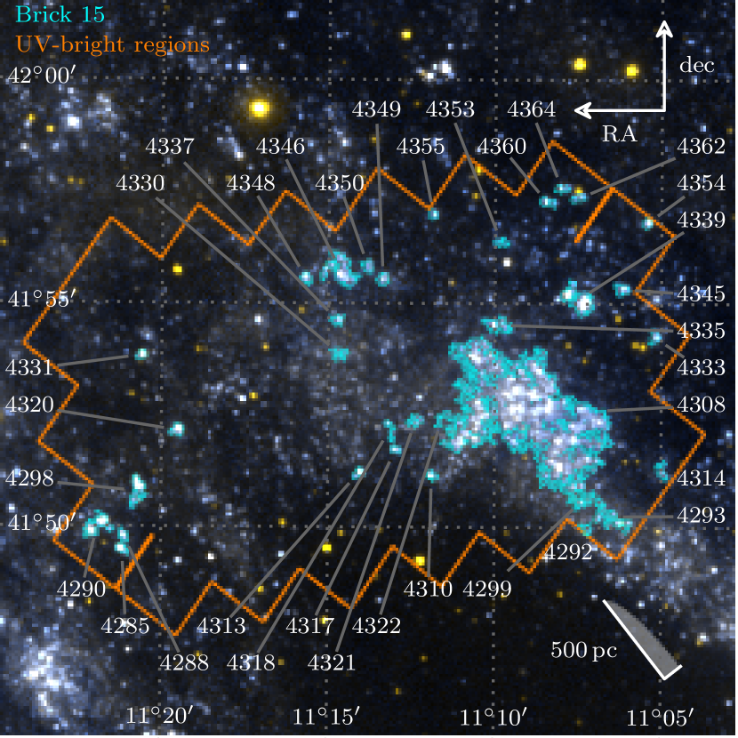
Figure 2.— Closeup of Brick 15 from the same image in Figure 1. Brick 15 contains 33 of the UV-bright regions from the Kang et al. (2009) catalog, highlighted in blue and labeled by ID number (see Table 1). The region areas, deprojected assuming an inclination of $78\;\mathrm{deg}$ (Tully, 1994), range from $\sim 10^{4}$ to $10^{6}\;\mathrm{pc}^{2}$. The scale bar indicates a distance of $500\;\mathrm{pc}$ along both the major and minor axes of M31.

2. Observations and photometry

2.1. UV-Bright Regions in M31

A set of UV-bright regions in M31 were defined by K09 using FUV ($\lambda\sim 1540\,\textrm{\AA}$) observations from GALEX. To summarize, K09 defined a region as any area covering at least 50 contiguous pixels ($113\,\mathrm{arcsec}^{2}$) with FUV surface brightness $\lesssim 25.9\,\mathrm{mag}\,\mathrm{arcsec}^{-2}$ (AB mag). For our sample, we selected the subset of these regions that were within “Brick 15” of the PHAT survey, a 0.15-deg² area consisting of 18 individual fields, or HST pointings, covering the 10-kpc star-forming ring (Figures 1 and 2). Of all the bricks comprising the PHAT survey area, Brick 15 contains the greatest amount of SF and the largest number regions – 33 total, with respect to the combined outline of its Advanced Camera for Surveys (ACS) images.

The identification numbers and locations of the regions in our sample as reported in K09 are given in Table 1. For each region, K09 measured the integrated FUV and NUV (near-UV, $\lambda\sim 2320\,\textrm{\AA}$) magnitudes and subtracted the local background estimated within a concentric annulus. We list the observed, background-subtracted FUV magnitudes, $\mathrm{FUV_{obs}}$, and UV colors, $\mathrm{(FUV-NUV)_{obs}}$ in Table 1. Table 1 also lists the solid angles and deprojected physical areas of the regions, which we calculated assuming a distance to M31 of $785\,\mathrm{kpc}$ (McConnachie et al., 2005) and a disk inclination of $78\,\mathrm{deg}$ (Tully, 1994). The areas range from $7.9\times 10^{3}$ to $7.3\times 10^{4}\,\mathrm{pc}^{2}$, with one large outlier at $1.5\times 10^{6}\,\mathrm{pc}^{2}$ (region 4308).

Table 1Observational properties of UV-bright regions in PHAT Brick 15.

ID	RA	dec	area	area	$\mathrm{FUV_{obs}}$	$\mathrm{(FUV-NUV)_{obs}}$
	(deg)	(deg)	($10^{2}\,\mathrm{arcsec}^{2}$)	($10^{3}\,\mathrm{pc}^{2}$)	(AB mag)	(AB mag)
4285*	11.352559	41.824921	001.6	0011.2	$18.570\pm 0.017$	$\phantom{+}0.325\pm 0.019$
4288*	11.352191	41.830040	001.5	0010.3	$19.281\pm 0.025$	$\phantom{+}0.147\pm 0.029$
4290*	11.364936	41.833477	005.6	0038.7	$17.377\pm 0.010$	$\phantom{+}0.468\pm 0.011$
4292*	11.120670	41.833038	001.2	0008.4	$20.457\pm 0.052$	$-0.120\pm 0.064$
4293*	11.108700	41.837337	006.5	0045.1	$18.160\pm 0.016$	$\phantom{+}0.388\pm 0.018$
4298*	11.345233	41.845989	004.9	0033.7	$17.859\pm 0.013$	$\phantom{+}0.253\pm 0.015$
4299*	11.123035	41.843586	003.0	0020.9	$19.319\pm 0.030$	$\phantom{+}0.087\pm 0.035$
4308*	11.152348	41.874954	216.5	1502.3	$13.898\pm 0.002$	$\phantom{+}0.181\pm 0.002$
4310*	11.197878	41.852535	001.2	0008.2	$19.411\pm 0.027$	$\phantom{+}0.303\pm 0.030$
4313*	11.234838	41.853275	001.5	0010.3	$19.026\pm 0.022$	$\phantom{+}0.290\pm 0.025$
4314*	11.082835	41.854801	001.8	0012.2	$19.714\pm 0.032$	$\phantom{+}0.115\pm 0.037$
4317*	11.216114	41.862221	001.1	0007.9	$19.556\pm 0.029$	$\phantom{+}0.259\pm 0.033$
4318*	11.218816	41.869392	001.3	0008.9	$19.978\pm 0.038$	$-0.058\pm 0.045$
4320*	11.325653	41.868969	002.1	0014.8	$18.200\pm 0.014$	$\phantom{+}0.195\pm 0.016$
4321*	11.206724	41.872875	001.8	0012.8	$19.823\pm 0.037$	$\phantom{+}0.118\pm 0.043$
4322*	11.193023	41.873569	001.2	0008.2	$20.810\pm 0.067$	$-0.164\pm 0.085$
4330*	11.244569	41.897583	002.1	0014.7	$19.848\pm 0.039$	$\phantom{+}0.087\pm 0.046$
4331	11.343492	41.897060	001.3	0009.1	$18.411\pm 0.016$	$\phantom{+}0.462\pm 0.017$
4333	11.086989	41.904243	001.8	0012.5	$18.811\pm 0.019$	$-0.271\pm 0.023$
4335*	11.165060	41.908730	004.6	0032.0	$18.172\pm 0.016$	$\phantom{+}0.026\pm 0.018$
4337*	11.245595	41.910343	001.7	0011.6	$19.294\pm 0.026$	$\phantom{+}0.014\pm 0.031$
4339*	11.125310	41.918499	009.5	0066.0	$16.591\pm 0.007$	$\phantom{+}0.087\pm 0.008$
4345	11.103488	41.922085	002.3	0015.8	$18.625\pm 0.018$	$-0.182\pm 0.022$
4346*	11.244633	41.928699	010.5	0073.0	$17.194\pm 0.010$	$-0.007\pm 0.012$
4348*	11.261269	41.925659	001.6	0011.4	$18.717\pm 0.019$	$-0.129\pm 0.022$
4349*	11.222815	41.925503	001.9	0012.9	$19.313\pm 0.026$	$\phantom{+}0.248\pm 0.030$
4350*	11.230723	41.930325	001.6	0011.2	$19.514\pm 0.030$	$\phantom{+}0.062\pm 0.034$
4353*	11.163334	41.939396	001.2	0008.5	$20.168\pm 0.040$	$-0.241\pm 0.049$
4354*	11.090720	41.946636	001.3	0008.9	$18.454\pm 0.016$	$\phantom{+}0.037\pm 0.018$
4355	11.197759	41.949593	001.1	0007.9	$19.008\pm 0.021$	$-0.289\pm 0.025$
4360	11.140469	41.954372	001.8	0012.8	$18.533\pm 0.017$	$-0.256\pm 0.020$
4362	11.125412	41.955841	001.5	0010.6	$19.363\pm 0.026$	$-0.010\pm 0.030$
4364*	11.133373	41.959290	001.4	0009.7	$19.342\pm 0.025$	$\phantom{+}0.122\pm 0.029$
comb.			083.6	0580.3	$14.764\pm 0.003$	$\phantom{+}0.139\pm 0.004$

2.2. PHAT photometry

The resolved star photometry used in this study was taken from the PHAT Year 1 data release (Dalcanton et al., 2012). The PHAT photometric catalogs were generated using DOLPHOT, a version of HSTPHOT (Dolphin, 2000) with added ACS- and Wide Field Camera 3-specific modules. Although the wavelength coverage of PHAT extends from the UV to the near-infrared, we have used only the ACS optical images (F475W and F814W filters) since they contain the greatest numbers of stars and reach the deepest CMD features of the three PHAT cameras.

We applied quality cuts to the raw ACS photometric catalogs to minimize non-stellar contaminants in our CMDs. Specifically, we required that each object meet the following restrictions: $\mathtt{SNR}_{\mathrm{F475W}}\geq 4$, $\mathtt{SNR}_{\mathrm{F814W}}\geq 4$, $(\mathtt{sharp}_{\mathrm{F475W}}^{2}+\mathtt{sharp}_{\mathrm{F814W}}^{2})\leq 0.075$, and $(\mathtt{crowd}_{\mathrm{F475W}}^{2}+\mathtt{crowd}_{\mathrm{F814W}}^{2})\leq 1.0$, where $\mathtt{SNR}$, $\mathtt{sharp}$, and $\mathtt{crowd}$ refer to the DOLPHOT signal-to-noise, sharpness, and crowding parameters in each filter. These quality cuts are the “gst” cuts outlined in the main PHAT data release (Dalcanton et al., 2012).

We extracted all stars within the boundaries of the 33 UV-bright regions, combining photometry as needed for regions extending across multiple ACS fields. We did not take advantage of the improved signal-to-noise ratio where fields overlapped. The CMDs of the Brick 15 UV-bright regions are shown in Figure 3.

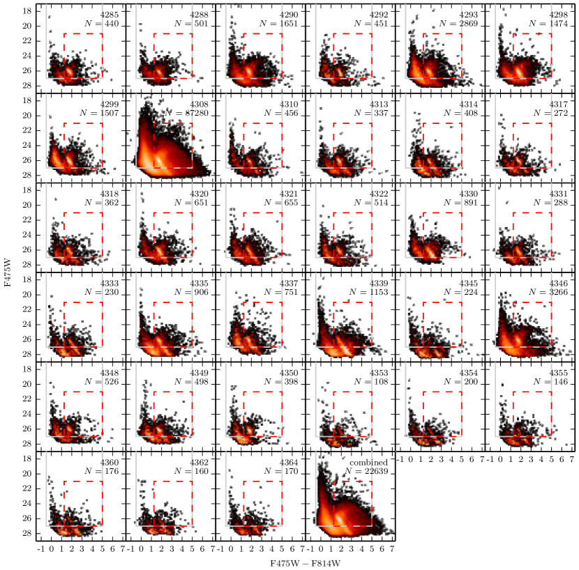
Figure 3.— Optical color-magnitude diagrams (ACS/WFC filters F475W and F814W) of the UV-bright regions. Region ID numbers and the numbers of stars fit by MATCH are shown in each panel. The MATCH fit area is inside the solid gray line, where the faint end marks the 50% completeness limit in F475W. Stars within the red dashed line were excluded from the fit. The combined region includes all regions except 4308. The CMDs show broadening of the main sequence and other features, indicating that the regions are subject to nontrivial amounts of differential extinction from dust internal to M31.

2.3. Artificial star tests

To assess observational errors and characterize photometric completeness, we conducted $\sim 2.5\times 10^{4}$ artificial star tests (ASTs) for each of the regions. The color and magnitude distributions for the ASTs were modeled after the CMDs of the individual regions. However, as discussed below in §3.2, we excluded the red giant branch (RGB) and red clump (RC) from the SFH analysis. We therefore only considered ASTs with properties similar to the blue portion of the CMDs, including the luminous main sequence (MS).

We used the ASTs to compute the photometric completeness functions for each of the 33 regions. The completeness functions were consistent throughout the sample, with an uncertainty of $0.06\,\mathrm{mag}$ in the mean 50% completeness limit in each filter. In addition, the photometric errors varied little between the regions. These consistencies allowed us to combine the ASTs from the individual regions for a total of $1.6\times 10^{6}$ ASTs. This hundredfold increase in the number of ASTs available to each region provided a superior CMD error model for the SFH measurement process. The 50% completeness limits of the region sample are $27.0\,\mathrm{mag}$ in F475W and $26.2\,\mathrm{mag}$ in F814W.

3. The recent SFHs of UV-bright regions in M31

The derivation of the SFHs for the UV-bright regions is described in this section. The first subsection gives a brief discussion of the SFH code and describes the overall SFH measurement procedure from beginning to end. Details of the extinction model, the resulting SFHs, and our uncertainty analysis are discussed in the subsequent subsections.

3.1. CMD modeling with MATCH

We used the SFH code MATCH (Dolphin, 2002) to measure the SFHs of our sample of UV-bright regions. Assuming a stellar IMF, binary fraction, and a set of stellar evolution models, MATCH constructs a series of synthetic CMDs over given ranges in distance, age, metallicity, and extinction. The synthetic CMDs are convolved with the error model from the ASTs to account for observational errors. Linear combinations of the synthetic CMDs form a model which is assigned a fit value based on a comparison with the observed CMD. The SFH of the model CMD that minimizes the fit value is considered the most likely SFH of the observed population given the input parameters. We emphasize that MATCH models the distribution of stars in the observed CMD, not the ages and masses of the individual stars.

The fit statistic used by MATCH is equal to $-2\ln\Lambda_{P}$, where $\Lambda_{P}$ is the Poisson likelihood ratio. According to Wilks’ theorem, this statistic is asymptotically $\chi^{2}$ distributed, allowing us to estimate the $n\sigma$ confidence limits in a set of SFH solutions using the condition $\mathrm{fit-fit_{min}}\leq n^{2}$, where $\mathrm{fit_{min}}$ corresponds to the best-fit SFH. This method was used to estimate various uncertainties in §3.3 and §3.4.

We assumed the following for our SFH measurements:

1. A Kroupa IMF (Kroupa, 2001).

2. The Padova stellar evolution models for masses between 0.15 and $120\,M_{\odot}$ (the IMF was normalized using masses down to $0.01\,M_{\odot}$) including updated low-mass asymptotic giant branch tracks (Girardi et al., 2010).

3. A binary fraction of 0.35 with a uniform secondary mass distribution.

4. A distance modulus of 24.47 (McConnachie et al., 2005). The distance to M31 is fairly well-known, allowing us to fix this value and eliminate a free parameter in the CMD fitting process.

5. A set of 48 log-spaced age bins from $\log_{10}(\mathrm{Age/yr})=6.60$ to $9.00\,\mathrm{dex}$ with width $\Delta\log_{10}(\mathrm{Age/yr})=0.05\,\mathrm{dex}$ (though as discussed in §3.3, we ultimately only consider the SFH out to $500\,\mathrm{Myr}$, or $\log_{10}(\mathrm{Age/yr})=8.70$).

6. A metallicity range of $[\mathrm{M/H}]=-2.3$ to $0.1\,\mathrm{dex}$ at a resolution of $0.1\,\mathrm{dex}$ with the requirement of a monotonically increasing chemical evolution model.

We also simulated the effects of intervening Galactic foreground populations using the TRILEGAL population synthesis model (Girardi et al., 2005). The solid angles of the regions were small enough, however, that no more than a few foreground stars were expected per CMD, implying a negligible impact on our final results.

Extinction was modeled using two parameters, $A_{\mathrm{V}f}$ and $dA_{\mathrm{V}}$, as described in §3.2. For each region, we sampled the extinction parameter surface using a combination of pattern search and grid search techniques, measuring the best-fit SFH at each point. The search procedure resulted in an irregularly-sampled grid of MATCH fit values with a minimum step size of $0.05\,\mathrm{mag}$ in both $A_{\mathrm{V}f}$ and $dA_{\mathrm{V}}$. We then compared the fit values across the grid to find the overall best-fit SFH. Figure 4 shows an example model CMD for the best-fit SFH of region 4339, along with the observed CMD and the residual significance.

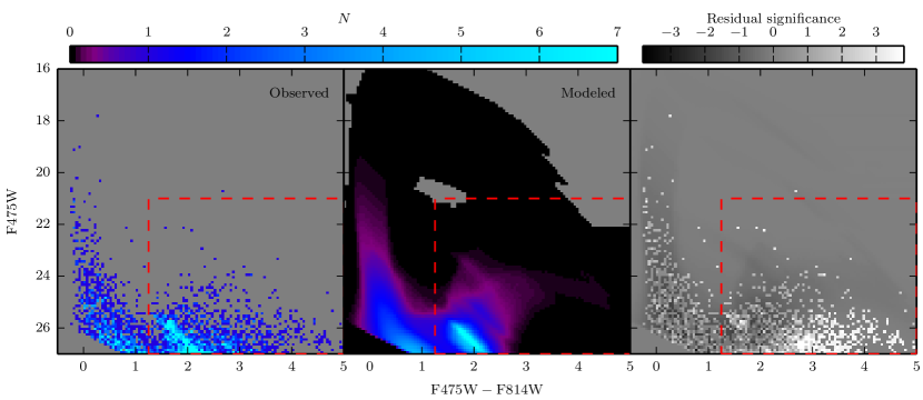
Figure 4.— Observed CMD of region 4339, with the best-fit modeled CMD and the residual significance (the observed CMD minus the modeled CMD, weighted by the variance). The color maps indicate the number of stars in each color and magnitude bin. The CMD limits correspond to the solid gray lines shown in Figure 3, and the dashed red line shows the area excluded from the fitting process. We find no systematic residuals in the MS, indicating that the model is a good fit to the data.

3.2. Extinction model

K09 measured the average $E(\mathrm{B-V})$ reddening in each region using the reddening-free parameter $Q$ and UBV photometry for individual OB stars, providing us with possible constraints on extinction for CMD fitting with MATCH. However, the CMDs in Figure 3 show broadening of the intrinsically narrow MS, indicating that the regions are subject to nontrivial amounts of differential extinction from dust internal to M31. In some regions the differential extinction is severe enough that the MS appears doubled. Differential extinction is also evident in the population of older stars, which we assume to be reasonably well-mixed throughout the galaxy, characterized by a broad RGB and an elongation of the RC along the reddening vector. These complexities lead to poor results when fitting an entire CMD with a single extinction value, such as that obtained from the average $E(\mathrm{B-V})$ in a region.

To fit the CMDs more accurately, we adopted a two-parameter extinction model consisting of a foreground dust component and a differential component. The total V-band extinction common to all stars in the CMD is set by the foreground parameter, $A_{\mathrm{V}f}$. Differential extinction is added to the stars in varying amounts following a uniform distribution from zero up to a maximum determined by the differential parameter, $dA_{\mathrm{V}}$. Compared to the simplest case of optimizing a single extinction parameter, this extinction model provided much better fits for the observed CMDs while allowing MATCH to compute best-fit SFH solutions in a reasonable amount of time.

A specific shortcoming of the model, however, is that not all populations are expected to have the same extinction profile. Young stars tend to reside closer to the midplane of the galaxy and are likely to be physically associated with cold dense gas that hosts the dusty ISM. The older RGB and RC stars, which dominate the CMDs of the regions, can have a much larger scale height in comparison. To prevent the older populations from influencing the parameters of the extinction model we excluded all stars with both $\mathrm{F475W-F814W}>1.25$ and $\mathrm{F475W}>21.0\,\mathrm{mag}$ (red dashed lines in Figure 3) from the CMD fitting process. The SFHs and extinction parameters we derive from MATCH therefore correspond only to the distributions of massive MS stars (the primary producers of UV flux) as well as any blue and red He-burning stars in the CMDs.

By creating an exclusion area in the CMD, we necessarily place a limit on the total extinction that can be determined by MATCH. From the CMDs in Figure 3, the maximum amount of reddening a MS star can have before entering the exclusion area is $\mathrm{F475W-F814W}\approx 1.7\,\mathrm{mag}$. Assuming the extinction curve from Cardelli et al. (1989, see §6.1), this amount of reddening corresponds to a total extinction of $A_{\mathrm{V}f}+dA_{\mathrm{V}}\approx 2.8\,\mathrm{mag}$. CMD models with total extinction at this limit are indistinguishable from higher-extinction models because stars in the exclusion area do not affect the MATCH fit statistic. We therefore place an upper limit of $2.8\,\mathrm{mag}$ on the total extinction, $A_{\mathrm{V}f}+dA_{\mathrm{V}}$, during the optimization of the SFHs described in §3.1.

One caveat for our two-component model is that observational studies of the ISM routinely demonstrate log-normal, not uniform, density distributions (e.g., Berkhuijsen & Fletcher, 2008; Hill et al., 2008; Ballesteros-Paredes et al., 2011; Shetty et al., 2011; Dalcanton et al., 2014). Modeling the extinctions in M31 with log-normal distributions has been successful for producing extinction maps that agree with the emission from dust and gas (Dalcanton et al., 2014). Implementing such a model in MATCH would require a minimum of three parameters: a foreground component, and the mean and variance for the log-normal. A more realistic extinction model might account for the fraction of stars affected by the log-normal as well as the scale height of the stars relative to the gas in the disk, which can vary with age. With each additional parameter, however, the size of the search space increases exponentially and measuring the SFH of a single region quickly becomes impractical. It is difficult to assess how the derived SFHs are affected by our comparatively simple extinction model without repeating the measurements with a more sophisticated model. Even so, the quality of the residuals for the modeled CMDs (e.g., Figure 4) suggests that the two-component model is reasonably accurate.

3.3. Results

We present the SFHs of the UV-bright regions in Figure 5. The corresponding best-fit $A_{\mathrm{V}f}$ and $dA_{\mathrm{V}}$ parameters are listed in Table 2. The uncertainties of the parameters for each region correspond to the minimum and maximum values among the set of SFHs within $1\sigma$ of the best-fit SFH on the $A_{\mathrm{V}f},dA_{\mathrm{V}}$ surface (i.e., all SFHs for which $\mathrm{fit-fit_{min}}\leq 1$; see §3.1). The final metallicities of the best-fit SFHs for all regions ranged from $-1.30\,\mathrm{dex}\leq[{\rm M/H}]\leq 0.01\,\mathrm{dex}$, with 80% of the values within $0.3\,\mathrm{dex}$ of the mean, $[{\rm M/H}]=-0.3\,\mathrm{dex}$.

The exclusion area in the CMDs and the 50% photometric completeness limit both restrict the age of the oldest population that can be fit by MATCH. Through synthetic CMD modeling, we find that a significant fraction of the stars in populations older than $\sim 500\,\mathrm{Myr}$ are either within the exclusion area or below the 50% photometric completeness limit. In comparison, younger populations are well-represented in the MS/He-burning area of the CMD. We therefore adopt $500\,\mathrm{Myr}$ as the maximum reliable age of the SFHs.

Considering that the UV emission from an SSP becomes negligible after $\sim 100\,\mathrm{Myr}$ (Gogarten et al., 2009; Leroy et al., 2012), we chose to display only the past $200\,\mathrm{Myr}$ of the SFHs. This was done to show as much of the overall history as possible while preserving sufficient detail in the $0-100\,\mathrm{Myr}$ range. Also, the SFHs are shown at a coarser time resolution than the actual resolution of $\Delta\log_{10}(\mathrm{Age/yr})=0.05\,\mathrm{dex}$ to simplify visual comparisons between the regions. We use the full-resolution SFHs for all analyses that follow.

The Padova stellar evolution models used to fit the CMDs do not include ages less than $4\,\mathrm{Myr}$, creating a gap between the present time and the youngest age bin in the SFHs. To account for this, we extended the youngest bin to cover the ages in the gap and rescaled its SFR such that the total mass formed in the bin was conserved.

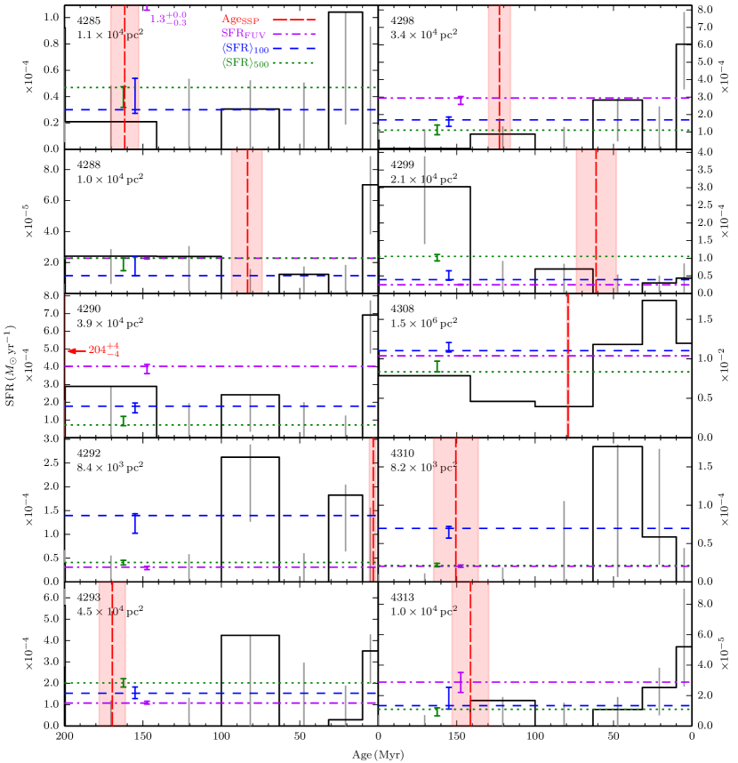
Figure 5.— SFHs of UV-bright regions in M31 (black histogram). The SFH for the combined region in Figure 3 was derived independently. The region ID number and deprojected area are given in each panel. The vertical long-dashed red line shows $\mathrm{Age_{SSP}}$, the SSP age from Kang et al. (2009), which does not accurately describe the majority of the SFHs. The dashed-dotted purple line shows the constant SFR, $\mathrm{SFR_{FUV}}$, obtained from the extinction-corrected observed FUV fluxes. The short-dashed blue and dotted green lines show $\langle\mathrm{SFR}\rangle_{100}$ and $\langle\mathrm{SFR}\rangle_{500}$, the mean SFRs over the last 100 and $500\,\mathrm{Myr}$, respectively.

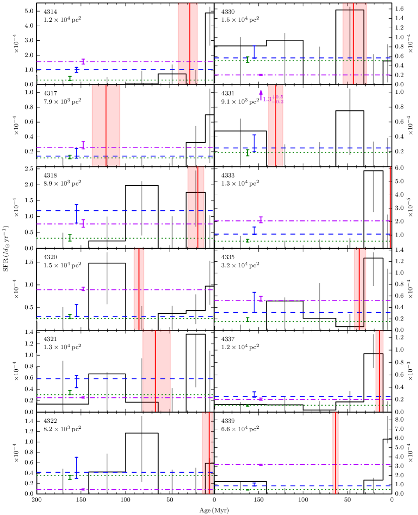
Figure 5.— Cont.

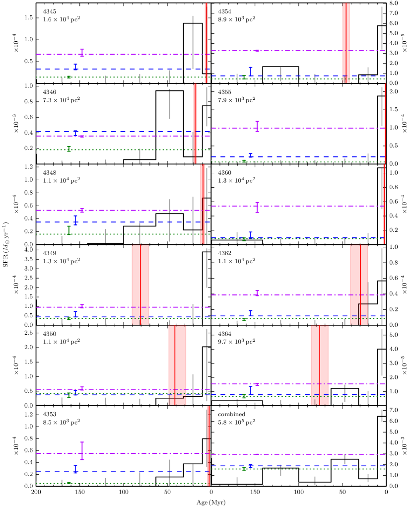
Figure 5.— Cont.

Table 2Region properties derived from the SFHs.

ID	$A_{\mathrm{V}f}$	$dA_{\mathrm{V}}$	$M_{100}$, $\langle\mathrm{SFR}\rangle_{100}$	$M_{\mathrm{peak}}$	$M_{\mathrm{peak}}/M_{100}$	$\mathrm{Age_{peak}}$
			$(10^{3}\,M_{\odot}$, $10^{-5}\,M_{\odot}\,\mathrm{yr}^{-1})$	$(10^{3}\,M_{\odot})$		(Myr)
4285*	$0.30\begin{subarray}{c}+0.00\\ -0.05\end{subarray}$	$2.50\begin{subarray}{c}+0.05\\ -0.25\end{subarray}$	$\phantom{0}\phantom{0}\phantom{0}3.0\begin{subarray}{c}+2.4\phantom{0}\phantom{0}\\ -0.3\phantom{0}\phantom{0}\end{subarray}$	$\phantom{0}\phantom{0}\phantom{0}2.4\begin{subarray}{c}+0.0\phantom{0}\phantom{0}\\ -1.8\phantom{0}\phantom{0}\end{subarray}$	0.78	$23.8\begin{subarray}{c}+52.3\\ -8.8\phantom{0}\end{subarray}$
4288*	$0.60\begin{subarray}{c}+0.00\\ -0.00\end{subarray}$	$0.00\begin{subarray}{c}+0.00\\ -0.00\end{subarray}$	$\phantom{0}\phantom{0}\phantom{0}1.2\begin{subarray}{c}+1.2\phantom{0}\phantom{0}\\ -0.0\phantom{0}\phantom{0}\end{subarray}$	$\phantom{0}\phantom{0}\phantom{0}0.6\begin{subarray}{c}+0.0\phantom{0}\phantom{0}\\ -0.3\phantom{0}\phantom{0}\end{subarray}$	0.54	$\phantom{0}6.7\begin{subarray}{c}+54.0\\ -4.3\phantom{0}\end{subarray}$
4290*	$0.40\begin{subarray}{c}+0.00\\ -0.05\end{subarray}$	$1.95\begin{subarray}{c}+0.30\\ -0.05\end{subarray}$	$\phantom{0}\phantom{0}17.8\begin{subarray}{c}+1.8\phantom{0}\phantom{0}\\ -3.7\phantom{0}\phantom{0}\end{subarray}$	$\phantom{0}\phantom{0}\phantom{0}6.3\begin{subarray}{c}+1.6\phantom{0}\phantom{0}\\ -3.7\phantom{0}\phantom{0}\end{subarray}$	0.35	$\phantom{0}6.0\begin{subarray}{c}+112.2\\ -0.7\phantom{0}\end{subarray}$
4292*	$0.70\begin{subarray}{c}+0.00\\ -0.05\end{subarray}$	$1.10\begin{subarray}{c}+0.05\\ -0.05\end{subarray}$	$\phantom{0}\phantom{0}14.0\begin{subarray}{c}+0.4\phantom{0}\phantom{0}\\ -3.7\phantom{0}\phantom{0}\end{subarray}$	$\phantom{0}\phantom{0}10.4\begin{subarray}{c}+0.3\phantom{0}\phantom{0}\\ -5.7\phantom{0}\phantom{0}\end{subarray}$	0.74	$75.1\begin{subarray}{c}+21.5\\ -7.7\phantom{0}\end{subarray}$
4293*	$0.40\begin{subarray}{c}+0.00\\ -0.00\end{subarray}$	$1.00\begin{subarray}{c}+0.10\\ -0.05\end{subarray}$	$\phantom{0}\phantom{0}15.4\begin{subarray}{c}+2.9\phantom{0}\phantom{0}\\ -2.5\phantom{0}\phantom{0}\end{subarray}$	$\phantom{0}\phantom{0}\phantom{0}8.4\begin{subarray}{c}+0.6\phantom{0}\phantom{0}\\ -5.7\phantom{0}\phantom{0}\end{subarray}$	0.55	$66.9\begin{subarray}{c}+27.6\\ -11.5\end{subarray}$
4298*	$0.45\begin{subarray}{c}+0.00\\ -0.00\end{subarray}$	$1.95\begin{subarray}{c}+0.05\\ -0.25\end{subarray}$	$\phantom{0}\phantom{0}16.9\begin{subarray}{c}+1.6\phantom{0}\phantom{0}\\ -3.7\phantom{0}\phantom{0}\end{subarray}$	$\phantom{0}\phantom{0}\phantom{0}9.4\begin{subarray}{c}+0.4\phantom{0}\phantom{0}\\ -6.9\phantom{0}\phantom{0}\end{subarray}$	0.56	$47.4\begin{subarray}{c}+5.7\phantom{0}\\ -45.2\end{subarray}$
4299*	$0.35\begin{subarray}{c}+0.00\\ -0.00\end{subarray}$	$0.70\begin{subarray}{c}+0.05\\ -0.00\end{subarray}$	$\phantom{0}\phantom{0}\phantom{0}3.9\begin{subarray}{c}+2.5\phantom{0}\phantom{0}\\ -0.1\phantom{0}\phantom{0}\end{subarray}$	$\phantom{0}\phantom{0}\phantom{0}2.2\begin{subarray}{c}+1.1\phantom{0}\phantom{0}\\ -1.4\phantom{0}\phantom{0}\end{subarray}$	0.55	$94.6\begin{subarray}{c}+0.0\phantom{0}\\ -42.1\end{subarray}$
4308*	$0.50\begin{subarray}{c}+0.00\\ -0.00\end{subarray}$	$1.55\begin{subarray}{c}+0.00\\ -0.00\end{subarray}$	$1103.5\begin{subarray}{c}+102.7\\ -16.6\phantom{0}\end{subarray}$	$\phantom{0}208.7\begin{subarray}{c}+49.9\phantom{0}\\ -37.3\phantom{0}\end{subarray}$	0.19	$29.9\begin{subarray}{c}+43.5\\ -1.5\phantom{0}\end{subarray}$
4310*	$0.40\begin{subarray}{c}+0.05\\ -0.00\end{subarray}$	$0.45\begin{subarray}{c}+0.00\\ -0.10\end{subarray}$	$\phantom{0}\phantom{0}\phantom{0}7.0\begin{subarray}{c}+0.2\phantom{0}\phantom{0}\\ -1.3\phantom{0}\phantom{0}\end{subarray}$	$\phantom{0}\phantom{0}\phantom{0}4.3\begin{subarray}{c}+0.0\phantom{0}\phantom{0}\\ -3.1\phantom{0}\phantom{0}\end{subarray}$	0.61	$59.7\begin{subarray}{c}+7.4\phantom{0}\\ -38.9\end{subarray}$
4313*	$0.60\begin{subarray}{c}+0.05\\ -0.10\end{subarray}$	$0.00\begin{subarray}{c}+0.15\\ -0.00\end{subarray}$	$\phantom{0}\phantom{0}\phantom{0}1.3\begin{subarray}{c}+1.2\phantom{0}\phantom{0}\\ -0.2\phantom{0}\phantom{0}\end{subarray}$	$\phantom{0}\phantom{0}\phantom{0}0.5\begin{subarray}{c}+0.3\phantom{0}\phantom{0}\\ -0.3\phantom{0}\phantom{0}\end{subarray}$	0.38	$\phantom{0}6.7\begin{subarray}{c}+56.9\\ -2.0\phantom{0}\end{subarray}$
4314*	$0.95\begin{subarray}{c}+0.05\\ -0.05\end{subarray}$	$1.50\begin{subarray}{c}+0.10\\ -0.05\end{subarray}$	$\phantom{0}\phantom{0}10.3\begin{subarray}{c}+1.5\phantom{0}\phantom{0}\\ -1.8\phantom{0}\phantom{0}\end{subarray}$	$\phantom{0}\phantom{0}\phantom{0}4.0\begin{subarray}{c}+0.4\phantom{0}\phantom{0}\\ -2.4\phantom{0}\phantom{0}\end{subarray}$	0.39	$\phantom{0}2.2\begin{subarray}{c}+80.5\\ -0.0\phantom{0}\end{subarray}$
4317*	$0.45\begin{subarray}{c}+0.15\\ -0.10\end{subarray}$	$0.70\begin{subarray}{c}+0.25\\ -0.15\end{subarray}$	$\phantom{0}\phantom{0}\phantom{0}1.4\begin{subarray}{c}+1.0\phantom{0}\phantom{0}\\ -0.3\phantom{0}\phantom{0}\end{subarray}$	$\phantom{0}\phantom{0}\phantom{0}0.6\begin{subarray}{c}+0.5\phantom{0}\phantom{0}\\ -0.3\phantom{0}\phantom{0}\end{subarray}$	0.44	$26.7\begin{subarray}{c}+15.3\\ -32.4\end{subarray}$
4318*	$0.70\begin{subarray}{c}+0.15\\ -0.05\end{subarray}$	$1.85\begin{subarray}{c}+0.30\\ -0.70\end{subarray}$	$\phantom{0}\phantom{0}11.9\begin{subarray}{c}+1.9\phantom{0}\phantom{0}\\ -3.9\phantom{0}\phantom{0}\end{subarray}$	$\phantom{0}\phantom{0}\phantom{0}7.1\begin{subarray}{c}+0.9\phantom{0}\phantom{0}\\ -5.7\phantom{0}\phantom{0}\end{subarray}$	0.60	$75.1\begin{subarray}{c}+9.2\phantom{0}\\ -76.0\end{subarray}$
4320*	$0.60\begin{subarray}{c}+0.00\\ -0.05\end{subarray}$	$0.30\begin{subarray}{c}+0.15\\ -0.00\end{subarray}$	$\phantom{0}\phantom{0}\phantom{0}3.1\begin{subarray}{c}+2.6\phantom{0}\phantom{0}\\ -0.0\phantom{0}\phantom{0}\end{subarray}$	$\phantom{0}\phantom{0}\phantom{0}1.2\begin{subarray}{c}+0.1\phantom{0}\phantom{0}\\ -0.7\phantom{0}\phantom{0}\end{subarray}$	0.39	$33.6\begin{subarray}{c}+69.3\\ -26.9\end{subarray}$
4321*	$0.50\begin{subarray}{c}+0.00\\ -0.00\end{subarray}$	$0.80\begin{subarray}{c}+0.05\\ -0.00\end{subarray}$	$\phantom{0}\phantom{0}\phantom{0}5.9\begin{subarray}{c}+0.6\phantom{0}\phantom{0}\\ -1.6\phantom{0}\phantom{0}\end{subarray}$	$\phantom{0}\phantom{0}\phantom{0}3.2\begin{subarray}{c}+0.0\phantom{0}\phantom{0}\\ -2.5\phantom{0}\phantom{0}\end{subarray}$	0.55	$94.6\begin{subarray}{c}+0.0\phantom{0}\\ -67.0\end{subarray}$
4322*	$0.45\begin{subarray}{c}+0.05\\ -0.00\end{subarray}$	$0.75\begin{subarray}{c}+0.05\\ -0.15\end{subarray}$	$\phantom{0}\phantom{0}\phantom{0}4.2\begin{subarray}{c}+2.9\phantom{0}\phantom{0}\\ -1.2\phantom{0}\phantom{0}\end{subarray}$	$\phantom{0}\phantom{0}\phantom{0}1.7\begin{subarray}{c}+3.3\phantom{0}\phantom{0}\\ -1.1\phantom{0}\phantom{0}\end{subarray}$	0.40	$75.1\begin{subarray}{c}+27.5\\ -15.2\end{subarray}$
4330*	$0.45\begin{subarray}{c}+0.00\\ -0.00\end{subarray}$	$0.75\begin{subarray}{c}+0.05\\ -0.05\end{subarray}$	$\phantom{0}\phantom{0}\phantom{0}5.7\begin{subarray}{c}+2.5\phantom{0}\phantom{0}\\ -0.1\phantom{0}\phantom{0}\end{subarray}$	$\phantom{0}\phantom{0}\phantom{0}3.9\begin{subarray}{c}+0.7\phantom{0}\phantom{0}\\ -2.7\phantom{0}\phantom{0}\end{subarray}$	0.68	$53.2\begin{subarray}{c}+41.4\\ -7.3\phantom{0}\end{subarray}$
4331	$0.35\begin{subarray}{c}+0.15\\ -0.05\end{subarray}$	$1.90\begin{subarray}{c}+0.15\\ -0.15\end{subarray}$	$\phantom{0}\phantom{0}\phantom{0}2.5\begin{subarray}{c}+1.8\phantom{0}\phantom{0}\\ -0.5\phantom{0}\phantom{0}\end{subarray}$	$\phantom{0}\phantom{0}\phantom{0}2.5\begin{subarray}{c}+1.1\phantom{0}\phantom{0}\\ -2.0\phantom{0}\phantom{0}\end{subarray}$	1.00	$47.4\begin{subarray}{c}+7.2\phantom{0}\\ -42.9\end{subarray}$
4333	$0.40\begin{subarray}{c}+0.05\\ -0.05\end{subarray}$	$0.00\begin{subarray}{c}+0.10\\ -0.00\end{subarray}$	$\phantom{0}\phantom{0}\phantom{0}1.1\begin{subarray}{c}+0.5\phantom{0}\phantom{0}\\ -0.0\phantom{0}\phantom{0}\end{subarray}$	$\phantom{0}\phantom{0}\phantom{0}1.0\begin{subarray}{c}+0.1\phantom{0}\phantom{0}\\ -0.8\phantom{0}\phantom{0}\end{subarray}$	0.90	$16.8\begin{subarray}{c}+12.2\\ -8.5\phantom{0}\end{subarray}$
4335*	$0.50\begin{subarray}{c}+0.05\\ -0.00\end{subarray}$	$0.05\begin{subarray}{c}+0.05\\ -0.00\end{subarray}$	$\phantom{0}\phantom{0}\phantom{0}3.1\begin{subarray}{c}+3.5\phantom{0}\phantom{0}\\ -0.0\phantom{0}\phantom{0}\end{subarray}$	$\phantom{0}\phantom{0}\phantom{0}1.2\begin{subarray}{c}+1.7\phantom{0}\phantom{0}\\ -0.6\phantom{0}\phantom{0}\end{subarray}$	0.38	$23.8\begin{subarray}{c}+87.5\\ -18.9\end{subarray}$
4337*	$0.80\begin{subarray}{c}+0.05\\ -0.00\end{subarray}$	$2.00\begin{subarray}{c}+0.00\\ -0.10\end{subarray}$	$\phantom{0}\phantom{0}25.2\begin{subarray}{c}+7.6\phantom{0}\phantom{0}\\ -1.2\phantom{0}\phantom{0}\end{subarray}$	$\phantom{0}\phantom{0}10.8\begin{subarray}{c}+0.0\phantom{0}\phantom{0}\\ -5.7\phantom{0}\phantom{0}\end{subarray}$	0.43	$29.9\begin{subarray}{c}+12.3\\ -14.1\end{subarray}$
4339*	$0.25\begin{subarray}{c}+0.00\\ -0.00\end{subarray}$	$1.05\begin{subarray}{c}+0.00\\ -0.05\end{subarray}$	$\phantom{0}\phantom{0}\phantom{0}8.8\begin{subarray}{c}+3.1\phantom{0}\phantom{0}\\ -0.2\phantom{0}\phantom{0}\end{subarray}$	$\phantom{0}\phantom{0}\phantom{0}3.5\begin{subarray}{c}+1.0\phantom{0}\phantom{0}\\ -1.7\phantom{0}\phantom{0}\end{subarray}$	0.39	$\phantom{0}8.4\begin{subarray}{c}+6.6\phantom{0}\\ -6.2\phantom{0}\end{subarray}$
4345	$0.25\begin{subarray}{c}+0.05\\ -0.00\end{subarray}$	$1.50\begin{subarray}{c}+0.10\\ -0.10\end{subarray}$	$\phantom{0}\phantom{0}\phantom{0}3.3\begin{subarray}{c}+1.1\phantom{0}\phantom{0}\\ -0.2\phantom{0}\phantom{0}\end{subarray}$	$\phantom{0}\phantom{0}\phantom{0}3.2\begin{subarray}{c}+0.0\phantom{0}\phantom{0}\\ -3.0\phantom{0}\phantom{0}\end{subarray}$	0.96	$16.8\begin{subarray}{c}+17.0\\ -15.4\end{subarray}$
4346*	$0.45\begin{subarray}{c}+0.00\\ -0.00\end{subarray}$	$1.25\begin{subarray}{c}+0.00\\ -0.05\end{subarray}$	$\phantom{0}\phantom{0}41.8\begin{subarray}{c}+0.9\phantom{0}\phantom{0}\\ -5.1\phantom{0}\phantom{0}\end{subarray}$	$\phantom{0}\phantom{0}12.6\begin{subarray}{c}+0.0\phantom{0}\phantom{0}\\ -6.2\phantom{0}\phantom{0}\end{subarray}$	0.30	$42.2\begin{subarray}{c}+18.5\\ -14.8\end{subarray}$
4348*	$0.50\begin{subarray}{c}+0.00\\ -0.00\end{subarray}$	$0.50\begin{subarray}{c}+0.05\\ -0.05\end{subarray}$	$\phantom{0}\phantom{0}\phantom{0}3.5\begin{subarray}{c}+0.9\phantom{0}\phantom{0}\\ -0.4\phantom{0}\phantom{0}\end{subarray}$	$\phantom{0}\phantom{0}\phantom{0}2.2\begin{subarray}{c}+0.0\phantom{0}\phantom{0}\\ -1.6\phantom{0}\phantom{0}\end{subarray}$	0.64	$59.7\begin{subarray}{c}+1.0\phantom{0}\\ -51.3\end{subarray}$
4349*	$0.70\begin{subarray}{c}+0.05\\ -0.00\end{subarray}$	$1.20\begin{subarray}{c}+0.05\\ -0.10\end{subarray}$	$\phantom{0}\phantom{0}\phantom{0}4.4\begin{subarray}{c}+2.8\phantom{0}\phantom{0}\\ -0.0\phantom{0}\phantom{0}\end{subarray}$	$\phantom{0}\phantom{0}\phantom{0}2.4\begin{subarray}{c}+0.9\phantom{0}\phantom{0}\\ -1.4\phantom{0}\phantom{0}\end{subarray}$	0.55	$\phantom{0}4.7\begin{subarray}{c}+22.3\\ -3.5\phantom{0}\end{subarray}$
4350*	$0.60\begin{subarray}{c}+0.05\\ -0.00\end{subarray}$	$1.10\begin{subarray}{c}+0.05\\ -0.05\end{subarray}$	$\phantom{0}\phantom{0}\phantom{0}3.7\begin{subarray}{c}+1.5\phantom{0}\phantom{0}\\ -0.0\phantom{0}\phantom{0}\end{subarray}$	$\phantom{0}\phantom{0}\phantom{0}1.6\begin{subarray}{c}+1.4\phantom{0}\phantom{0}\\ -0.9\phantom{0}\phantom{0}\end{subarray}$	0.42	$11.9\begin{subarray}{c}+22.2\\ -10.3\end{subarray}$
4353*	$0.75\begin{subarray}{c}+0.15\\ -0.05\end{subarray}$	$1.35\begin{subarray}{c}+0.15\\ -0.35\end{subarray}$	$\phantom{0}\phantom{0}\phantom{0}2.4\begin{subarray}{c}+1.1\phantom{0}\phantom{0}\\ -0.2\phantom{0}\phantom{0}\end{subarray}$	$\phantom{0}\phantom{0}\phantom{0}1.0\begin{subarray}{c}+0.5\phantom{0}\phantom{0}\\ -0.7\phantom{0}\phantom{0}\end{subarray}$	0.42	$37.6\begin{subarray}{c}+1.5\phantom{0}\\ -49.6\end{subarray}$
4354*	$0.45\begin{subarray}{c}+0.00\\ -0.00\end{subarray}$	$0.00\begin{subarray}{c}+0.00\\ -0.00\end{subarray}$	$\phantom{0}\phantom{0}\phantom{0}0.8\begin{subarray}{c}+0.8\phantom{0}\phantom{0}\\ -0.0\phantom{0}\phantom{0}\end{subarray}$	$\phantom{0}\phantom{0}\phantom{0}0.4\begin{subarray}{c}+0.0\phantom{0}\phantom{0}\\ -0.2\phantom{0}\phantom{0}\end{subarray}$	0.52	$\phantom{0}6.0\begin{subarray}{c}+24.0\\ -0.9\phantom{0}\end{subarray}$
4355	$0.65\begin{subarray}{c}+0.05\\ -0.05\end{subarray}$	$1.05\begin{subarray}{c}+0.15\\ -0.05\end{subarray}$	$\phantom{0}\phantom{0}\phantom{0}2.0\begin{subarray}{c}+0.9\phantom{0}\phantom{0}\\ -0.1\phantom{0}\phantom{0}\end{subarray}$	$\phantom{0}\phantom{0}\phantom{0}2.0\begin{subarray}{c}+0.1\phantom{0}\phantom{0}\\ -1.8\phantom{0}\phantom{0}\end{subarray}$	1.00	$\phantom{0}9.5\begin{subarray}{c}+2.0\phantom{0}\\ -6.6\phantom{0}\end{subarray}$
4360	$0.35\begin{subarray}{c}+0.05\\ -0.05\end{subarray}$	$0.75\begin{subarray}{c}+0.05\\ -0.15\end{subarray}$	$\phantom{0}\phantom{0}\phantom{0}1.0\begin{subarray}{c}+0.8\phantom{0}\phantom{0}\\ -0.1\phantom{0}\phantom{0}\end{subarray}$	$\phantom{0}\phantom{0}\phantom{0}1.0\begin{subarray}{c}+0.0\phantom{0}\phantom{0}\\ -0.8\phantom{0}\phantom{0}\end{subarray}$	1.00	$\phantom{0}5.3\begin{subarray}{c}+6.4\phantom{0}\\ -4.4\phantom{0}\end{subarray}$
4362	$0.55\begin{subarray}{c}+0.05\\ -0.00\end{subarray}$	$0.65\begin{subarray}{c}+0.05\\ -0.05\end{subarray}$	$\phantom{0}\phantom{0}\phantom{0}1.2\begin{subarray}{c}+0.7\phantom{0}\phantom{0}\\ -0.0\phantom{0}\phantom{0}\end{subarray}$	$\phantom{0}\phantom{0}\phantom{0}1.2\begin{subarray}{c}+0.0\phantom{0}\phantom{0}\\ -1.0\phantom{0}\phantom{0}\end{subarray}$	1.00	$15.0\begin{subarray}{c}+2.6\phantom{0}\\ -12.1\end{subarray}$
4364*	$0.45\begin{subarray}{c}+0.00\\ -0.00\end{subarray}$	$0.05\begin{subarray}{c}+0.00\\ -0.05\end{subarray}$	$\phantom{0}\phantom{0}\phantom{0}0.8\begin{subarray}{c}+0.6\phantom{0}\phantom{0}\\ -0.0\phantom{0}\phantom{0}\end{subarray}$	$\phantom{0}\phantom{0}\phantom{0}0.4\begin{subarray}{c}+0.0\phantom{0}\phantom{0}\\ -0.2\phantom{0}\phantom{0}\end{subarray}$	0.53	$\phantom{0}7.5\begin{subarray}{c}+55.9\\ -2.2\phantom{0}\end{subarray}$
comb.	$0.35\begin{subarray}{c}+0.00\\ -0.00\end{subarray}$	$1.45\begin{subarray}{c}+0.00\\ -0.00\end{subarray}$	$\phantom{0}188.9\begin{subarray}{c}+12.6\phantom{0}\\ -15.1\phantom{0}\end{subarray}$	$\phantom{0}\phantom{0}61.6\begin{subarray}{c}+0.0\phantom{0}\phantom{0}\\ -29.5\phantom{0}\end{subarray}$	0.33	$42.2\begin{subarray}{c}+32.8\\ -6.2\phantom{0}\end{subarray}$

3.4. Uncertainties

The random uncertainties of the SFHs were evaluated using the Hybrid Monte Carlo (HMC) method described in Dolphin (2013). With this method, the SFH probability density function (PDF) is estimated from a sequence (or chain) of samples in SFH space, which is parameterized by age, metallicity, and SFR. Each sample in the chain is proposed and then either accepted or rejected using Hamiltonian dynamics to efficiently obtain a set of samples that are distributed according to the underlying PDF. For each region, we ran the HMC algorithm for a total of $10^{4}$ accepted proposals and calculated the $1\sigma$ random uncertainties from the narrowest interval containing 68% of the area under the PDF.

The process of minimizing the SFHs with respect to the extinction model resulted in irregular grids of fit values on the $A_{\mathrm{V}f},dA_{\mathrm{V}}$ surface (§3.1). For each region, we selected all SFHs in the grid within $1\sigma$ of the best-fit SFH using the condition $\mathrm{fit-fit_{min}}\leq 1$. The distribution for this set of SFHs was then used to estimate the $1\sigma$ systematic uncertainties in the best-fit SFH related to the measurement of $A_{\mathrm{V}f}$ and $dA_{\mathrm{V}}$.

The error bars in Figure 5 correspond to the combination of the random and systematic uncertainties. We did not assess the systematic uncertainties related to the stellar evolution models used with MATCH.

We use the HMC tests and the “$1\sigma$” set of SFHs to estimate the random and systematic uncertainties for all quantities derived from the SFHs (FUV magnitudes, total masses, etc.). For example, the mass of recently-formed stars in a region (see §5) was calculated for all of the HMC SFHs, and the random uncertainty was calculated from the distribution of the resulting masses. The systematic uncertainty was estimated from the minimum and maximum masses derived from the set of $1\sigma$ SFHs for the region. We then added the random and systematic components in quadrature to get the total uncertainty for the mass of the best-fit SFH.

4. UV flux modeling

We used the SFHs in Figure 5 as a basis for modeling the total present-day UV fluxes for each region. This technique was pioneered by Gogarten et al. (2009) in their study of UV-bright regions in the outer disk of M81, and has recently been extended to several dozen dwarf galaxies in the Local Volume (Johnson et al., 2013).

Following the procedure described in Johnson et al. (2013), the intrinsic (unreddened) FUV and NUV fluxes were modeled from the SFHs using the Flexible Stellar Population Synthesis (FSPS) code (Conroy et al., 2009; Conroy & Gunn, 2010). FSPS was run using the Padova isochrones (Girardi et al., 2010) and a Kroupa IMF (Kroupa, 2001). The metallicity for all regions was set to a constant $[\mathrm{M/H}]=-0.3\,\mathrm{dex}$, based on the approximate final metallicities of the SFH solutions (§3.3). The effect of assuming a homogeneous metallicity value is discussed in §6.1.

The modeled FUV and NUV fluxes were converted into AB magnitudes using the formulae in Morrissey et al. (2007), and the uncertainties were calculated as described in §3.4. The intrinsic FUV magnitudes, $\mathrm{FUV_{SFH,0}}$, and UV colors, $\mathrm{(FUV-NUV)_{SFH,0}}$ of the regions are listed in Table 3.

We also modeled the reddened FUV and NUV fluxes using the extinction model described in §3.2, the best-fit $A_{\mathrm{V}f}$ and $dA_{\mathrm{V}}$ values in Table 2, and the Cardelli et al. (1989, see §6.1) extinction curve. These fluxes were converted into AB magnitudes and the uncertainties were evaluated in the same manner as the intrinsic fluxes. We list the reddened FUV magnitudes, $\mathrm{FUV_{SFH}}$, and the reddened UV colors, $\mathrm{(FUV-NUV)_{SFH}}$, in Table 3, and plot the difference between $\mathrm{FUV_{SFH}}$ and $\mathrm{FUV_{obs}}$ versus deprojected region area in Figure 8. The comparison between the modeled and observed FUV magnitudes is discussed in §6.1.

Table 3FUV and NUV magnitudes modeled from the SFHs.

ID	$\mathrm{FUV_{SFH,0}}$	$\mathrm{(FUV-NUV)_{SFH,0}}$	$\mathrm{FUV_{SFH}}$	$\mathrm{(FUV-NUV)_{SFH}}$	$A_{\mathrm{FUV}}$
	(AB mag)	(AB mag)	(AB mag)	(AB mag)
4285*	$17.51\begin{subarray}{c}+0.02\\ -0.23\end{subarray}$	$\phantom{+}0.03\begin{subarray}{c}+0.01\\ -0.00\end{subarray}$	$20.45\begin{subarray}{c}+0.05\\ -0.04\end{subarray}$	$\phantom{+}0.07\begin{subarray}{c}+0.01\\ -0.16\end{subarray}$	$2.94\begin{subarray}{c}+0.00\\ -0.24\end{subarray}$
4288*	$17.18\begin{subarray}{c}+0.44\\ -0.11\end{subarray}$	$-0.14\begin{subarray}{c}+0.04\\ -0.00\end{subarray}$	$18.92\begin{subarray}{c}+0.45\\ -0.11\end{subarray}$	$-0.13\begin{subarray}{c}+0.05\\ -0.00\end{subarray}$	$1.73\begin{subarray}{c}+0.00\\ -0.00\end{subarray}$
4290*	$14.63\begin{subarray}{c}+0.06\\ -0.40\end{subarray}$	$-0.15\begin{subarray}{c}+0.04\\ -0.01\end{subarray}$	$17.59\begin{subarray}{c}+0.07\\ -0.37\end{subarray}$	$-0.11\begin{subarray}{c}+0.04\\ -0.02\end{subarray}$	$2.96\begin{subarray}{c}+0.03\\ -0.12\end{subarray}$
4292*	$16.59\begin{subarray}{c}+0.95\\ -0.32\end{subarray}$	$-0.00\begin{subarray}{c}+0.02\\ -0.11\end{subarray}$	$19.83\begin{subarray}{c}+0.94\\ -0.13\end{subarray}$	$\phantom{+}0.07\begin{subarray}{c}+0.01\\ -0.12\end{subarray}$	$3.24\begin{subarray}{c}+0.04\\ -0.19\end{subarray}$
4293*	$15.43\begin{subarray}{c}+0.55\\ -0.05\end{subarray}$	$-0.05\begin{subarray}{c}+0.00\\ -0.06\end{subarray}$	$17.73\begin{subarray}{c}+0.50\\ -0.00\end{subarray}$	$-0.02\begin{subarray}{c}+0.00\\ -0.06\end{subarray}$	$2.30\begin{subarray}{c}+0.09\\ -0.04\end{subarray}$
4298*	$15.11\begin{subarray}{c}+0.51\\ -0.02\end{subarray}$	$-0.09\begin{subarray}{c}+0.00\\ -0.07\end{subarray}$	$18.21\begin{subarray}{c}+0.56\\ -0.00\end{subarray}$	$-0.05\begin{subarray}{c}+0.00\\ -0.07\end{subarray}$	$3.10\begin{subarray}{c}+0.03\\ -0.14\end{subarray}$
4299*	$17.11\begin{subarray}{c}+0.90\\ -0.00\end{subarray}$	$\phantom{+}0.11\begin{subarray}{c}+0.00\\ -0.16\end{subarray}$	$18.98\begin{subarray}{c}+0.89\\ -0.00\end{subarray}$	$\phantom{+}0.13\begin{subarray}{c}+0.00\\ -0.16\end{subarray}$	$1.87\begin{subarray}{c}+0.05\\ -0.00\end{subarray}$
4308*	$10.81\begin{subarray}{c}+0.08\\ -0.03\end{subarray}$	$-0.08\begin{subarray}{c}+0.01\\ -0.01\end{subarray}$	$13.81\begin{subarray}{c}+0.07\\ -0.04\end{subarray}$	$-0.03\begin{subarray}{c}+0.02\\ -0.00\end{subarray}$	$3.00\begin{subarray}{c}+0.00\\ -0.00\end{subarray}$
4310*	$17.21\begin{subarray}{c}+0.92\\ -0.12\end{subarray}$	$-0.01\begin{subarray}{c}+0.01\\ -0.10\end{subarray}$	$18.95\begin{subarray}{c}+0.90\\ -0.06\end{subarray}$	$\phantom{+}0.00\begin{subarray}{c}+0.01\\ -0.10\end{subarray}$	$1.74\begin{subarray}{c}+0.09\\ -0.06\end{subarray}$
4313*	$17.29\begin{subarray}{c}+0.77\\ -1.15\end{subarray}$	$-0.14\begin{subarray}{c}+0.09\\ -0.01\end{subarray}$	$19.02\begin{subarray}{c}+0.62\\ -0.86\end{subarray}$	$-0.13\begin{subarray}{c}+0.09\\ -0.01\end{subarray}$	$1.73\begin{subarray}{c}+0.21\\ -0.29\end{subarray}$
4314*	$14.59\begin{subarray}{c}+0.04\\ -0.76\end{subarray}$	$-0.26\begin{subarray}{c}+0.12\\ -0.00\end{subarray}$	$18.86\begin{subarray}{c}+0.04\\ -0.76\end{subarray}$	$-0.17\begin{subarray}{c}+0.13\\ -0.01\end{subarray}$	$4.27\begin{subarray}{c}+0.11\\ -0.11\end{subarray}$
4317*	$16.89\begin{subarray}{c}+0.28\\ -0.77\end{subarray}$	$-0.20\begin{subarray}{c}+0.14\\ -0.00\end{subarray}$	$19.05\begin{subarray}{c}+0.25\\ -0.89\end{subarray}$	$-0.18\begin{subarray}{c}+0.15\\ -0.00\end{subarray}$	$2.16\begin{subarray}{c}+0.27\\ -0.09\end{subarray}$
4318*	$16.75\begin{subarray}{c}+0.30\\ -0.16\end{subarray}$	$-0.01\begin{subarray}{c}+0.01\\ -0.10\end{subarray}$	$20.51\begin{subarray}{c}+0.78\\ -0.03\end{subarray}$	$\phantom{+}0.07\begin{subarray}{c}+0.00\\ -0.10\end{subarray}$	$3.76\begin{subarray}{c}+0.17\\ -0.15\end{subarray}$
4320*	$16.52\begin{subarray}{c}+0.52\\ -0.00\end{subarray}$	$-0.11\begin{subarray}{c}+0.02\\ -0.02\end{subarray}$	$18.65\begin{subarray}{c}+0.50\\ -0.00\end{subarray}$	$-0.09\begin{subarray}{c}+0.02\\ -0.02\end{subarray}$	$2.14\begin{subarray}{c}+0.06\\ -0.02\end{subarray}$
4321*	$16.94\begin{subarray}{c}+0.81\\ -0.00\end{subarray}$	$-0.03\begin{subarray}{c}+0.00\\ -0.09\end{subarray}$	$19.34\begin{subarray}{c}+0.81\\ -0.03\end{subarray}$	$\phantom{+}0.00\begin{subarray}{c}+0.00\\ -0.09\end{subarray}$	$2.40\begin{subarray}{c}+0.05\\ -0.00\end{subarray}$
4322*	$17.45\begin{subarray}{c}+1.03\\ -0.06\end{subarray}$	$\phantom{+}0.01\begin{subarray}{c}+0.01\\ -0.12\end{subarray}$	$19.66\begin{subarray}{c}+1.02\\ -0.06\end{subarray}$	$\phantom{+}0.04\begin{subarray}{c}+0.01\\ -0.13\end{subarray}$	$2.21\begin{subarray}{c}+0.14\\ -0.10\end{subarray}$
4330*	$16.87\begin{subarray}{c}+0.82\\ -0.05\end{subarray}$	$-0.02\begin{subarray}{c}+0.00\\ -0.08\end{subarray}$	$19.08\begin{subarray}{c}+0.82\\ -0.00\end{subarray}$	$\phantom{+}0.01\begin{subarray}{c}+0.00\\ -0.08\end{subarray}$	$2.21\begin{subarray}{c}+0.05\\ -0.05\end{subarray}$
4331	$18.44\begin{subarray}{c}+0.63\\ -0.13\end{subarray}$	$\phantom{+}0.08\begin{subarray}{c}+0.01\\ -0.07\end{subarray}$	$21.23\begin{subarray}{c}+0.26\\ -0.01\end{subarray}$	$\phantom{+}0.12\begin{subarray}{c}+0.01\\ -0.06\end{subarray}$	$2.78\begin{subarray}{c}+0.38\\ -0.14\end{subarray}$
4333	$18.18\begin{subarray}{c}+0.81\\ -0.27\end{subarray}$	$-0.07\begin{subarray}{c}+0.02\\ -0.07\end{subarray}$	$19.33\begin{subarray}{c}+0.75\\ -0.20\end{subarray}$	$-0.07\begin{subarray}{c}+0.02\\ -0.07\end{subarray}$	$1.16\begin{subarray}{c}+0.15\\ -0.07\end{subarray}$
4335*	$17.03\begin{subarray}{c}+0.84\\ -0.00\end{subarray}$	$-0.06\begin{subarray}{c}+0.00\\ -0.07\end{subarray}$	$18.54\begin{subarray}{c}+0.74\\ -0.00\end{subarray}$	$-0.05\begin{subarray}{c}+0.00\\ -0.07\end{subarray}$	$1.51\begin{subarray}{c}+0.14\\ -0.00\end{subarray}$
4337*	$15.14\begin{subarray}{c}+0.09\\ -0.07\end{subarray}$	$-0.04\begin{subarray}{c}+0.00\\ -0.00\end{subarray}$	$19.27\begin{subarray}{c}+0.65\\ -0.03\end{subarray}$	$\phantom{+}0.06\begin{subarray}{c}+0.01\\ -0.08\end{subarray}$	$4.13\begin{subarray}{c}+0.12\\ -0.06\end{subarray}$
4339*	$14.79\begin{subarray}{c}+0.15\\ -0.32\end{subarray}$	$-0.15\begin{subarray}{c}+0.02\\ -0.02\end{subarray}$	$16.70\begin{subarray}{c}+0.15\\ -0.30\end{subarray}$	$-0.14\begin{subarray}{c}+0.02\\ -0.02\end{subarray}$	$1.91\begin{subarray}{c}+0.00\\ -0.04\end{subarray}$
4345	$16.95\begin{subarray}{c}+0.84\\ -0.10\end{subarray}$	$-0.08\begin{subarray}{c}+0.00\\ -0.07\end{subarray}$	$19.20\begin{subarray}{c}+0.78\\ -0.03\end{subarray}$	$-0.06\begin{subarray}{c}+0.00\\ -0.07\end{subarray}$	$2.25\begin{subarray}{c}+0.18\\ -0.07\end{subarray}$
4346*	$14.54\begin{subarray}{c}+0.40\\ -0.12\end{subarray}$	$-0.09\begin{subarray}{c}+0.02\\ -0.04\end{subarray}$	$17.18\begin{subarray}{c}+0.40\\ -0.08\end{subarray}$	$-0.05\begin{subarray}{c}+0.02\\ -0.04\end{subarray}$	$2.65\begin{subarray}{c}+0.00\\ -0.04\end{subarray}$
4348*	$17.23\begin{subarray}{c}+0.79\\ -0.05\end{subarray}$	$-0.06\begin{subarray}{c}+0.01\\ -0.07\end{subarray}$	$19.32\begin{subarray}{c}+0.78\\ -0.01\end{subarray}$	$-0.04\begin{subarray}{c}+0.01\\ -0.07\end{subarray}$	$2.08\begin{subarray}{c}+0.06\\ -0.06\end{subarray}$
4349*	$15.11\begin{subarray}{c}+0.35\\ -0.57\end{subarray}$	$-0.15\begin{subarray}{c}+0.02\\ -0.11\end{subarray}$	$18.43\begin{subarray}{c}+0.20\\ -0.57\end{subarray}$	$-0.09\begin{subarray}{c}+0.03\\ -0.11\end{subarray}$	$3.33\begin{subarray}{c}+0.15\\ -0.04\end{subarray}$
4350*	$16.40\begin{subarray}{c}+0.63\\ -0.19\end{subarray}$	$-0.10\begin{subarray}{c}+0.02\\ -0.06\end{subarray}$	$19.35\begin{subarray}{c}+0.57\\ -0.14\end{subarray}$	$-0.05\begin{subarray}{c}+0.02\\ -0.06\end{subarray}$	$2.96\begin{subarray}{c}+0.15\\ -0.04\end{subarray}$
4353*	$16.41\begin{subarray}{c}+0.49\\ -0.89\end{subarray}$	$-0.25\begin{subarray}{c}+0.17\\ -0.01\end{subarray}$	$20.00\begin{subarray}{c}+0.27\\ -0.87\end{subarray}$	$-0.19\begin{subarray}{c}+0.20\\ -0.00\end{subarray}$	$3.58\begin{subarray}{c}+0.32\\ -0.22\end{subarray}$
4354*	$17.38\begin{subarray}{c}+0.53\\ -0.10\end{subarray}$	$-0.16\begin{subarray}{c}+0.03\\ -0.01\end{subarray}$	$18.68\begin{subarray}{c}+0.53\\ -0.10\end{subarray}$	$-0.15\begin{subarray}{c}+0.03\\ -0.01\end{subarray}$	$1.30\begin{subarray}{c}+0.00\\ -0.00\end{subarray}$
4355	$16.73\begin{subarray}{c}+0.95\\ -0.08\end{subarray}$	$-0.13\begin{subarray}{c}+0.00\\ -0.07\end{subarray}$	$19.79\begin{subarray}{c}+0.81\\ -0.05\end{subarray}$	$-0.08\begin{subarray}{c}+0.00\\ -0.06\end{subarray}$	$3.06\begin{subarray}{c}+0.19\\ -0.10\end{subarray}$
4360	$16.66\begin{subarray}{c}+0.55\\ -0.99\end{subarray}$	$-0.16\begin{subarray}{c}+0.03\\ -0.11\end{subarray}$	$18.58\begin{subarray}{c}+0.46\\ -0.83\end{subarray}$	$-0.15\begin{subarray}{c}+0.04\\ -0.11\end{subarray}$	$1.92\begin{subarray}{c}+0.10\\ -0.19\end{subarray}$
4362	$17.87\begin{subarray}{c}+1.23\\ -0.00\end{subarray}$	$-0.08\begin{subarray}{c}+0.00\\ -0.09\end{subarray}$	$20.27\begin{subarray}{c}+1.12\\ -0.03\end{subarray}$	$-0.05\begin{subarray}{c}+0.00\\ -0.09\end{subarray}$	$2.39\begin{subarray}{c}+0.14\\ -0.00\end{subarray}$
4364*	$18.03\begin{subarray}{c}+0.69\\ -0.14\end{subarray}$	$-0.15\begin{subarray}{c}+0.03\\ -0.01\end{subarray}$	$19.40\begin{subarray}{c}+0.69\\ -0.07\end{subarray}$	$-0.14\begin{subarray}{c}+0.03\\ -0.01\end{subarray}$	$1.37\begin{subarray}{c}+0.00\\ -0.07\end{subarray}$
comb.	$12.03\begin{subarray}{c}+0.10\\ -0.11\end{subarray}$	$-0.13\begin{subarray}{c}+0.01\\ -0.02\end{subarray}$	$14.53\begin{subarray}{c}+0.09\\ -0.11\end{subarray}$	$-0.10\begin{subarray}{c}+0.01\\ -0.02\end{subarray}$	$2.50\begin{subarray}{c}+0.00\\ -0.00\end{subarray}$

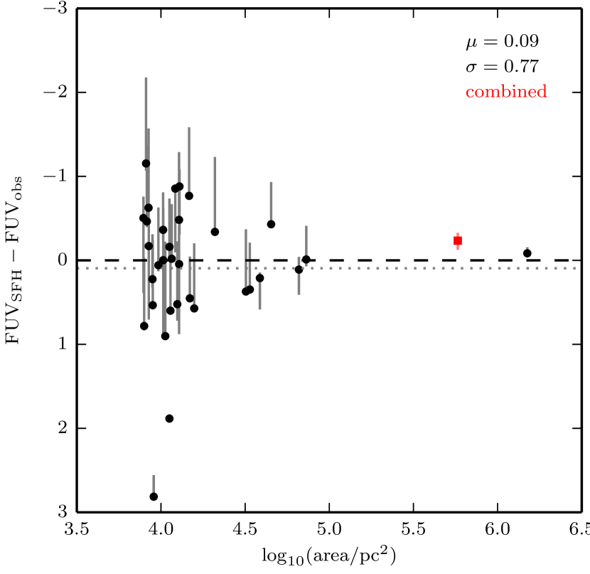
Figure 8.— The difference between the modeled reddened ($\mathrm{FUV_{SFH}}$) and observed ($\mathrm{FUV_{obs}}$, Kang et al., 2009) FUV magnitudes (proportional to the log of the modeled-to-observed flux ratio) versus deprojected area. The dashed line indicates where the magnitudes are equal. On average, the $\mathrm{FUV_{SFH}}$ values are $0.5\,\mathrm{mag}$ fainter than $\mathrm{FUV_{obs}}$ (dotted line) and the $1\sigma$ scatter is $\sim 0.8\,\mathrm{mag}$. The systematic deficiency of the modeled magnitudes is likely due to overestimates in the FUV extinction. The scatter is greatest among the smallest regions and indicates that discrete sampling of the IMF is important on these scales. The combined region from Figure 3, indicated by the red square, shows much better agreement between $\mathrm{FUV_{SFH}}$ and $\mathrm{FUV_{obs}}$ than the individual regions it comprises.

5. SFR estimates

The usual procedure for converting FUV flux into a SFR is to correct the observed flux for extinction, calculate the luminosity, and then apply the proper calibration. To test this method, we derived FUV extinction corrections, $A_{\mathrm{FUV}}$, from the differences between $\mathrm{FUV_{SFH}}$ and $\mathrm{FUV_{SFH,0}}$. The uncertainties in $A_{\mathrm{FUV}}$ were calculated as described in §3.4. The resulting values, listed in Table 3, were used to correct $\mathrm{FUV_{obs}}$.

The extinction-corrected observed FUV magnitudes were converted into SFRs, $\mathrm{SFR_{FUV}}$, using the flux calibration from Kennicutt (1998) with updated coefficients by Hao et al. (2011) and Murphy et al. (2011) (see Kennicutt & Evans, 2012):

$$\left(\frac{\mathrm{SFR_{FUV}}}{M_{\odot}\,\mathrm{yr^{-1}}}\right)=10^{-43.35}\,\left(\frac{L_{\mathrm{FUV}}}{\mathrm{erg\,s^{-1}}}\right)$$ (1)

where $L_{\mathrm{FUV}}$ is the FUV luminosity in $\mathrm{erg\,s^{-1}}$. This calibration was derived using the stellar population synthesis code Starburst99 (Leitherer et al., 1999) assuming that the SFR has been constant over the last $100\,\mathrm{Myr}$. It also assumes a fully populated Kroupa IMF (Kroupa, 2001) and solar metallicity.

The total uncertainties are the quadrature sum of the photometric uncertainties propagated from $\mathrm{FUV_{obs}}$ and the random and systematic uncertainties derived according to §3.4 (where $\mathrm{SFR_{FUV}}$ was calculated for each value of $A_{\mathrm{FUV}}$ from the HMC and $1\sigma$ SFHs). The $\mathrm{SFR_{FUV}}$ values are listed in Table 4 and are shown against the SFHs in Figure 5. Although more sophisticated tracers exist for calculating SFRs (e.g., hybrid tracers discussed in Leroy et al., 2012), none of them can be used with GALEX FUV and NUV data alone and such calculations are therefore outside the scope of this study.

To compare with the flux-based SFRs, we calculated the mean SFR over the last $100\,\mathrm{Myr}$ of the SFH, $\langle\mathrm{SFR}\rangle_{100}=M_{100}\times 10^{-8}\,\mathrm{yr}^{-1}$, where $M_{100}$ is the total mass formed over the same time period. The $\langle\mathrm{SFR}\rangle_{100}$ values are shown in Figure 5, and both $M_{100}$ and $\langle\mathrm{SFR}\rangle_{100}$ are listed in Table 2. The uncertainties were derived as described in §3.4. We also calculated the mean SFR over the last $500\,\mathrm{Myr}$, $\langle\mathrm{SFR}\rangle_{500}$ (Figure 5). The $500\,\mathrm{Myr}$ timescale (the practical age limit of the SFHs, §3.3) is useful for understanding the overall behavior of the regions and illustrates the significance of the SF activity in the last $100\,\mathrm{Myr}$ with respect to the broader history. Figure 9 shows the log ratio of $\mathrm{SFR_{FUV}}$ to $\langle\mathrm{SFR}\rangle_{100}$ versus deprojected region area, and is discussed in §6.2.

Table 4SFRs, ages, and masses from FUV and NUV fluxes.

ID	$\mathrm{SFR_{FUV,0}}\tablenotemark{a}$	$\mathrm{SFR_{FUV}}\tablenotemark{b}$	$\mathrm{Age_{SSP}}\tablenotemark{c}$	$M_{\mathrm{SSP}}\tablenotemark{c}$
	$(\times 10^{-5}\,M_{\odot}\,\mathrm{yr}^{-1})$	$(\times 10^{-5}\,M_{\odot}\,\mathrm{yr}^{-1})$	(Myr)	$(\times 10^{3}\,M_{\odot})$
4285*	$\phantom{0}\phantom{0}2.4\begin{subarray}{c}+0.0\phantom{0}\\ -0.4\phantom{0}\end{subarray}$	$\phantom{0}\phantom{0}13.3\begin{subarray}{c}+0.2\\ -2.6\end{subarray}$	$161.6\begin{subarray}{c}+8.9\phantom{0}\\ -8.9\phantom{0}\end{subarray}$	$\phantom{0}160.00\begin{subarray}{c}+0.00\phantom{0}\phantom{0}\\ -0.00\phantom{0}\phantom{0}\end{subarray}$
4288*	$\phantom{0}\phantom{0}3.2\begin{subarray}{c}+1.4\phantom{0}\\ -0.5\phantom{0}\end{subarray}$	$\phantom{0}\phantom{0}\phantom{0}2.3\begin{subarray}{c}+0.1\\ -0.1\end{subarray}$	$\phantom{0}83.3\begin{subarray}{c}+10.2\\ -9.3\phantom{0}\end{subarray}$	$\phantom{0}\phantom{0}14.00\begin{subarray}{c}+3.00\phantom{0}\phantom{0}\\ -2.00\phantom{0}\phantom{0}\end{subarray}$
4290*	$\phantom{0}33.5\begin{subarray}{c}+1.1\phantom{0}\\ -11.5\end{subarray}$	$\phantom{0}\phantom{0}40.7\begin{subarray}{c}+1.1\\ -4.2\end{subarray}$	$203.9\begin{subarray}{c}+4.0\phantom{0}\\ -4.0\phantom{0}\end{subarray}$	$2000.00\begin{subarray}{c}+0.00\phantom{0}\phantom{0}\\ -0.00\phantom{0}\phantom{0}\end{subarray}$
4292*	$\phantom{0}\phantom{0}5.5\begin{subarray}{c}+7.7\phantom{0}\\ -1.4\phantom{0}\end{subarray}$	$\phantom{0}\phantom{0}\phantom{0}3.1\begin{subarray}{c}+0.2\\ -0.5\end{subarray}$	$\phantom{0}\phantom{0}3.1\begin{subarray}{c}+2.6\phantom{0}\\ -1.5\phantom{0}\end{subarray}$	$\phantom{0}\phantom{0}\phantom{0}1.30\begin{subarray}{c}+1.70\phantom{0}\phantom{0}\\ \phantom{.}\phantom{0}\end{subarray}$
4293*	$\phantom{0}16.0\begin{subarray}{c}+9.8\phantom{0}\\ -0.7\phantom{0}\end{subarray}$	$\phantom{0}\phantom{0}10.8\begin{subarray}{c}+0.9\\ -0.5\end{subarray}$	$169.5\begin{subarray}{c}+8.4\phantom{0}\\ -8.4\phantom{0}\end{subarray}$	$\phantom{0}900.00\begin{subarray}{c}+0.00\phantom{0}\phantom{0}\\ -0.00\phantom{0}\phantom{0}\end{subarray}$
4298*	$\phantom{0}21.6\begin{subarray}{c}+12.9\\ -0.4\phantom{0}\end{subarray}$	$\phantom{0}\phantom{0}29.8\begin{subarray}{c}+0.9\\ -3.7\end{subarray}$	$122.7\begin{subarray}{c}+7.0\phantom{0}\\ -7.0\phantom{0}\end{subarray}$	$\phantom{0}150.00\begin{subarray}{c}+0.00\phantom{0}\phantom{0}\\ -0.00\phantom{0}\phantom{0}\end{subarray}$
4299*	$\phantom{0}\phantom{0}3.4\begin{subarray}{c}+4.4\phantom{0}\\ -0.0\phantom{0}\end{subarray}$	$\phantom{0}\phantom{0}\phantom{0}2.5\begin{subarray}{c}+0.1\\ -0.1\end{subarray}$	$\phantom{0}61.1\begin{subarray}{c}+12.6\\ -12.9\end{subarray}$	$\phantom{0}\phantom{0}12.00\begin{subarray}{c}+3.00\phantom{0}\phantom{0}\\ -2.20\phantom{0}\phantom{0}\end{subarray}$
4308*	$1129.2\begin{subarray}{c}+80.5\\ -37.5\end{subarray}$	$1045.1\begin{subarray}{c}+1.9\\ -2.1\end{subarray}$	$\phantom{0}79.0\begin{subarray}{c}+0.8\phantom{0}\\ -0.7\phantom{0}\end{subarray}$	$9800.00\begin{subarray}{c}+0.00\phantom{0}\phantom{0}\\ -0.00\phantom{0}\phantom{0}\end{subarray}$
4310*	$\phantom{0}\phantom{0}3.1\begin{subarray}{c}+4.1\phantom{0}\\ -0.3\phantom{0}\end{subarray}$	$\phantom{0}\phantom{0}\phantom{0}2.0\begin{subarray}{c}+0.2\\ -0.1\end{subarray}$	$150.5\begin{subarray}{c}+14.2\\ -14.3\end{subarray}$	$\phantom{0}\phantom{0}77.00\begin{subarray}{c}+0.00\phantom{0}\phantom{0}\\ -51.00\phantom{0}\end{subarray}$
4313*	$\phantom{0}\phantom{0}2.9\begin{subarray}{c}+2.6\phantom{0}\\ -1.9\phantom{0}\end{subarray}$	$\phantom{0}\phantom{0}\phantom{0}2.9\begin{subarray}{c}+0.6\\ -0.7\end{subarray}$	$141.2\begin{subarray}{c}+11.7\\ -11.6\end{subarray}$	$\phantom{0}\phantom{0}48.00\begin{subarray}{c}+102.00\\ -0.00\phantom{0}\phantom{0}\end{subarray}$
4314*	$\phantom{0}34.6\begin{subarray}{c}+1.3\phantom{0}\\ -17.6\end{subarray}$	$\phantom{0}\phantom{0}15.8\begin{subarray}{c}+1.7\\ -1.6\end{subarray}$	$\phantom{0}27.5\begin{subarray}{c}+13.0\\ -8.5\phantom{0}\end{subarray}$	$\phantom{0}\phantom{0}64.00\begin{subarray}{c}+21.00\phantom{0}\\ -26.00\phantom{0}\end{subarray}$
4317*	$\phantom{0}\phantom{0}4.2\begin{subarray}{c}+1.0\phantom{0}\\ -2.4\phantom{0}\end{subarray}$	$\phantom{0}\phantom{0}\phantom{0}2.6\begin{subarray}{c}+0.7\\ -0.2\end{subarray}$	$121.8\begin{subarray}{c}+15.5\\ -15.5\end{subarray}$	$\phantom{0}\phantom{0}40.00\begin{subarray}{c}+0.00\phantom{0}\phantom{0}\\ -0.00\phantom{0}\phantom{0}\end{subarray}$
4318*	$\phantom{0}\phantom{0}4.8\begin{subarray}{c}+1.5\phantom{0}\\ -0.6\phantom{0}\end{subarray}$	$\phantom{0}\phantom{0}\phantom{0}7.8\begin{subarray}{c}+1.4\\ -1.1\end{subarray}$	$\phantom{0}18.4\begin{subarray}{c}+11.2\\ -6.7\phantom{0}\end{subarray}$	$\phantom{0}\phantom{0}\phantom{0}1.60\begin{subarray}{c}+1.20\phantom{0}\phantom{0}\\ -0.91\phantom{0}\phantom{0}\end{subarray}$
4320*	$\phantom{0}\phantom{0}5.9\begin{subarray}{c}+3.2\phantom{0}\\ -0.3\phantom{0}\end{subarray}$	$\phantom{0}\phantom{0}\phantom{0}8.9\begin{subarray}{c}+0.5\\ -0.2\end{subarray}$	$\phantom{0}84.7\begin{subarray}{c}+5.4\phantom{0}\\ -5.4\phantom{0}\end{subarray}$	$\phantom{0}180.00\begin{subarray}{c}+20.00\phantom{0}\\ -0.00\phantom{0}\phantom{0}\end{subarray}$
4321*	$\phantom{0}\phantom{0}4.0\begin{subarray}{c}+4.4\phantom{0}\\ -0.0\phantom{0}\end{subarray}$	$\phantom{0}\phantom{0}\phantom{0}2.6\begin{subarray}{c}+0.1\\ -0.1\end{subarray}$	$\phantom{0}66.2\begin{subarray}{c}+14.2\\ -16.8\end{subarray}$	$\phantom{0}\phantom{0}19.00\begin{subarray}{c}+3.00\phantom{0}\phantom{0}\\ -7.00\phantom{0}\phantom{0}\end{subarray}$
4322*	$\phantom{0}\phantom{0}2.5\begin{subarray}{c}+3.8\phantom{0}\\ -0.1\phantom{0}\end{subarray}$	$\phantom{0}\phantom{0}\phantom{0}0.9\begin{subarray}{c}+0.1\\ -0.1\end{subarray}$	$\phantom{0}\phantom{0}5.6\begin{subarray}{c}+7.8\phantom{0}\\ -3.5\phantom{0}\end{subarray}$	$\phantom{0}\phantom{0}\phantom{0}0.24\begin{subarray}{c}+0.32\phantom{0}\phantom{0}\\ -0.12\phantom{0}\phantom{0}\end{subarray}$
4330*	$\phantom{0}\phantom{0}4.2\begin{subarray}{c}+4.8\phantom{0}\\ -0.2\phantom{0}\end{subarray}$	$\phantom{0}\phantom{0}\phantom{0}2.1\begin{subarray}{c}+0.1\\ -0.1\end{subarray}$	$\phantom{0}43.4\begin{subarray}{c}+11.7\\ -14.7\end{subarray}$	$\phantom{0}\phantom{0}23.00\begin{subarray}{c}+16.00\phantom{0}\\ -6.00\phantom{0}\phantom{0}\end{subarray}$
4331	$\phantom{0}\phantom{0}1.0\begin{subarray}{c}+0.8\phantom{0}\\ -0.1\phantom{0}\end{subarray}$	$\phantom{0}\phantom{0}13.3\begin{subarray}{c}+5.5\\ -1.7\end{subarray}$	$130.9\begin{subarray}{c}+8.0\phantom{0}\\ -8.1\phantom{0}\end{subarray}$	$2000.00\begin{subarray}{c}+0.00\phantom{0}\phantom{0}\\ -0.00\phantom{0}\phantom{0}\end{subarray}$
4333	$\phantom{0}\phantom{0}1.3\begin{subarray}{c}+1.3\phantom{0}\\ -0.3\phantom{0}\end{subarray}$	$\phantom{0}\phantom{0}\phantom{0}2.1\begin{subarray}{c}+0.3\\ -0.1\end{subarray}$	$\phantom{0}\phantom{0}1.9\begin{subarray}{c}+0.5\phantom{0}\\ -0.4\phantom{0}\end{subarray}$	$\phantom{0}\phantom{0}\phantom{0}0.40\begin{subarray}{c}+0.00\phantom{0}\phantom{0}\\ -0.00\phantom{0}\phantom{0}\end{subarray}$
4335*	$\phantom{0}\phantom{0}3.7\begin{subarray}{c}+3.8\phantom{0}\\ -0.0\phantom{0}\end{subarray}$	$\phantom{0}\phantom{0}\phantom{0}5.2\begin{subarray}{c}+0.7\\ -0.1\end{subarray}$	$\phantom{0}36.8\begin{subarray}{c}+5.4\phantom{0}\\ -7.4\phantom{0}\end{subarray}$	$\phantom{0}\phantom{0}46.00\begin{subarray}{c}+0.00\phantom{0}\phantom{0}\\ -12.00\phantom{0}\end{subarray}$
4337*	$\phantom{0}20.9\begin{subarray}{c}+1.9\phantom{0}\\ -1.2\phantom{0}\end{subarray}$	$\phantom{0}\phantom{0}20.6\begin{subarray}{c}+2.4\\ -1.1\end{subarray}$	$\phantom{0}13.9\begin{subarray}{c}+4.2\phantom{0}\\ -4.0\phantom{0}\end{subarray}$	$\phantom{0}\phantom{0}16.00\begin{subarray}{c}+22.00\phantom{0}\\ -0.00\phantom{0}\phantom{0}\end{subarray}$
4339*	$\phantom{0}28.9\begin{subarray}{c}+3.0\phantom{0}\\ -8.5\phantom{0}\end{subarray}$	$\phantom{0}\phantom{0}31.9\begin{subarray}{c}+0.2\\ -1.3\end{subarray}$	$\phantom{0}63.5\begin{subarray}{c}+3.1\phantom{0}\\ -3.1\phantom{0}\end{subarray}$	$\phantom{0}\phantom{0}96.00\begin{subarray}{c}+24.00\phantom{0}\\ -0.00\phantom{0}\phantom{0}\end{subarray}$
4345	$\phantom{0}\phantom{0}4.0\begin{subarray}{c}+4.3\phantom{0}\\ -0.3\phantom{0}\end{subarray}$	$\phantom{0}\phantom{0}\phantom{0}6.7\begin{subarray}{c}+1.2\\ -0.4\end{subarray}$	$\phantom{0}\phantom{0}5.5\begin{subarray}{c}+1.3\phantom{0}\\ -1.2\phantom{0}\end{subarray}$	$\phantom{0}\phantom{0}\phantom{0}0.46\begin{subarray}{c}+0.28\phantom{0}\phantom{0}\\ -0.12\phantom{0}\phantom{0}\end{subarray}$
4346*	$\phantom{0}36.5\begin{subarray}{c}+16.4\\ -3.8\phantom{0}\end{subarray}$	$\phantom{0}\phantom{0}36.1\begin{subarray}{c}+0.3\\ -1.3\end{subarray}$	$\phantom{0}18.3\begin{subarray}{c}+1.6\phantom{0}\\ -1.7\phantom{0}\end{subarray}$	$\phantom{0}110.00\begin{subarray}{c}+0.00\phantom{0}\phantom{0}\\ -0.00\phantom{0}\phantom{0}\end{subarray}$
4348*	$\phantom{0}\phantom{0}3.1\begin{subarray}{c}+3.2\phantom{0}\\ -0.1\phantom{0}\end{subarray}$	$\phantom{0}\phantom{0}\phantom{0}5.3\begin{subarray}{c}+0.3\\ -0.3\end{subarray}$	$\phantom{0}\phantom{0}9.3\begin{subarray}{c}+2.9\phantom{0}\\ -1.9\phantom{0}\end{subarray}$	$\phantom{0}\phantom{0}\phantom{0}0.76\begin{subarray}{c}+0.10\phantom{0}\phantom{0}\\ -0.25\phantom{0}\phantom{0}\end{subarray}$
4349*	$\phantom{0}21.6\begin{subarray}{c}+8.1\phantom{0}\\ -8.9\phantom{0}\end{subarray}$	$\phantom{0}\phantom{0}\phantom{0}9.6\begin{subarray}{c}+1.4\\ -0.4\end{subarray}$	$\phantom{0}80.6\begin{subarray}{c}+9.6\phantom{0}\\ -9.2\phantom{0}\end{subarray}$	$\phantom{0}190.00\begin{subarray}{c}+40.00\phantom{0}\\ -30.00\phantom{0}\end{subarray}$
4350*	$\phantom{0}\phantom{0}6.6\begin{subarray}{c}+4.9\phantom{0}\\ -1.0\phantom{0}\end{subarray}$	$\phantom{0}\phantom{0}\phantom{0}5.7\begin{subarray}{c}+0.8\\ -0.3\end{subarray}$	$\phantom{0}41.4\begin{subarray}{c}+6.9\phantom{0}\\ -12.4\end{subarray}$	$\phantom{0}\phantom{0}23.00\begin{subarray}{c}+9.00\phantom{0}\phantom{0}\\ -6.00\phantom{0}\phantom{0}\end{subarray}$
4353*	$\phantom{0}\phantom{0}6.5\begin{subarray}{c}+3.5\phantom{0}\\ -4.3\phantom{0}\end{subarray}$	$\phantom{0}\phantom{0}\phantom{0}5.5\begin{subarray}{c}+1.9\\ -1.0\end{subarray}$	$\phantom{0}\phantom{0}2.3\begin{subarray}{c}+1.9\phantom{0}\\ -0.8\phantom{0}\end{subarray}$	$\phantom{0}\phantom{0}\phantom{0}0.21\begin{subarray}{c}+0.05\phantom{0}\phantom{0}\\ \phantom{.}\phantom{0}\end{subarray}$
4354*	$\phantom{0}\phantom{0}2.7\begin{subarray}{c}+1.3\phantom{0}\\ -0.5\phantom{0}\end{subarray}$	$\phantom{0}\phantom{0}\phantom{0}3.3\begin{subarray}{c}+0.0\\ -0.0\end{subarray}$	$\phantom{0}45.9\begin{subarray}{c}+3.8\phantom{0}\\ -3.8\phantom{0}\end{subarray}$	$\phantom{0}\phantom{0}17.00\begin{subarray}{c}+0.00\phantom{0}\phantom{0}\\ -4.00\phantom{0}\phantom{0}\end{subarray}$
4355	$\phantom{0}\phantom{0}4.8\begin{subarray}{c}+5.8\phantom{0}\\ -0.4\phantom{0}\end{subarray}$	$\phantom{0}\phantom{0}10.0\begin{subarray}{c}+1.9\\ -0.9\end{subarray}$	$\phantom{0}\phantom{0}1.1\begin{subarray}{c}+0.3\phantom{0}\\ \phantom{.}\phantom{0}\end{subarray}$	$\phantom{0}\phantom{0}\phantom{0}1.90\begin{subarray}{c}+0.00\phantom{0}\phantom{0}\\ \phantom{.}\phantom{0}\end{subarray}$
4360	$\phantom{0}\phantom{0}5.2\begin{subarray}{c}+3.2\phantom{0}\\ -3.7\phantom{0}\end{subarray}$	$\phantom{0}\phantom{0}\phantom{0}5.4\begin{subarray}{c}+0.5\\ -0.9\end{subarray}$	$\phantom{0}\phantom{0}2.2\begin{subarray}{c}+0.8\phantom{0}\\ -0.4\phantom{0}\end{subarray}$	$\phantom{0}\phantom{0}\phantom{0}0.28\begin{subarray}{c}\phantom{.}\phantom{0}\\ -0.00\phantom{0}\phantom{0}\end{subarray}$
4362	$\phantom{0}\phantom{0}1.7\begin{subarray}{c}+2.9\phantom{0}\\ -0.0\phantom{0}\end{subarray}$	$\phantom{0}\phantom{0}\phantom{0}3.9\begin{subarray}{c}+0.6\\ -0.1\end{subarray}$	$\phantom{0}29.5\begin{subarray}{c}+11.6\\ -8.3\phantom{0}\end{subarray}$	$\phantom{0}\phantom{0}\phantom{0}5.80\begin{subarray}{c}+2.00\phantom{0}\phantom{0}\\ -2.30\phantom{0}\phantom{0}\end{subarray}$
4364*	$\phantom{0}\phantom{0}1.5\begin{subarray}{c}+1.3\phantom{0}\\ -0.2\phantom{0}\end{subarray}$	$\phantom{0}\phantom{0}\phantom{0}1.5\begin{subarray}{c}+0.0\\ -0.1\end{subarray}$	$\phantom{0}76.1\begin{subarray}{c}+9.6\phantom{0}\\ -9.8\phantom{0}\end{subarray}$	$\phantom{0}\phantom{0}\phantom{0}9.80\begin{subarray}{c}+2.20\phantom{0}\phantom{0}\\ -1.50\phantom{0}\phantom{0}\end{subarray}$
comb.	$368.8\begin{subarray}{c}+31.8\\ -36.4\end{subarray}$	$\phantom{0}297.3\begin{subarray}{c}+0.9\\ -0.9\end{subarray}$

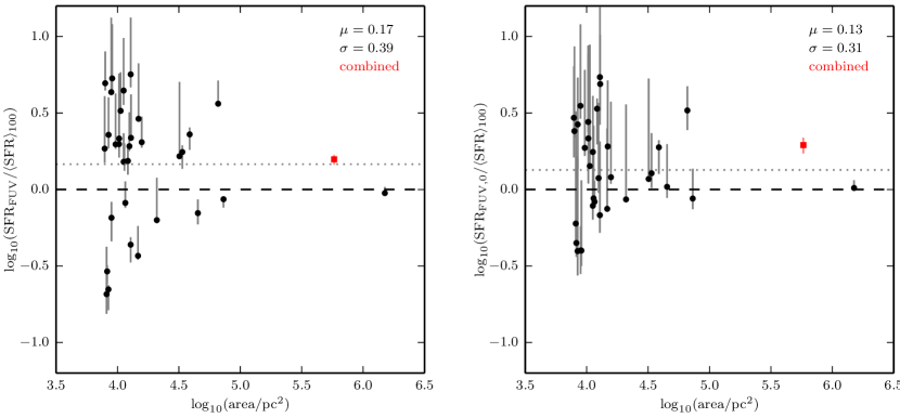
Figure 9.— The log ratio of the FUV flux-based SFRs to the $100\,\mathrm{Myr}$ mean SFR of the SFHs ($\langle\mathrm{SFR}\rangle_{100}$) versus deprojected region area. In the left panel, the flux-based SFRs ($\mathrm{SFR_{FUV}}$) were derived from the extinction-corrected observed FUV magnitudes, and the flux-based SFRs in the right panel ($\mathrm{SFR_{FUV,0}}$) were derived from the intrinsic FUV magnitudes modeled from the SFHs. The dashed lines indicate where the SFRs are equal, and the mean and standard deviation of each log ratio is shown in its respective panel. The systematic overestimation of $\mathrm{SFR_{FUV}}$ in the left panel is likely due to overestimates in the FUV extinction, and the primary sources of the scatter are discrete sampling of the IMF and variability in the SFHs. The mean offset and the scatter are reduced for $\mathrm{SFR_{FUV,0}}$ in the right panel, where the remaining scatter is primarily due to SFH variability. In both panels, the combined region from Figure 3, indicated by the red square, shows much better agreement between the flux-based and mean SFRs than the individual regions it comprises.

6. Discussion

6.1. FUV magnitudes

The differences between the reddened FUV magnitudes modeled from the SFHs and the observed FUV magnitudes of the regions, $\mathrm{FUV_{SFH}-FUV_{obs}}$, shown in Figure 8 are normally distributed with a mean and standard deviation of $\mu=0.09\,\mathrm{mag}$ and $\sigma=0.8\,\mathrm{mag}$, respectively. The $\mathrm{FUV_{SFH}}$ values are consistent with the $\mathrm{FUV_{obs}}$ values on average, demonstrating that the FUV magnitudes are largely free of several potential systematic effects, such as scattering of FUV photons from or into the regions or misinterpretation of the CMDs by MATCH.

The consistency of $\mu$ with zero supports the hypothesis from §3.2 that the $A_{\mathrm{V},f},dA_{\mathrm{V}}$ extinction model adequately describes the dust affecting the MS stars in the regions. Because $A_{\mathrm{FUV}}$ is derived by extrapolating $A_{\mathrm{V},f}$ and $dA_{\mathrm{V}}$ along an extinction curve, the lack of a significant offset between $\mathrm{FUV_{SFH}}$ and $\mathrm{FUV_{obs}}$ justifies our adoption of the average Galactic extinction curve from Cardelli et al. (1989) with the standard value of $R_{\mathrm{V}}=3.1$. This is consistent with results from Barmby et al. (2000) and Bianchi et al. (1996), who found that the overall extinction curves of M31 and the Galaxy are similar for optical and UV wavelengths, respectively.

It is somewhat surprising that assuming the Cardelli et al. (1989) extinction curve does not produce a larger systematic offset between $\mathrm{FUV_{SFH}}$ and $\mathrm{FUV_{obs}}$. Previous studies have shown that local dust properties and the shape of the extinction curve strongly depend on environment (Fitzpatrick & Massa, 2007; Bianchi, 2011; Efremova et al., 2011), which brings into question the applicability of any galaxy-averaged extinction curve to specific locations within a galaxy. Furthermore, results from Bianchi (2011) and Efremova et al. (2011) indicate that areas of intense SF, such as UV-bright regions, tend to have extinction curves that are steeper in the UV regime. Despite these details, we find that, given a mean visual extinction of $A_{\mathrm{V},f}+dA_{\mathrm{V}}\approx 1.5$, the $\mu=0.09\,\mathrm{mag}$ offset is consistent with a value of $R_{\mathrm{V}}$ between 3.1 and 3.2. This is well within the range of $R_{\mathrm{V}}$ values obtained by Fitzpatrick & Massa (2007) for 328 lines of sight in the Galaxy, for which the mean and standard deviation was 3.0 and 0.3, respectively.

Although the modeled and the observed FUV magnitudes agree on average, Figure 8 shows that the scatter in $\mathrm{FUV_{SFH}-FUV_{obs}}$ about the mean is larger than the uncertainties. A possible source of this scatter is the assumption of a homogeneous metallicity for the modeled FUV magnitudes, $[\mathrm{M/H}]=-0.3\,\mathrm{dex}$, whereas the actual final metallicity values for most of the regions varied between $[\mathrm{M/H}]=-0.6$ and $0.0\,\mathrm{dex}$ (§3.3). Figure 6 in Johnson et al. (2013) shows how the FUV luminosity of a constant SFR model changes as a function of input metallicity. Near $[\mathrm{M/H}]=-0.3\,\mathrm{dex}$ ($\log_{10}(Z/Z_{\odot})\approx-0.3$, assuming the helium-to-metals enrichment law from Bressan et al., 2012), changing $[\mathrm{M/H}]$ by $\pm 0.1\,\mathrm{dex}$ causes the modeled FUV flux to change by $\mp 0.015\,\mathrm{dex}$, or $\pm 0.038\,\mathrm{mag}$ in terms of FUV magnitudes. Given a metallicity dispersion of $0.3\,\mathrm{dex}$, variations from the assumed metallicity therefore lead to an uncertainty of about $0.1\,\mathrm{mag}$ in $\mathrm{FUV_{SFH}}$. The effect of assuming a homogeneous metallicity contributes only a small amount to the total scatter.

Figure 8 shows that the scatter in $\mathrm{FUV_{SFH}-FUV_{obs}}$ appears to increase with decreasing region area. Because the regions are all defined to have the same minimum FUV surface brightness, the masses of the regions roughly scale with area, implying that the scatter is greatest for the regions with the lowest masses. A well-known characteristic of low-mass systems is that the distribution of stellar masses is noticeably discrete, particularly with respect to the high-mass end of the IMF where the relative probability of star formation is low. As a result, the sampling of stellar masses from the IMF is not as complete in such systems as for higher-mass systems. This is illustrated in the CMDs in Figure 3, which show the upper MS in many of the regions to be sparsely populated compared with the much larger region 4308.

To model UV fluxes from the SFHs, FSPS assumes that the stellar mass formed in each age bin represents a full sampling of the IMF, which is inconsistent with the actual sampling of stellar masses in the regions. Therefore, the modeled flux is underestimated in regions that have an apparent excess of massive MS stars relative to the number expected from a fully populated IMF, and is overestimated in regions with an apparent lack of massive MS stars. The size of this discrepancy should be larger for regions with lower masses due to the sampling of the IMF becoming more discrete. Given that area is a proxy for mass in our sample, the scatter in Figure 8 is indeed consistent with this expectation. We therefore consider the scatter in the magnitudes to be caused by the application of the full-IMF assumption where the effect of discrete sampling is important.

To further test the impact of region size on the magnitude discrepancy, we constructed a larger effective region by combining the photometry of all regions, excluding region 4308 (the largest region). We then measured the SFH and modeled the total FUV magnitude following the same procedure used for the other regions. The total area and effective observed FUV magnitude (from the combination of the observed magnitudes of the individual regions) are given in Table 1, and the CMD is shown in Figure 3. We show the SFH and the corresponding best-fit extinction parameters in Figure 5 and Table 2, respectively. The modeled FUV magnitude is listed in Table 3.

The combined region in Figure 8 has a magnitude difference similar to region 4308 and is more consistent with the sample mean than the majority of the individual regions it comprises. The combined region apparently produces a much better representation of stellar masses in the IMF than when the regions are considered individually, making the combined region more consistent with the full-IMF assumption. This result supports our hypothesis that the scatter in the magnitudes is largely explained as a sampling effect of the IMF.

We estimate that discrete sampling becomes important for the UV-bright regions below an area of $\sim 10^{5}\,\mathrm{pc^{2}}$, and amounts to an uncertainty of $\sigma=0.8\,\mathrm{mag}$ in the modeled FUV magnitudes, or a factor of $10^{|\sigma/-2.5|}=2$ in flux. Determining a characteristic area threshold from our sample is difficult, however, due to the lack of regions with areas between $10^{5}$ and $10^{6}\,\mathrm{pc^{2}}$.

6.2. SFR estimates from FUV flux

Figure 9 shows many of the same features as Figure 8, namely log-normally distributed ratios with a mean offset and scatter that is largest among the smallest regions (see §6.1). The log-normal distribution for the $\mathrm{SFR_{FUV}/\langle SFR\rangle_{100}}$ values shown in Figure 9 has $\mu=0.2$ and $\sigma=0.4$.

The offset in Figure 9 is less than the scatter. The FUV-based SFRs are therefore consistent with the mean SFRs from the SFHs on average, although the offset is somewhat larger relative to the scatter than in Figure 8. The consistency of the FUV magnitudes in Figure 8 shows that the offset in the SFR ratios is not due to scattering of FUV photons, misinterpretation of the CMDs by MATCH, a deficiency in the extinction model, or an inaccurate extinction curve. Additionally, both $\mathrm{SFR_{FUV}}$ and $\langle\mathrm{SFR}\rangle_{100}$ assume a timescale of $100\,\mathrm{Myr}$, so the offset is also not due to inconsistent timescales.

One difference between $\mathrm{SFR_{FUV}}$ and $\langle\mathrm{SFR}\rangle_{100}$, however, is that the FUV flux calibration was derived assuming solar metallicity. The FUV brightness of a stellar population decreases with increasing metallicity (see §6.1), so the SFR of a high-metallicity population would need to be greater than that of a low-metallicity population with the same FUV flux and SFH. Specifically, overestimating $[\mathrm{M/H}]$ by $0.1\,\mathrm{dex}$ causes the SFR to be overestimated by $0.015\,\mathrm{dex}$.

Because nearly all of the final metallicities were subsolar, the majority of the $\mathrm{SFR_{FUV}}$ values are overestimated to some degree. Solar metallicity is higher than the mean final metallicity from MATCH by $0.3\,\mathrm{dex}$, so the FUV-based SFRs are overestimated by about $0.05\,\mathrm{dex}$ on average. Variations from the metallicity assumed by the flux calibration therefore account for approximately one third of the $\mu=0.2$ offset in Figure 9. With no other obvious systematic effects at work, we attribute the remaining offset to low-number statistics.

Like FSPS, the FUV flux calibration from Kennicutt (1998) assumes that the IMF is fully populated, so discrete sampling of the IMF should produce a similar amount of scatter in Figures 8 and 9. Regions that are brighter for their mass than expected from the full-IMF assumption will have their FUV-based SFRs overestimated, and regions that are fainter than expected will have their SFRs underestimated. As in Figure 8, Figure 9 shows that this discrepancy increases with decreasing area. The scatter in the SFR ratios therefore appears consistent with the application of the full-IMF assumption to low-mass regions. By comparing the $\sigma$ parameters of the log-normal distributions in Figures 8 and 9 ($|0.8/-2.5|=0.3$ and 0.4, respectively), however, we find that the SFR ratios are somewhat more scattered than the magnitude differences. This suggests that there is an additional factor contributing to the scatter.

In addition to the full-IMF assumption, the FUV flux calibration assumes a constant SFR over at least the past $\sim 100\,\mathrm{Myr}$. It is clear from the SFHs in Figure 3 that none of the regions are consistent with this assumption. To test how the inconsistency with the constant-SFR assumption affects the SFR estimates, we used the FUV flux calibration to derive another set of SFRs, $\mathrm{SFR_{FUV,0}}$, from the modeled intrinsic magnitudes in Table 3. Both FSPS and the flux calibration assume a fully populated IMF, so $\mathrm{SFR_{FUV,0}}$ is determined self-consistently. Also, despite the fact that the regions are largely inconsistent with the full-IMF assumption, $\mathrm{\langle SFR\rangle_{100}}$ depends only on the total mass formed in the SFH, not on how the stellar masses were sampled from the IMF. Therefore, any discrepancies between $\mathrm{SFR_{FUV,0}}$ and $\mathrm{\langle SFR\rangle_{100}}$ beyond the measured uncertainties are not due to discrete IMF sampling.

The log ratios of $\mathrm{SFR_{FUV,0}}$ to $\langle\mathrm{SFR}\rangle_{100}$ are shown versus deprojected region area in Figure 9. As for the SFR ratios from the observed FUV magnitudes, we assumed a log-normal distribution and calculated $\mu$ and $\sigma$ to be 0.1 and 0.3, respectively. As expected, we find that the FUV-based SFRs are consistent with the mean SFRs on average. The SFR ratios are widely scattered, indicating that the accuracy of the FUV-based SFR estimates is strongly affected by variations in the SFHs. In the extreme case of an SSP, Leroy et al. (2012) found that FUV-based SFR estimates are intrinsically scattered by a factor of $\sim 3$ to 4 ($\sigma\approx 0.5$ to 0.6 in log space) due to uncertainty about the age of the SSP within a $100\,\mathrm{Myr}$ timescale. The uncertainty we measure, $\sigma=0.3$, is within the intrinsic limit, which we expect given that the regions are more complex than SSPs (see §6.3).

The dependence of the flux-based SFRs on the SFHs is further illustrated by the combined region in Figure 9. The $\mathrm{SFR_{FUV,0}}/\mathrm{\langle SFR\rangle_{100}}$ ratio for the combined region is similar to that of region 4308 (the largest region) and is more consistent with unity than for most of the individual regions it comprises. By combining the regions, many of the variations in the individual SFHs are averaged out and the combined SFH is more constant by comparison.

Taken together, the uncertainties due to discrete sampling of the IMF and variability in the SFHs account for the total amount of scatter in the $\mathrm{SFR_{FUV,0}/\langle SFR\rangle_{100}}$ ratios, as shown from the quadrature sum of the $\sigma$ values of the log-normals, $0.3^{2}+0.3^{2}\approx 0.4^{2}$. The uncertainty components are also the same size, demonstrating that satisfying the full-IMF assumption and satisfying the constant-SFR assumption are equally important for obtaining precise SFR estimates from the FUV flux calibration. Inconsistencies with the full-IMF and constant-SFR assumptions appear to become important in UV-bright regions smaller than $\sim 10^{5}\,\mathrm{pc^{2}}$. Assuming that one has a robust FUV extinction correction), FUV-based SFRs estimated for regions smaller than this limit are uncertain by a factor of about 2.5. We stress that this factor represents the best case uncertainty, as the dust corrections for integrated UV flux are often unclear and substantial. Our results are consistent with warnings from Murphy et al. (2011), Kennicutt & Evans (2012), and Leroy et al. (2012) that flux calibrations become problematic on sub-kpc scales.

Perhaps the most important assumptions behind the flux calibration method are the assumed SFH and that SFR has a clear relationship with observed flux. However, it is ambiguous whether the difference in flux between two populations is due to a simple difference in SFR because the observed flux strongly depends on the underlying SFH. This dependence is observed on scales both large and small, e.g., as demonstrated for UV color in spiral galaxies by Barnes et al. (2011) and for FUV flux in our sample of UV-bright regions. We find, for example, that although region 4299 and 4350 have total masses (and thus mean SFRs) within 5%, their SFHs are quite different and the FUV flux of region 4350 is more than a factor of 2 brighter than that of 4299. We also find that FUV flux is often degenerate with SFH (a wide range of SFHs can give rise to the same FUV flux), such as the case for regions 4318 and 4330. These complexities illustrate the inherent difficulty of using integrated flux alone to characterize SF.

6.3. SSP ages and masses

Because the integrated UV spectrum of an SSP evolves significantly over relatively short timescales ($\sim$ few Myr, as indicated in SSP models from Leitherer et al., 1999), the integrated $\mathrm{FUV-NUV}$ color can, in principle, be used to estimate age through population synthesis modeling. Clearly, this technique rests on the assumption that the population approximates an SSP, i.e., that the population can be characterized by a single age. The SSP assumption is typically acceptable for stellar clusters where stars are generally formed at the same epoch, but it becomes untenable whenever the SFH is more complex than a single SF event.

K09 estimated SSP ages, $\mathrm{Age_{SSP}}$, for the regions by comparing the observed $\mathrm{FUV-NUV}$ color with Padova stellar evolution models (Girardi et al., 2010) for a range of metallicities and dust types. The models were reddened according to the average $E(\mathrm{B-V})$ measured in the regions (see §3.2). The ages derived for solar metallicity and $R_{\mathrm{V}}=3.1$ are shown with the SFHs in Figure 5 and are listed in Table 4. It is immediately clear from the SFHs that the majority of the regions to not approximate SSPs and that the very concept of assigning single ages to these regions is invalid. Furthermore, the $\mathrm{Age_{SSP}}$ values often do not correspond to the main episodes of SF.

The corresponding SSP masses, $M_{\mathrm{SSP}}$, were estimated by K09 from $\mathrm{Age_{SSP}}$ and the FUV luminosity. We list the $M_{\mathrm{SSP}}$ values in Table 4 and show the log of $M_{\mathrm{SSP}}/M_{100}$ versus deprojected region area in Figure 10. Most of the $M_{\mathrm{SSP}}$ values are within one to two orders of magnitude of $M_{100}$. This large uncertainty range is a consequence of applying the SSP assumption to regions that are generally not SSPs. By coloring each point in Figure 10 by $\mathrm{Age_{SSP}}$, we find that the masses for regions determined to be young are underestimated, and the masses for regions determined to be older are overestimated (an old SSP must be more massive than a young SSP to have the same UV luminosity). This trend is observed independent of region size.

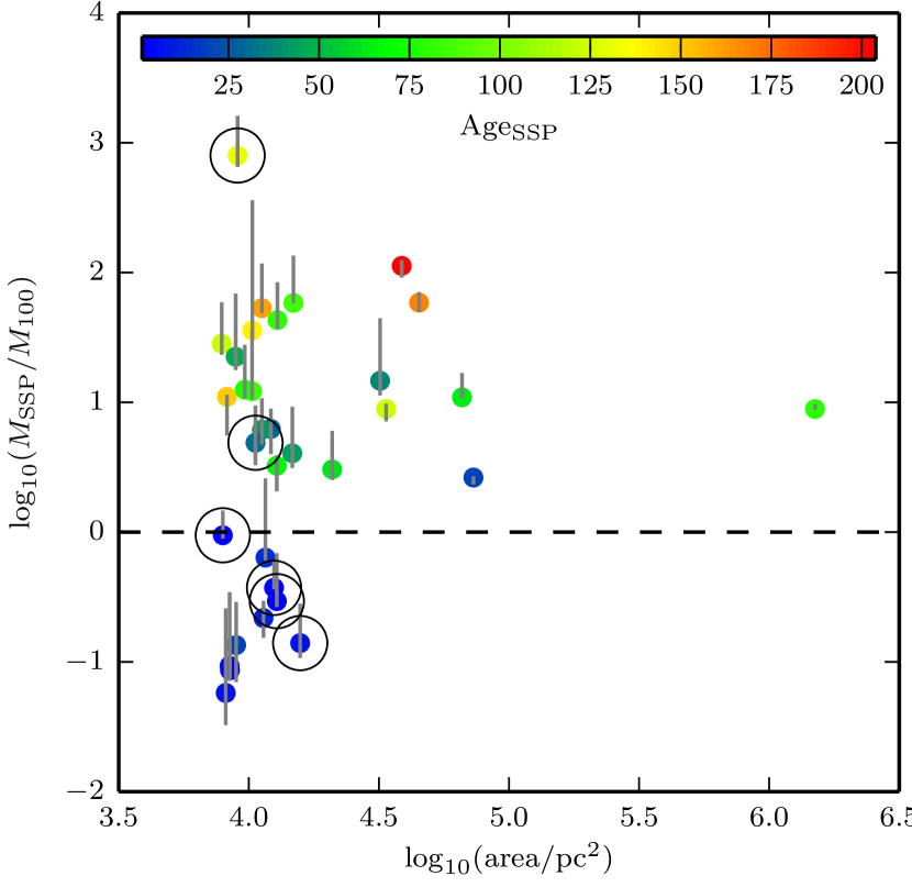
Figure 10.— The log ratio of the SSP masses based on UV color and luminosity ($M_{\mathrm{SSP}}$) to the total mass formed over the last $100\,\mathrm{Myr}$ of the SFHs ($M_{100}$) versus deprojected region area. The markers are colored according to the SSP age, $\mathrm{Age_{SSP}}$, corresponding to $M_{\mathrm{SSP}}$. The dashed line indicates where the masses are equal. SSP masses are underestimated and overestimated for regions that are estimated to be young and old, respectively. The circled points indicate the most SSP-like regions identified in the sample §6.3. At $\log_{10}(M_{\mathrm{SSP}}/M_{100})\approx 3$, region 4331 is extremely discrepant and we do not include it in our SSP analysis. The $M_{\mathrm{SSP}}$ values for the other SSP-like regions indicate a factor of 3 to 4 uncertainty with respect to the $M_{100}$ values.

Although most of the regions are not SSPs, we do find that the SSP assumption is justified in some cases. To identify SSP-like regions, we calculated the ratio of the mass formed in the age bin with the highest SFR over the last $100\,\mathrm{Myr}$, $M_{\mathrm{peak}}$, to the total mass formed over the same time period, $M_{100}$. The values of $M_{\mathrm{peak}}$, $M_{\mathrm{peak}}/M_{100}$, and $\mathrm{Age_{peak}}$ (the mean age of the bin containing $M_{\mathrm{peak}}$) are listed in Table 2. We considered any region with $M_{\mathrm{peak}}/M_{100}\geq 0.9$ to be consistent with an SSP, i.e., any region that has formed more than 90% of its total mass in a single age bin over the last $100\,\mathrm{Myr}$. We found that 18% of the regions (6 of 33; 4331, 4333, 4345, 4355, 4360, and 4362) meet this criterion and we indicate them in Tables 1, 2, 3 and 4.

Except for region 4331, the mean discrepancy between $\mathrm{Age_{SSP}}$ and $\mathrm{Age_{peak}}$ for the SSP-like regions is $10\,\mathrm{Myr}$. On average, $M_{\mathrm{SSP}}$ is consistent with $M_{100}$ to within a factor of 3 or 4 (excluding region 4331). These age and mass discrepancies are often larger than the error bars shown in Figures 5 and 10. Region 4331 is extremely discrepant in both age ($\mathrm{Age_{SSP}-Age_{peak}}=80\,\mathrm{Myr}$) and mass ($M_{\mathrm{SSP}}/M_{100}=800$) for reasons that are unclear, and we do not include it in the remaining analyses.

The uncertainties in $\mathrm{Age_{SSP}}$ are about $3\,\mathrm{Myr}$, on average, and are propagated solely from the photometric uncertainties. We suggest that these uncertainties are underreported, given that metallicity and extinction can potentially introduce systematics that are much larger than the uncertainties in FUV luminosity and $\mathrm{FUV-NUV}$ color. We consider below how metallicity and extinction affect the age and mass estimates.

Metallicity increases the rate at which an SSP becomes redder with age (Bianchi, 2011; Kang et al., 2009). Therefore, if metallicity is overestimated, then $\mathrm{Age_{SSP}}$ will be underestimated. To test how significantly metallicity affects the ages of the SSP-like regions, we compared the ages for solar metal abundance with the ages derived by K09 for $Z=0.05$. The change in metallicity decreased the SSP age estimates by an average of $6\,\mathrm{Myr}$. We also compared the corresponding masses and found that the masses for solar metal abundance were, on average, a factor of 2 larger than the those for $Z=0.05$.

Since UV flux is highly susceptible to dust extinction, any errors in the applied reddening values can significantly affect the derived SSP ages and masses. Namely, if $E(\mathrm{B-V})$ is underestimated, then the corrected $\mathrm{FUV-NUV}$ color will be redder than it should be (assuming the extinction curve of Cardelli et al., 1989, although this is another potential source of uncertainty), causing an overestimate in $\mathrm{Age_{SSP}}$. The change in $M_{\mathrm{SSP}}$ is less clear because underestimating the FUV luminosity and overestimating the age have opposite effects.

To quantify the impact of changes in $\mathrm{FUV-NUV}$ color on $\mathrm{Age_{SSP}}$ and $M_{\mathrm{SSP}}$, we used FSPS (see §4) to model the time evolution of the UV magnitudes of an SSP with solar metallicity. For a $10\,\mathrm{Myr}$ old SSP ($\mathrm{FUV-NUV}\approx-0.09$), we found that a $0.1\,\mathrm{mag}$ reduction in $E(\mathrm{B-V})$ causes the age to be overestimated by $25\,\mathrm{Myr}$ and the mass to be overestimated by a factor of 2.6. $\mathrm{Age_{SSP}}$ and $M_{\mathrm{SSP}}$ are therefore highly sensitive to changes in $\mathrm{FUV-NUV}$.

Systematics from the assumed metallicity and the extinction correction can plausibly account for the observed age and mass discrepancies among the SSP-like regions. From these discrepancies, we propose that more realistic uncertainties for the ages and the masses derived from UV flux are $10\,\mathrm{Myr}$ and a factor of 3 to 4, respectively, though the limited number of regions resembling SSPs makes these uncertainties difficult to determine more precisely. The most striking aspect of this analysis is that over 80% of the regions in the sample are entirely inconsistent with the SSP assumption in the first place, a fact that could not be known without measuring the SFHs, calling into question the practice of deriving ages and masses for populations that are not confirmed SSPs.

7. Conclusion

In this study, we have derived the recent ($<500\,\mathrm{Myr}$) SFHs of 33 UV-bright regions in M31 using optical HST observations from PHAT. The regions were defined by K09 based on GALEX FUV surface brightness and have areas ranging from $8\times 10^{3}$ to $1.5\times 10^{6}\,\mathrm{pc}^{2}$. We used the SFH code MATCH to fit the CMDs of the regions and measure their the SFHs based on the resolved stars from the PHAT photometry. We modeled the extinction in the regions using a foreground parameter and a differential parameter, which were optimized for each region to find the best-fit SFH.

We used FSPS to model both the intrinsic and reddened FUV and NUV magnitudes of the regions based on their SFHs. The differences between the modeled reddened and the observed FUV magnitudes, $\mathrm{FUV_{SFH}-FUV_{obs}}$, followed a normal distribution with $\mu=0.09$ and $\sigma=0.3$. On average, the $\mathrm{FUV_{SFH}}$ values were consistent with the $\mathrm{FUV_{obs}}$ values, confirming the reliability of the SFHs, our extinction model, and the Cardelli et al. (1989) extinction curve. We attribute the scatter in the flux ratios to the assumption made by FSPS that the IMF is fully populated while the actual distribution of stellar masses becomes more discrete as smaller regions are considered.

The observed, extinction-corrected FUV magnitudes were converted into SFRs, $\mathrm{SFR_{FUV}}$, using the FUV flux calibration from Kennicutt (1998) with updated coefficients by Hao et al. (2011) and Murphy et al. (2011). We also derived the mean SFRs for the last $100\,\mathrm{Myr}$ of the SFHs, $\langle\mathrm{SFR}\rangle_{100}$. The $\mathrm{SFR_{FUV}}/\langle\mathrm{SFR}\rangle_{100}$ ratios were log-normally distributed with $\mu=0.2$ and $\sigma=0.4$. Overall, the $\mathrm{SFR_{FUV}}$ values were consistent with the $\langle\mathrm{SFR}\rangle_{100}$ values, though a small amount of the offset was attributable to inconsistencies with the metallicity assumed by the flux calibration.

The intrinsic modeled FUV magnitudes were also converted into SFRs, $\mathrm{SFR_{FUV,0}}$, which were free from biases due to extinction corrections and IMF sampling. The log-normal for the $\mathrm{SFR_{FUV,0}}/\langle\mathrm{SFR}\rangle_{100}$ ratios had $\mu=0.1$ and $\sigma=0.3$, indicating that assuming a constant SFR (implicit in the flux calibration) for regions with highly variable SFHs is an important source of scatter. We conclude that the total scatter in the $\mathrm{SFR_{FUV}}/\langle\mathrm{SFR}\rangle_{100}$ ratio is due to the assumptions of a full IMF and a constant SFR in regions where discrete sampling of the IMF and high variability in the SFHs are important. Combined, these effects result in a factor of 2.5 uncertainty in the FUV-based SFRs. Although there is a significant lack of regions in our sample with areas between $10^{5}$ and $10^{6}\,\mathrm{pc}^{2}$, we estimate that discrete IMF sampling and SFH variability become important below $10^{5}\,\mathrm{pc}^{2}$, or scales of a few hundred pc.

Ages and masses were derived for the regions by K09 from observed $\mathrm{FUV-NUV}$ color and FUV luminosity, using the assumption that the regions are SSPs. By comparing the ages to the SFHs, we found that most of the regions are entirely inconsistent with the SSP assumption. Furthermore, the ages often did not correspond to the main episodes of SF, and the masses were discrepant with the masses integrated from the SFHs by up to 2 orders of magnitude. These results call into question the practice of deriving ages and masses for populations that are not confirmed SSPs.

We identified SSP-like regions as regions which formed 90% or more of their mass over the past $100\,\mathrm{Myr}$ in a single age bin of their SFH. These regions accounted for 18% of our sample (6 of 33). Among this subset, we found discrepancies of $10\,\mathrm{Myr}$ in the ages and a factor of $3-4$ in the masses derived from UV flux, most likely due to systematics in metallicity and extinction. We propose that these discrepancies represent realistic uncertainties in the SSP ages and masses, though the limited number of SSP-like regions in our sample makes the uncertainties difficult to determine. Finally, identification of the SSP-like regions was not possible from integrated FUV flux.

We thank Y. Kang for his assistance in understanding the results presented in Kang et al. (2009). This research has made use of NASA’s Astrophysics Data System Bibliographic Services and the NASA/IPAC Extragalactic Database (NED), which is operated by the Jet Propulsion Laboratory, California Institute of Technology, under contract with the National Aeronautics and Space Administration. This work was supported by the Space Telescope Science Institute through GO-12055. Support for D. R. W is provided by NASA through Hubble Fellowship grant HST-HF-51331.01 awarded by the Space Telescope Science Institute, which is operated by the Association of Universities for Research in Astronomy, Inc., under NASA contract NAS 5-26555. This research made use of Astropy, a community-developed core Python package for Astronomy (Astropy Collaboration et al., 2013), as well as NumPy and SciPy Oliphant (2007), IPython (Pérez & Granger, 2007), and Matplotlib (Hunter, 2007).

References

• Astropy Collaboration et al. (2013) Astropy Collaboration, Robitaille, T. P., Tollerud, E. J., et al. 2013, A&A, 558, A33
• Ballesteros-Paredes et al. (2011) Ballesteros-Paredes, J., Vázquez-Semadeni, E., Gazol, A., et al. 2011, MNRAS, 416, 1436
• Barmby et al. (2000) Barmby, P., Huchra, J. P., Brodie, J. P., et al. 2000, AJ, 119, 727
• Barnes et al. (2011) Barnes, K. L., van Zee, L., & Skillman, E. D. 2011, ApJ, 743, 137
• Berkhuijsen & Fletcher (2008) Berkhuijsen, E. M., & Fletcher, A. 2008, MNRAS, 390, L19
• Bianchi et al. (1996) Bianchi, L., Clayton, G. C., Bohlin, R. C., Hutchings, J. B., & Massey, P. 1996, ApJ, 471, 203
• Bianchi (2011) Bianchi, L. 2011, Ap&SS, 335, 51
• Bressan et al. (2012) Bressan, A., Marigo, P., Girardi, L., et al. 2012, MNRAS, 427, 127
• Cardelli et al. (1989) Cardelli, J. A., Clayton, G. C., & Mathis, J. S. 1989, ApJ, 345, 245
• Conroy et al. (2009) Conroy, C., Gunn, J. E., & White, M. 2009, ApJ, 699, 486
• Conroy & Gunn (2010) Conroy, C., & Gunn, J. E. 2010, ApJ, 712, 833
• Dalcanton et al. (2012) Dalcanton, J. J., Williams, B. F., Lang, D., et al. 2012, ApJS, 200, 18
• Dalcanton et al. (2014) Dalcanton, J. J., Fouesneau, M., Hogg, D. W., et al. 2014, preprint
• Dolphin (2000) Dolphin, A. E. 2000, PASP, 112, 1383
• Dolphin (2002) Dolphin, A. E. 2002, MNRAS, 332, 91
• Dolphin (2013) Dolphin, A. E. 2013, ApJ, 775, 76
• Efremova et al. (2011) Efremova, B. V., Bianchi, L., Thilker, D. A., et al. 2011, ApJ, 730, 88
• Fitzpatrick & Massa (2007) Fitzpatrick, E. L., & Massa, D. 2007, ApJ, 663, 320
• Girardi et al. (2005) Girardi, L., Groenewegen, M. A. T., Hatziminaoglou, E., & da Costa, L. 2005, A&A, 436, 895
• Girardi et al. (2010) Girardi, L., Williams, B. F., Gilbert, K. M., et al. 2010, ApJ, 724, 1030
• Gogarten et al. (2009) Gogarten, S. M., Dalcanton, J. J., Williams, B. F., et al. 2009, ApJ, 691, 115
• Hao et al. (2011) Hao, C.-N., Kennicutt, R. C., Johnson, B. D., et al. 2011, ApJ, 741, 124
• Hill et al. (2008) Hill, A. S., Benjamin, R. A., Kowal, G., et al. 2008, ApJ, 686, 363
• Hunter (2007) Hunter, J. D. 2007, Computing in Science & Engineering, 9, 3
• Johnson et al. (2013) Johnson, B. D., Weisz, D. R., Dalcanton, J. J., et al. 2013, ApJ, 772, 8
• Kang et al. (2009) Kang, Y., Bianchi, L., & Rey, S.-C. 2009, ApJ, 703, 614
• Kennicutt (1998) Kennicutt, R. C., Jr. 1998, ARA&A, 36, 189
• Kennicutt & Evans (2012) Kennicutt, R. C., & Evans, N. J. 2012, ARA&A, 50, 531
• Kroupa (2001) Kroupa, P. 2001, MNRAS, 322, 231
• Leitherer et al. (1999) Leitherer, C., Schaerer, D., Goldader, J. D., et al. 1999, ApJS, 123, 3
• Leroy et al. (2012) Leroy, A. K., Bigiel, F., de Blok, W. J. G., et al. 2012, AJ, 144, 3
• McConnachie et al. (2005) McConnachie, A. W., Irwin, M. J., Ferguson, A. M. N., et al. 2005, MNRAS, 356, 979
• Morrissey et al. (2007) Morrissey, P., Conrow, T., Barlow, T. A., et al. 2007, ApJS, 173, 682
• Murphy et al. (2011) Murphy, E. J., Condon, J. J., Schinnerer, E., et al. 2011, ApJ, 737, 67
• Oliphant (2007) Oliphant, T. E. 2007, Computing in Science & Engineering, 9, 3
• Pérez & Granger (2007) Pérez, F., Granger, B. E. 2007, Computing in Science and Engineering, 9, 3
• Shetty et al. (2011) Shetty, R., Glover, S. C., Dullemond, C. P., & Klessen, R. S. 2011, MNRAS, 412, 1686
• Tully (1994) Tully, R. B. 1994, VizieR Online Data Catalog, 7145, 0