Perspectives of current-layer diagnostics
in solar flares

Abstract

Context. A reconnecting current layer is a ‘heart’ of a solar flare, because it is a place of magnetic-field energy release. However there are no direct observations of these layers.

Aims. The aim of our work is to understand why we actually do not directly observe current layers and what we need to do it in the future.

Methods. The method is based on a simple mathematical model of a super-hot ($T\ga 10^{8}$ K) turbulent-current layer (SHTCL) and a model of plasma heating by the layer.

Results. The models allow us to study a correspondence between the main characteristics of the layer, such as temperature and dimensions, and the observational features, such as differential and integral emission measure of heated plasma, intensity of spectral lines Fe xxvi (1.78 and 1.51 Å) and Ni xxvii (1.59 Å). This method provides a theoretical basis for determining parameters of the current layer from observations.

Conclusions. Observations of SHTCLs are difficult, because the spectral line intensities are faint, but it is theoretically possible in the future. Observations in X-ray range 1.5–1.8 Å with high spectral resolution (better than 0.01 Å) and high temporal resolution (seconds) are needed. It is also very important to interpret the observations using a multi-temperature approach instead of the usual single or double temperature method.

1 Introduction

Solar flares are the brightest events of solar activity. High energy, about $2\times 10^{32}$ ergs, is released during a typical flare; it is expended on heat fluxes, particle acceleration, plasma flows, etc. The basis of this phenomenon is magnetic reconnection, which converts the magnetic-field energy into other forms. The conversion occurs in a reconnecting current layer. It is formed in the place where opposite-directed magnetic fluxes of an active region interact among themselves (e.g., Priest & Forbes 2000; Somov 2006b).

Rich information about solar flares can be obtained from observations in X-rays, which arise due to radiation of high-temperature ($10^{7}-10^{8}$ K) plasma and accelerated (up to MeV energies) electrons. Spacecrafts, such as Hinotori, Yohkoh, Solar Maximum Mission (SMM), and Reuven Ramaty High Energy Solar Spectroscopic Imager (RHESSI), provide indirect evidence of magnetic reconnection in flares: cusp-shaped coronal structures, shrinkage of newly reconnected field lines, reconnection inflows and outflows, a hard X-ray source above the soft X-ray loop top, and others (Emslie et al. 2004; Fletcher et al. 2011; Hudson 2011 and references therein).

Sui & Holman (2003) describe the limb flare on 2002 April 15. The double-source structure was observed by RHESSI in the range of 10–20 keV. The temperature of the lower source, corresponding to flare loops, increased toward higher altitudes, while the temperature of the coronal source increased toward lower altitudes. This is interpreted as a current layer formation between the two sources. We note that the central part of the structure, the super-hot turbulent-current layer (SHTCL), remains empty on the images. A similar pattern was also observed in the flare on 2002 April 30 (Liu et al. 2008). Caspi & Lin (2010) report RHESSI observation of the flare on 2002 July 23. A super-hot elongated source at $\sim 4\times 10^{7}$ K is situated higher and separately from a colder source at $\sim 2\times 10^{7}$ K. It also agrees well with a concept of a current layer located higher in the corona.

The first image of a large-scale reconnecting current layer is presented by Liu et al. (2010). They describe a bright structure of length $>0.25R_{\odot}$ and width $(5-10)\times 10^{8}$ cm, which is situated above the cusp-shaped loop at heights $\sim(0.78-1.05)R_{\odot}$ and associated with a coronal mass ejection (CME). It was observed by extreme ultraviolet imaging telescope (EIT) onboard Solar and Heliospheric Observatory (SOHO). Its 195 Å channel is sensitive to low-temperature ($1.6\times 10^{6}$ K) and to high-temperature ($2\times 10^{7}$ K) plasma because of the presence of the Fe xii (195 Å) and Fe xxiv (192 Å) resonance lines. The super-hot ($\ga 10^{8}$ K) plasma cannot be registered using EIT. The characteristic density of the layer is $\sim 10^{6}-10^{7}$ cm^-3. In our work, we consider more compact current layers that are associated with flares and that are formed in the lower corona at heights $\sim 0.05\,R_{\odot}$ in strong magnetic fields.

Models of the current layers are developed analytically (Sweet 1958; Parker 1963; Syrovatskii 1963, 1966; Oreshina & Somov 2000) and numerically (Chen et al. 1999; Yokoyama & Shibata 2001; Reeves et al. 2010; Shen et al. 2011). The advantage of numerical computations consists in the possibility of considering various effects: heat conduction, plasma motion, radiative losses etc. It allows one to clarify qualitative role of the effects but does not give real quantitative estimations. Modern numerical MHD algorithms cannot work with real transport coefficients replacing them with some fictive values. They always contain an artificial numerical viscosity and conductivity. As a result, computations of fine structure of the layer, whose thickness is less than its width and length by 7 orders of magnitude, become impossible. Analytical models are free from the numerical drawbacks. As they cannot simultaneously consider many effects, it is very important to determine the main one. Their advantage consists in simplicity and clarity. Analytical models also help to interpret the results of more complicated numerical modelling. They can serve as a test for these computations. Without doubt, both numerical and analytical approaches have to work together, giving useful ideas to each other.

As we have already noticed, we consider SHTCLs in large solar flares. These layers are expected to be significantly hotter, denser, and more compact than those associated with CME, because they are situated at lower altitudes in the corona. According to the analytical self-consistent model of a SHTCL, their temperatures are $\ga 10^{8}$ K, and their thicknesses are $\la 1$ m (Somov 2006b). Their emission measures are too low for direct observations. Meanwhile, these observations are important, because spatial and temporal averaging can lead to ambiguity and erroneous interpretation. For example, Doschek & Feldman (1987) demonstrate various plasma temperature structures leading to the same X-ray spectra; Li & Gan (2011) have shown that the summation of two single-power X-ray continuum spectra from different sources looks like a broken-up spectrum. The direct observations are necessary for understanding the basic physics and refinement theoretical models.

Our study is based on simple models of the SHTCL and plasma heating by heat fluxes from it. We note that heat conduction is not the only mechanism of plasma heating. Electrons, accelerated in a current layer, can also make significant contribution. The relative role of each mechanism is different in different flares (Veronig et al. 2005). Kobayashi et al. (2006) report about purely thermal flare on 2002 May 24 that was observed in the 20–120 keV range by ballon-born hard X-ray (HXR) spectrometer. Moreover, heat conduction seems to be dominant at pre-impulsive phase; namely, it is a gradual rise phase that precedes the impulsive phase (Farnik & Savy 1998; Veronig et al. 2002; Battaglia et al. 2009).

Thus, our study is applicable primarily for the beginning of the flare. This phase is of particular interest due to the absence of accompanying processes like chromosphere evaporation and others which can affect the reconnection region. They significantly complicate the overall picture, interpretation of observations, and theoretical models (for example, Liu et al. 2009). We would like to see ’pure’ current layers and their vicinities. The aim of our work is to clarify why we actually do not directly observe current layers in large solar flares and what we need to do it in the future.

As shown further, we need to consider multitemperature and nonequilibrium effects in plasma. They are small; it is difficult to observe them. Often, it is difficult even to distinguish them from instrumental effects (e.g. Holman et al. 2011, Kontar et al. 2011). Perhaps, this is one reason why many authors study mainly mean values of flare plasma. For example, Phillips et al. (2006) investigated spectra obtained mostly during the flare decay phase “to minimize instrumental problems with high count rates and effects associated with multitemperature and nonthermal spectral components”. Meanwhile, the authors note that the isothermal model gives poor fits for flares near their maximum and propose a possible explanation, which consists in departing the emitting plasma from the isothermal state. Thus, sometimes we can see evidence of the multitemperature nonequilibrium plasma. These events must be analyzed very accurately.

The paper is organized as follows. In Sect. 2, we describe an analytical model of the SHTCL and a model of plasma heating by the layer. In Sect. 3, observational manifestations of the SHTCL (emission measure of heated plasma, intensities of some spectral lines, etc.) are presented. In the last section, we formulate our conclusions.

2 Models of current layer and plasma heating

2.1 Current layer

Our study is based on the simple analytical model of the super-hot turbulent-current layer (Oreshina & Somov 2000) with the heat flux by Manheimer & Klein (1975). They investigated the heat transport in a plasma heated impulsively by a laser and obtained the following expression for the heat flux limitation:

$$F=C_{F}\,n_{\rm e}\,T_{\rm e}^{3/2}\,,$$

where

$$C_{F}=(0.22-0.78)\times 10^{-10}\,\,\mbox{erg\, cm\, s}^{-1}\,\mbox{K}^{-3/2}.$$ (1)

In this work, we take $C_{F}=0.22\times 10^{-10}\,\,\mbox{erg\, cm\, s}^{-1}\,\mbox{K}^{-3/2}$.

Magnetic flux tubes with plasma move (from above and from below) at low velocity $v$ toward the SHTCL, penetrate into it, reconnect at the layer center, and then move along the $x$-axis toward its edges, accelerating up to high velocity $V$ (Fig. 1). Our model does not consider the internal structure of the layer.

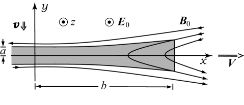
Figure 1: Reconnecting current layer and field lines.

The input parameters are electron number density $n_{0}$ outside the layer, the gradient of the magnetic field $h_{0}$ in the vicinity of separator, the inductive electric field $E_{0}$, and the ratio $\xi=B_{y}/B_{x}$ of the transverse and main components of magnetic field. The mass, momentum, and energy conservation lows give the following analytical expressions for the layer parameters:

for the half-thickness,

$$a=1.7\times 10^{6}\times n_{0}^{-1/2},\,\,\mathrm{cm;}$$

for the half-width,

$$b=0.22\times n_{0}^{1/4}\,h_{0}^{-1}\,E_{0}^{1/2}\,\xi^{\,-1/2},\,\,\mathrm{cm;}$$

for the electron temperature,

$$T_{\rm s}=1.8\times 10^{12}\times n_{0}^{-1/2}\,E_{0}\,\xi^{\,-1},\,\,\mathrm{K;}$$

for the electron density,

$$n_{\rm s}=7.9\times n_{0},\,\,\mathrm{cm}^{-3};$$

for the magnetic field on the inflow sides of the current layer,

$$B_{0}=0.22\times n_{0}^{1/4}\,E_{0}^{1/2}\,\xi^{\,-1/2},\,\,\mathrm{G};$$

for the inflow velocity,

$$v=1.4\times 10^{11}\times n_{0}^{-1/4}\,E_{0}^{1/2}\,\xi^{\,1/2},\,\,\mathrm{cm\,s}^{-1};$$

for the outflow velocity,

$$V=1.7\times 10^{10}\times n_{0}^{-1/4}\,E_{0}^{1/2}\,\xi^{\,-1/2},\,\,\mathrm{cm\,s}^{-1};$$

and for the heating time, which is the time for a given magnetic tube to be connected to the SHTCL,

$$t_{\mathrm{h}}=\frac{2b}{V}=2.6\times 10^{-11}\times n_{0}^{1/2}\,h_{0}^{-1}\,,\,\,s.$$

Table 1 presents two sets of input parameters, which are specific to solar flares, and corresponding output values. We consider two input sets to emphasize the diagnostic capabilities of our models. In the Set 2, only the electric field is decreased when compared with the Set 1. This leads to decreasing the temperature $T_{\mathrm{s}}$, while the heating time $t_{\mathrm{h}}$ is not changed. Both these parameters are important for our further computations of plasma heating by the SHTCL.

The input and output parameters agree with the following observational and theoretical results. The electron number density is consistent with statistical data from the overview of flares by (Caspi 2010): $(0.8-30)\times 10^{10}\leavevmode\nobreak\ \mathrm{cm}^{-3}$. Fig. 5.5 of that work (page 70, right panel) presents densities of super-hot plasma versus maximum RHESSI temperatures that can be as high as 45-50 MK. We note that they are estimated using an isothermal approach. The multitemperature method gives higher temperatures of some portion of plasma.

The electric field agrees with estimations by Somov et al. (2008), Lin (2011): $E_{0}\sim 10-30\leavevmode\nobreak\ \mathrm{V\,cm}^{-1}\approx 0.03-0.1\leavevmode\nobreak\ \mathrm{CGSE}$. The ratio $\xi$ belongs to the range of values where the current layer is stable (Somov & Verneta 1993).

Magnetic fields up to 350 G are expected in coronal sources (Caspi 2010, Fletcher et al. 2011). We assume that these fields are in the magnetic-reconnection region, which is in the vicinity of a separator at heights up to $\sim 4\times 10^{9}$ cm. At present, there are no reliable direct measurements of the coronal magnetic fields. Our theoretical estimations show that magnetic fields can achieve even higher values, up to 900 G, at the separator (Oreshina & Somov, 2009).

We note that the thickness of the layer is very small, and hence, magnetohydrodynamics (MHD) is not a good approximation. We should solve the kinetic equation, but this significantly complicates the model. Instead, we use anomalous transport coefficients, thus considering the deviation from the MHD. Relaxation heat flux (Eq. 4) is also due to the deviation from the Maxwell distribution function.

Table 1: Two sets of parameters for the current layer model

	Set 1	Set 2
Input parameters
$n_{0},\,\,\mathrm{cm}^{-3}$	$10^{10}$	$10^{10}$
$h_{0},\,\,\mathrm{G\,\,cm^{-1}}$	$1.2\times 10^{-6}$	$1.2\times 10^{-6}$
$E_{0},\,\,\mathrm{CGSE}$	$0.1$	$0.0425$
$\xi=B_{y}/B_{x}$	$0.005$	$0.005$
Output parameters
$a,\,\,\mathrm{cm}$	$17$	$17$
$b,\,\,\mathrm{cm}$	$2.6\times 10^{8}$	$1.7\times 10^{8}$
$T_{\mathrm{s}},\,\,\mathrm{K}$	$3.5\times 10^{8}$	$1.5\times 10^{8}$
$n_{\mathrm{s}},\,\,\mathrm{cm}^{-3}$	$7.9\times 10^{10}$	$7.9\times 10^{10}$
$B_{0},\,\,\mathrm{G}$	$312$	$204$
$v,\,\,\mathrm{cm\,s}^{-1}$	$9.6\times 10^{6}$	$6.3\times 10^{6}$
$V,\,\,\mathrm{cm\,s}^{-1}$	$2.4\times 10^{8}$	$1.6\times 10^{8}$
$t_{\mathrm{h}},\,\,\mathrm{s}$	$2$	$2$

2.2 Plasma heating

Let us now consider heating the surrounding plasma by the SHTCL. Due to conversion of magnetic-field energy, the layer temperature is very high, of about $3\times 10^{8}\leavevmode\nobreak\ \mathrm{K}$ (Table 1). When a magnetic tube comes into contact with the layer, plasma inside is heated. While the tube moves from the center to the edge of the layer, a large amplitude heat wave travels along it. After the disconnection from the heating source, the tube continues to move in the corona. Now, only the energy redistribution occurs inside it.

The properties of these thermal waves are complex because of hydrodynamic flows of emitting plasma and kinetic phenomena in it (Somov 1992, Ch. 2). Here, we consider the simplified model to emphasize the main effect, heat conduction. This process can be described by a simple equation (Somov 1992, p. 169):

$$\frac{\partial\,\varepsilon}{\partial\,t}\,=-\,\mathrm{div}\>{\@vec{F}},$$ (2)

where $\@vec{F}$ is the thermal energy flow density, and $\varepsilon$ is the internal energy of unit plasma volume, which is the energy of chaotic motion of particles. We consider only the electron heating because the timescale of the thermal wave propagation is too short to heat ions. Indeed, the time of collisions for electrons is (e.g. Somov 2006a, Sect. 8.31, p. 142)

$$\tau_{\rm ee}=\frac{m_{\rm e}^{2}\,(3\,k_{{}_{\rm B}}T_{\rm e}/m_{\rm e})^{3/2}}{\pi\,e_{\rm e}^{4}\,n_{\rm e}\,(8\,{\rm ln}\Lambda)}\,\frac{1}{0.714}\,,$$

where $m_{\rm e}$, $e_{\rm e}$, $n_{\rm e}$, and $T_{\rm e}$ are the respective electron mass, charge, density, and temperature; $k_{{}_{\rm B}}$ is the Boltzmann constant; and ${\rm ln}\Lambda={\rm ln}\left(9.44\times 10^{\,6}\,T_{\rm e}/n_{\rm e}^{\,\,1/2}\right)$ is the Coulomb logarithm for $T_{\rm e}>5.8\times 10^{5}$ K. The ion collision time is

$$\tau_{\rm ii}=\frac{m_{\rm i}^{2}\,(3\,k_{{}_{\rm B}}T_{\rm i}/m_{\rm i})^{3/2}}{\pi\,e_{\rm i}^{4}\,n_{\rm i}\,(8\,{\rm ln}\Lambda)}\,\frac{1}{0.714}\,,$$

where $m_{\rm i}$, $e_{\rm i}$, $n_{\rm i}$, and $T_{\rm i}$ are the respective ion mass, charge, density, and temperature. The characteristic time of temperature equalizing between the electron and ion components in plasma is

$$\tau_{\rm ei}=\frac{m_{\rm e}\,m_{\rm i}\,(3\,k_{{}_{\rm B}}(T_{\rm e}/m_{\rm e}+T_{\rm i}/m_{\rm i})^{3/2}}{(6\,\pi)^{1/2}\,e_{\rm e}^{2}\,e_{\rm i}^{2}\,n_{\rm i}\,(8\,{\rm ln}\Lambda)}\,.$$

Therefore, we get $\tau_{\rm ee}\sim 1$ s, $\tau_{\rm ii}\sim 50$ s, and $\tau_{\rm ei}\sim 1100$ s for the electron and proton components of plasma with temperature $\sim 10^{8}$ K and density $\sim 10^{10}$ cm^-3. Thus, Coulomb collisions between electrons in the vicinity of the SHTCL are much more frequent than between protons; energy exchange between electrons and protons is very slow. The thermodynamic equilibrium is achieved first for electrons, then for protons, and finally for the whole plasma.

Thus, the internal energy in Eq. (2) is

$$\varepsilon=\frac{3}{2}\,n_{\mathrm{e}}k_{{}_{\mathrm{B}}}T\,,$$ (3)

where $T$ is the electron temperature. This state may not be reached in the conditions under consideration. We use Eq. 3 to define the effective temperature. In the frame of kinetic theory, it is a measure of the width of the electron distribution function in velocity space (Somov 2006a, p. 171).

Various types of heat flux in the SHTCL vicinity have been considered in detail by Oreshina & Somov (2011). The classical Fourier expression ${\@vec{F}}=-\kappa\nabla T$ is not valid here, because it is derived for plasma in a state close to local thermodynamic equilibrium. The latter suggests that the characteristic timescale of the process is much longer than the electron collision time $\tau_{\rm ee}$ and the characteristic length scale exceeds greatly the electron mean free path $\lambda_{\rm ee}$. These conditions are violated at the temperature of about $10^{8}$ K. The thermal wave is too fast and has too steep front, so that the characteristic time of the wave propagation $t_{T}=\frac{T}{\partial T/\partial t}$ is less than $\tau_{\rm ee}$, and the characteristic length scale $l_{T}=\frac{T}{\partial T/\partial l}$ is less than $\lambda_{\rm ee}$ by $1-3$ orders of magnitude. The corresponding plots are presented in the paper by Oreshina & Somov (2011).

We also have showed that there is a generalization of the classical Fourier law, which is better suited to solar flares. It is described by Moses & Duderstadt (1977), who applied it to a laser heated plasma. A general consideration of the problem can be found in (Shkarovskii et al. 1969; Golant et al. 1977). The method is developed in a fundamental framework and is physically substantiated. It is not restricted to slow time variations in the distribution function and thus better suited to the treatment of rapidly varying thermal processes. The technique is based on the Grad 13 moment equations. The electron distribution function is expanded in terms of Hermite-Chebyshev polynomials. The thirteen moments of the distribution function have a clear physical meaning – namely, the density, velocity, temperature, pressure tensor, and heat flux. The system of equations for them is derived from the Boltzmann equation and includes the mass, momentum, and energy conservation laws, the equation for the pressure tensor, and, finally, the equation for heat flux:

$$\@vec{F}=-\kappa\,\nabla T\,-\,\tau\,\frac{\partial\@vec{F}}{\partial t}\,.$$ (4)

Here, $\kappa$ is the heat conductivity coefficient, $\tau$ is some characteristic relaxation time.

According to Braginskii (1963, v. 1, p. 183),

$$\kappa\,=\,\kappa_{0}\,T^{5/2}\,,\qquad\tau\,=\,\tau_{0}\,\,T^{3/2}\,,$$ (5)

where $\kappa_{0}=1.84\times 10^{\,-5}/\,{\mbox{ln}\,\Lambda}\,.$

The technique for calculating the constant $\tau_{0}$ is described by Oreshina & Somov (2011).

$$\tau_{0}=\frac{2}{3}\frac{k_{{}_{\rm B}}\,\kappa_{0}}{n_{\rm e}\,C_{F}^{\,2}}\,,$$

where $C_{F}$ is determined by equality (1). For the solar flare conditions, we estimate

$$\tau_{0}\approx(0.11-1.3)\times 10^{-11}\,\,\mathrm{s\,K}^{-3/2}.$$

The corresponding relaxation time at the temperature of about $10^{8}$ K is

$$\tau=\tau_{0}\,T^{3/2}\big{|}_{T\sim 10^{8}}\sim 1-10\,\,\mathrm{s}\,.$$

These values are comparable to the time of tube contact with the SHTCL, $t_{\mathrm{h}}\approx 2$ s (Table 1). Therefore, the collisional relaxation of heat flux must be considered in models of plasma heating in solar flares. In the following computations, we use $\tau_{0}=1.3\times 10^{-11}\leavevmode\nobreak\ \mathrm{s\,K^{-3/2}}$.

Thus, we solve both the heat conduction equation (2) and the equation for heat flux (4), which determine the temperature $T(\@vec{r},t)$ and the heat flux $\@vec{F}(\@vec{r},t)$. For simplicity, we take $n_{\mathrm{e}}=\mathrm{const}=10^{10}\leavevmode\nobreak\ \mathrm{cm}^{-3}$. We also assume that magnetic tubes are straight and have a constant cross-sectional area. Equations (2) and (4) are rewritten in one-dimensional form:

$$\frac{3}{2}\,n_{\rm e}k_{{}_{\rm B}}\frac{\partial\,T}{\partial\,t}\,=-\,\frac{\partial\,F}{\partial\,l}\,,$$ (6)

$$F=-\,\kappa_{0}\,T^{5/2}\,\frac{\partial T}{\partial l}\,-\,\tau_{0}\,T^{3/2}\,\frac{\partial F}{\partial t}\,,$$ (7)

where $l$ is a coordinate measured from the layer along the tube. We note that the SHTCL is very thin: the ratio of its thickness to the width is less $3\times 10^{-8}$ (Table 1). Thus, we can neglect its thickness and solve Eqs. (6) and (7) for the following boundary conditions.

1) For the time interval $0\lid t\lid t_{\mathrm{h}}$, one end of the tube is connected to the SHTCL with a temperature $T_{\mathrm{s}}$, and the other end is far away and is maintained at a coronal temperature $T_{0}=10^{6}$ K:

$$T(l,t)\,\big{|}_{\,l=0}=T_{\rm s}\,,\quad T(l,t)\,\big{|}_{\,l\rightarrow\infty}=T_{0}\,.$$ (8)

2) For $t>t_{\mathrm{h}}$, the tube is disconnected from the layer and does not receive any heat from it:

$${F(l,t)\,\big{|}}_{\,l=0}=0\,,\quad T(l,\,t)\,\big{|}_{\,l\rightarrow\infty}=T_{0}\,,$$ (9)

$$Q=\int\limits_{0}^{\infty}T(l,\,t)\,{\rm d}l={\rm const}\,.$$ (10)

Equation (10) is the law of thermal-energy conservation in the tube after the separation from the layer.

The problem was solved numerically. The obtained temperature distributions at consequent moments of time are shown in Fig. 2 by the black curves. The grey curves indicate the corresponding distributions obtained for the classical Fourier law, without the relaxation, $\tau_{0}=0$. The top panel presents the thermal wave for the first SHTCL model (see Table 1) and the bottom panel for the second one. They differ in the temperature of the current layer: $T_{\mathrm{s}}=3.5\times 10^{8}$ K in the first case and $T_{\mathrm{s}}=1.5\times 10^{8}$ K in the second one. We stop computations when the heat wave passes from the layer toward the chromosphere at the distance about $1.9\times 10^{10}$ cm. Thus, the computations were interrupted at $t=9$ s for the first model and at $t=20$ s for the second one. For more details, see Appendix.

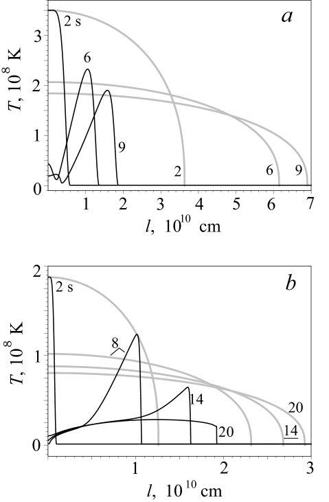
Figure 2: Temperature distributions along a magnetic tube at consequent moments of time, which are obtained with (black curves) and without (grey curves) heat-flux relaxation. (a) $T_{\mathrm{s}}=3.5\times 10^{8}$ K, (b) $T_{\mathrm{s}}=1.5\times 10^{8}$ K. The numbers near the curves denote the time (seconds) passed after the beginning of the tube contact with the SHTCL.

Comparison between the relaxation and classical heat conduction allows us to conclude the following. The relaxation limits the heat flux, making it more realistic. The amount of thermal energy $Q$, supplied to the tube during its contact with the SHTCL, decreases by a factor of 10. The thermal wave slows down as compared to the classical heat conduction. For example, Fig. 2(a) shows that the front velocity is about $3\times 10^{9}\leavevmode\nobreak\ \mathrm{cm\,s}^{-1}$, whereas it is more than the speed of light in the first second of tube contact with the SHTCL in the classical case. The wave shape is also changed after the tube disconnection from the SHTCL. In the relaxation case, the temperature maximum is at the wave front and moves along the tube; a steep front is followed by a smooth decrease. In the classical case, the temperature is at a maximum at the point $l=0$. The relaxation effect decreases in time and the wave shape becomes almost classical (Fig. 2(b)).

Comparison between the cases with different temperature of the layer shows that the amount of heat $Q$ in the tube is less by a factor of 2 in the second model. This result is expected because the temperature of the layer in the second model is $1.5\times 10^{8}$ K instead of $3.5\times 10^{8}$ K in the first model. We note that the temperature behind the wave in the first seconds is close to the background, and we have a solitary wave. In course of time, the temperature behind the wave is increased, and the wave becomes similar to the classic wave about 20 seconds after the disconnection from the layer (Fig. 2(b)). The role of the relaxation is decreased in time.

3 Observational manifestations of the current layer

3.1 Emission measure of the heated plasma

The set of all the magnetic tubes, heated by the SHTCL, is a source of radiation. To compute the emission measure of this heated plasma, we consider a quarter of the tubes, shown by bold lines in Fig. 3. The result is also applicable to the other three quarters if we assume the process to be symmetrical. Let all the tubes be in the $(x,\,y)$-plane and parallel planes within the layer length $L_{z}$. For simplicity, only the tubes in the $(x,\,y)$-plane are shown in Fig. 3. In the layer vicinity, all the tubes are modeled by straight lines, which are inclined at the same angle $\alpha$ to the $(x,\,z)$-plane. In the frames of this model, the magnetic tubes differ from each other only by the time ($t_{1}$, $t_{2}$ … $t_{n}$) passed from their penetrating into the layer.

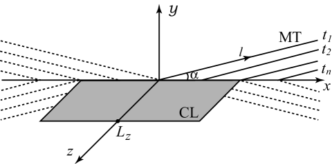
Figure 3: Schematic representation of the radiative source. CL – current layer, MT – magnetic tubes, $t_{1}$, $t_{2}$ … $t_{n}$ – time passed from the tube penetration into the CL, $l$ - coordinate along a tube, $\alpha$ – tube inclination to the CL plane.

By definition, the emission measure of the radiative source is

$$EM=\int\limits_{\mathcal{V}}n_{\mathrm{e}}^{2}\,\mathrm{d}\mathcal{V}\,,$$ (11)

where $\mathcal{V}$ is the volume of the heated plasma. Assuming the tubes are distributed homogeneously along the $z$-axis, Eq. (11) can be rewritten for $x$, $y$, and $z$ coordinates:

$$EM=\int\limits_{x}\int\limits_{y}\int\limits_{z}n_{\mathrm{e}}^{2}\,\mathrm{d}x\,\mathrm{d}y\,\mathrm{d}z\,=\,L_{z}\,\int\limits_{x}\int\limits_{y}n_{\mathrm{e}}^{2}\,\mathrm{d}x\,\mathrm{d}y\,.$$ (12)

The length $L_{z}$ of the SHTCL is a new input parameter. In the following computations, we use $L_{z}=10^{9}$ cm. We replace coordinates $x$ and $y$ by $t$ and $l$; $t$ defines a tube and $l$ is the point on it. These are related by the equalities

$$x = V\,t+l\,\mathrm{cos}\,\alpha\,,$$ (13)

$$y = l\,\,\mathrm{sin}\,\alpha\,,$$ (14)

where $V$ is the velocity of tube movement along the $x$-axis. The Jacobian of this transformation is

$$\left|\begin{array}[]{cc}\displaystyle\frac{\partial x}{\partial t}&\displaystyle\frac{\partial x}{\partial l}\\[11.38109pt] \displaystyle\frac{\partial y}{\partial t}&\displaystyle\frac{\partial y}{\partial l}\end{array}\right|=\left|\begin{array}[]{cc}\vphantom{\displaystyle\frac{\partial x}{\partial t}}V&\mathrm{cos}\,\alpha\\[11.38109pt] \vphantom{\displaystyle\frac{\partial x}{\partial t}}0&\mathrm{sin}\,\alpha\end{array}\right|=V\,\mathrm{sin}\,\alpha\,,$$

and the expression (12) for the emission measure takes the form:

$$EM = L_{z}\,\int\limits_{0}^{t}\int\limits_{0}^{l_{\mathrm{f}}}n_{\mathrm{e}}^{2}\,\,(V\,\mathrm{sin}\,\alpha)\,\mathrm{d}l\,\mathrm{d}t\,=$$

$$= L_{z}\,V\,\mathrm{sin}\,\alpha\,\int\limits_{0}^{t}\int\limits_{0}^{l_{\mathrm{f}}}n_{\mathrm{e}}^{2}\,\,\mathrm{d}l\,\mathrm{d}t\,.$$

Here, $l_{\mathrm{f}}$ is a coordinate of the thermal wave front. We note that we have a unique relationship between coordinate $l$ and temperature $T(t,l)$ for every fixed time $t$ (see Sec. 2). Hence,

$$EM = L_{z}V\,\mathrm{sin}\,\alpha\,\int\limits_{0}^{t}\left(\int\limits_{T(t,0)}^{T(t,l_{\mathrm{f}})}n_{\mathrm{e}}^{2}\,\,\frac{1}{\partial T(t,l)/\partial l}\,\mathrm{d}T\right)\mathrm{d}t=$$ (15)

$$= L_{z}V\,\mathrm{sin}\,\alpha\,\int\limits_{0}^{t}\left(\int\limits_{T(t,0)}^{T(t,l_{\mathrm{f}})}\mathrm{dem}(t,T)\,\mathrm{d}T\right)\mathrm{d}t.$$

Function

$$\left.\mathrm{dem}(t,T)\equiv n_{\mathrm{e}}^{2}\,\,\frac{1}{\partial T(t,l)/\partial l}\right|_{l=l(t,T)}$$

is the differential emission measure of a single magnetic tube of unit cross-section. It is determined from the temperature distributions obtained in Sec. 2. The differential emission measure of the heated plasma is

$$DEM(t,T)=\frac{\mathrm{d}\,EM}{\mathrm{d}\,T}=4\,L_{z}V\,\mathrm{sin}\,\alpha\,\int\limits_{0}^{t}\mathrm{dem}(t,T)\,\mathrm{d}t.$$ (16)

Here, the multiplier 4 considers the entire volume of the heated plasma. The differential emission measure for models 1 and 2 (Table 1) are presented in Fig. 4 (a) and (b).

The behavior of the function $DEM(T)$ depends on the parameters of the layer and hence can serve as a diagnostic tool for it. In the first model, we see two local maxima. The narrow maximum at the layer temperature $T\approx 3.5\times 10^{8}$ K is due to the super-hot current layer and exists for every moment. The wide maximum at $T\approx(1-3)\times 10^{7}$ K is gradually formed due to a smooth temperature drop behind the wave front after the tube disconnection from the layer. In the second model, a remarkable maximum is formed at $T\approx(1-3)\times 10^{7}$ K, too. We note that these temperature estimations are usually obtained from observations of super-hot plasma in solar flares (Caspi 2010). The local narrow maximum at the layer temperature $2\times 10^{8}$ K is almost invisible, which makes direct observations of current layers difficult.

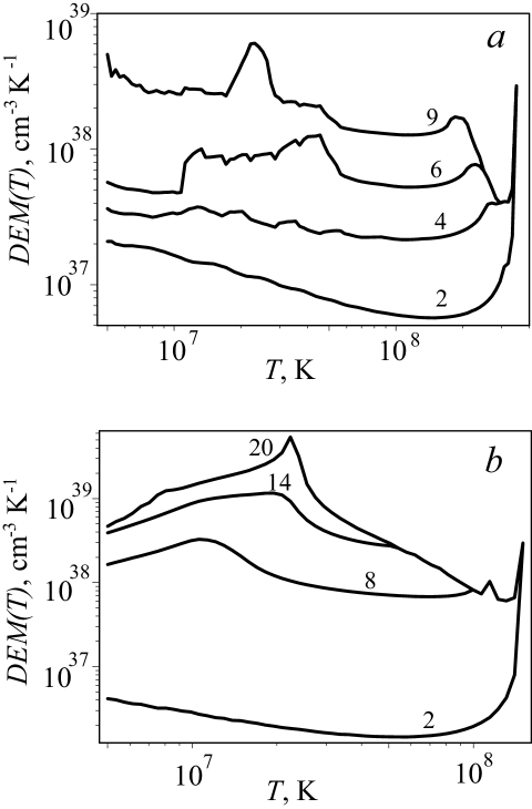
Figure 4: Differential emission measure of the plasma heated by the SHTCL (a) for model 1 and (b) for model 2 (see Table 1). The numbers near the curves denote time (seconds) after the flare start.

Differential emission measure of high-temperature plasma in the M3.5 class flare was determined by Battaglia & Kontar (2012). The authors used the observations of the Solar Dynamic Observatory (SDO) in 94, 171, 211, 335, and 193 Å spectral channels. Thus, they cannot see the super-hot plasma with $T\sim 10^{8}$ K. They consider only the plasma along the line of sight: $DEM=n_{\mathrm{e}}^{2}\,\mathrm{d}l/\mathrm{d}T,\quad\mathrm{cm^{-5}\,K^{-1}}$. Nevertheless, the maximum of $DEM(T)$ around $(1-3)\times 10^{7}$ K seems to be common for our both methods.

Fig. 5 presents the integral emission measure as a function of time:

$$EM(t)=\int DEM(t,T)\,{\mathrm{d}}T\,.$$

Our estimations are consistent by an order of magnitude with RHESSI observations at the beginning of a flare (Liu et al. 2008; Caspi & Lin 2010).

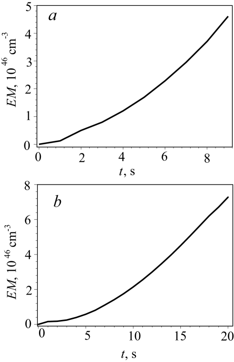
Figure 5: Integral emission measure of the heated plasma (a) for model 1 and (b) for model 2.

3.2 Spectral line intensities

The obtained differential emission measure allows us to compute intensities of spectral lines:

$$I_{\lambda}(t)=\frac{1}{4\,\pi\,R^{2}}\int\frac{P_{\lambda}(T)}{n_{\mathrm{e}}^{2}}\,DEM(t,T)\,\mathrm{d}T,\mathrm{photons\,cm^{-2}\,s^{-1}}.$$ (17)

Here, $R$ (cm) is the distance from the Sun to the Earth, and $P_{\lambda}(T)\leavevmode\nobreak\ (\mathrm{erg\,cm^{-3}\,s^{-1}})$ is the line power, which is the energy radiated by a unit volume of plasma per one second.

The relative power $P_{\lambda}/n_{\mathrm{e}}^{2}$ of 2131 spectral lines in X-rays (1.29–300 Å) are computed over the temperature range $(3\times 10^{4})-10^{9}$ K by Mewe et al. (1985). As we are interested in observing super-hot plasma, we have selected lines with a power maximum at $T\gid 10^{8}$ K. The most powerful lines are Fe xxvi (1.78 Å and 1.51 Å) and Ni xxvii (1.59 Å). They are listed in Table 2 (lines 1–3). The classification of the transitions is given in usual form. ${(P_{\lambda}/n_{\mathrm{e}}^{2})}_{\mathrm{max}}$ is the maximum power value, reached at the temperature $T_{\mathrm{peak}}$. Figure 6 presents the relative power of the lines as a function of temperature. The super-hot lines 1–3 are shown by black curves.

Table 2: Spectral lines for super-hot plasma observations.

No.	Ion	$\lambda$, Å	Transition	${(P_{\lambda}/n_{e}^{2})}_{\mathrm{max}}$,	$T_{\mathrm{peak}}$,
				$\leavevmode\nobreak\ 10^{-25}\mathrm{erg\,cm^{3}\,s^{-1}}$	$10^{8}$ K
1	Fe xxvi	1.780	$1s\,g2S1/2-2p\,\,2P1/2,3/2$	2.9	1.58
2	Fe xxvi	1.510	$1s\,g2S1/2-3p\,\,2P1/2,3/2$	0.42	1.58
3	Ni xxvii	1.590	$1s^{2}\,g1S0-1s2p\,\,1P1$	0.19	1.00
4	Fe xxv	1.851	$1s^{2}\,g1S0-1s2p\,\,1P1$	3.5	0.63
5	Fe xxv	1.858	$1s^{2}\,g1S0-1s2p\,\,3P2,1$	1.23	0.63
6	Fe xxiv	1.864	$1s^{2}2p-1s2p^{2},\,\,1s2s^{2}$	1.10	0.34
7	Fe xxv	1.869	$1s^{2}\,g1S0-1s2s\,\,3S1$	1.00	0.63
8	Fe xxv	1.570	$1s^{2}\,g1S0-1s3p\,\,1P1$	0.52	0.79
9	Fe xxv	1.510	$1s^{2}\,g1S0-1s4p\,\,1P1$	0.20	0.79
10	Fe xxv	1.790	$1s2l-2p2l$ ($l=s,p$)	0.18	0.79

There are many other lines in the spectral vicinity of the super-hot lines 1–3, which are close in power but radiate at the lower temperatures, $T_{\mathrm{peak}}<10^{8}$ K (lines 4–10 in Table 2, grey curves in Fig. 6). For example, the difference between the strongest lines of the two groups is $\lambda_{1}-\lambda_{4}=0.071\leavevmode\nobreak\ \mathrm{\AA}$. Thus, it would be very valuable to have spectral resolution that allows one to separate these lines from each other. For fruitful SHTCL observations, the spectral resolution must be better 0.01 Å. The spacecraft-borne instruments, such as X-ray crystal spectrometers onboard the NASA Solar Maximum Mission and Japanese Hinotori spacecraft, have even better resolution, allowing one to resolve Ly_α lines from hydrogenic iron, $1s^{2}S_{1/2}-2p^{2}P_{3/2}$ and $1s^{2}S_{1/2}-2p^{2}P_{1/2}$ that occur at 1.778 and 1.783 Å.

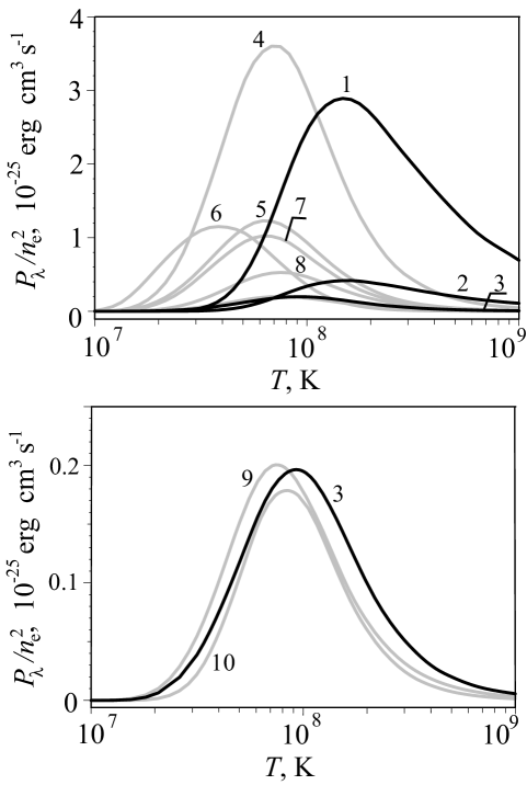
Figure 6: Relative line power as a function of temperature, drawn using the table by Mewe et al. 1985. The numbers near the curves denote the spectral lines according to Table 2. The black curves correspond to the super-hot spectral lines with $T_{\mathrm{peak}}\geq 10^{8}$ K and the grey curves to the lower-temperature ones with $T_{\mathrm{peak}}<10^{8}$ K. The weakest lines 3, 9, and 10 are also shown separately on the bottom panel.

Moreover, the sensitivity of the detectors should be sufficient to record weak photon fluxes. Figure 7 shows the intensities of the super-hot lines $1-3$ (black curves) computed using Eq. (17). They are faint. Only the resonance line 1 has intensity $I_{\lambda}\sim 0.1-2\leavevmode\nobreak\ \mathrm{photons}\,\mathrm{cm}^{-2}\,\mathrm{s}^{-1}$ whereas line 3, for example, is characterized by $I_{\lambda}\sim 0.01-0.1\leavevmode\nobreak\ \mathrm{photons}\,\,\mathrm{cm}^{-2}\,\mathrm{s}^{-1}$.

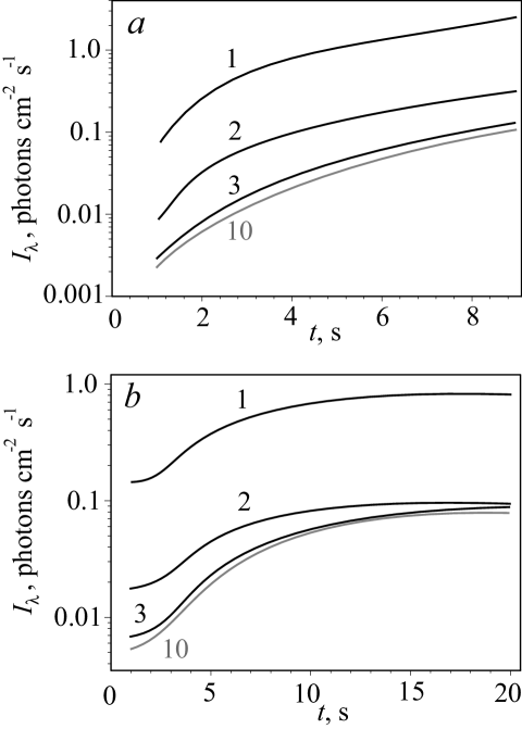
Figure 7: Dependence of intensities of the super-hot spectral lines on time (a) for set 1 of SHTCL parameters and (b) for set 2. The numbers near the curves denote the spectral lines, according to Table 2.

We note that the line power $P_{\lambda}$ was calculated by Mewe et al. (1985) under the assumption of ionization equilibrium; that is the ionization rate from the stage $j$ to $j+1$ is equal to the recombination rate from $j+1$ to $j$:

$$n_{\rm e}\,N_{j}\,Q_{j}=n_{\rm e}\,N_{j+1}\alpha_{j+1}\,,$$

where $Q_{j}$ and $\alpha_{j}$ are the rate coefficients of ionization and recombination from the ionization stage $j$. The ionization state $N_{j}$ of an ion does not depend on the ion temperature $T_{\rm i}$, but it is a function of the electron temperature $T_{\rm e}$. We can estimate the characteristic times of ionization and recombination using the formulas by Phillips (2004):

$$\tau_{\rm ion}=\frac{1}{Q_{j}\,n_{\rm e}}\,,\qquad\tau_{\rm rec}=\frac{1}{\alpha_{j}\,n_{\rm e}}\,.$$

$Q_{j}$ and $\alpha_{j}$ were computed using the method by Arnaud & Raymond (1992). We do not present here the formulas, because they are very cumbersome. For ions Fe xxv and Fe xxvi at the temperature $T_{\rm e}\sim 10^{8}$ K and density $n_{\rm e}\sim 10^{10}$ cm^-3, we obtain $\tau_{\rm ion}\sim\tau_{\rm rec}\sim 100$ s. Thus, the ionization equilibrium is not achieved during rapid plasma heating in the vicinity of SHTCL. That is why the intensities in Fig. 7 can be considered only as a zero-order approximation, an upper limit.

Meanwhile, Dubau et al. (1981) and Pike et al. (1996) show that the Fe xxv satellites can be very useful despite they are faint. They are formed at 1.79 Å   due to transitions $1s2l-2p2l$ ($l=s,p$). The ratio of Fe xxv satellites to Fe xxvi Ly_α lines (1.780 Å) is independent of ionization balance but is a function of temperature (Fig. 8). The role of the low-temperature satellite line Fe xxv relative to the the super-hot resonance line Fe xxvi decreases significantly in increasing $T$.

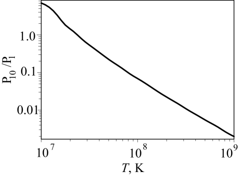
Figure 8: Ratio of powers of the satellite line Fe xxv, 1.790 Å, (No. 10 in Table 2) to the resonance line Fe xxvi, 1.780 Å, (No. 1 in Table 2) as a function of temperature, computed using data by Mewe et al. (1982).

Observations provide us intensities of spectral lines. Their interpretation is not easy, because it depends on the $DEM(T)$ (Eq. 17). Very often the emission source is assumed to be isothermal. Then the intensity ratio equals the power ratio:

$$\frac{I_{10}}{I_{1}}=\frac{P_{10}}{P_{1}}=f(T)\,.$$

Knowing the intensity ratio from observations, we can determine the plasma temperature using Fig. 8.

Let us consider the results obtained in the frame of this isothermal approach on the basis of our theoretical intensities. Figure 9 demonstrates computed Fe xxv/Fe xxvi intensity ratio for models 1 (a) and 2 (b). The plasma is very hot, which leads to a low intensity ratio $\approx 0.022-0.042$ for the first model. Using Fig. 8, we obtain the temperature $T\approx 1.5\times 10^{8}$. It is a good approximation, but the difficulty consists in the faint intensity $I_{10}$ (fig. 7, grey curves): $I_{10}\la 0.1\leavevmode\nobreak\ \mathrm{photons}\,\mathrm{cm}^{-2}\,\mathrm{s}^{-1}$.

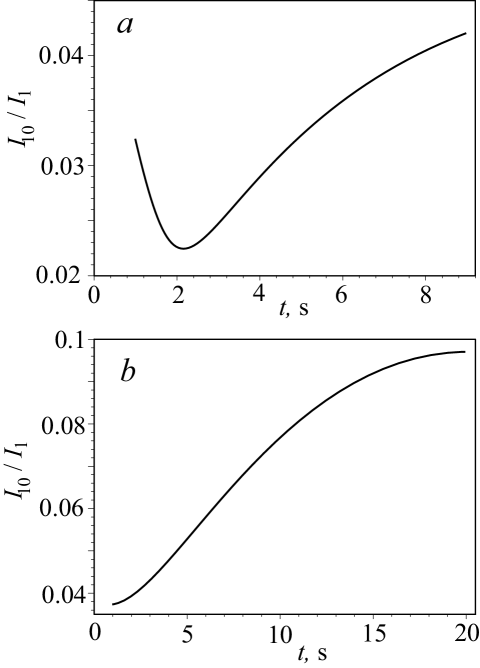
Figure 9: Ratio of intensities of the satellite line Fe xxv, 1.790 Å, (No. 10 in Table 2) to the resonance line Fe xxvi, 1.780 Å, (No. 1 in Table 2) (a) for model 1 and (b) for model 2.

In model 2, the plasma is relatively cooler and the ratio $I_{10}/I_{1}$ is higher: $0.04-0.1$. It corresponds to the temperature change from $1.5\times 10^{8}$ K at the first few seconds to $5\times 10^{7}$ K at $t\approx 20$ s. At the very beginning of a flare, it is very difficult to register $I_{10}$, because its intensity is less than $0.01\leavevmode\nobreak\ \mathrm{photons}\,\mathrm{cm}^{-2}\,\mathrm{s}^{-1}$. For example, Yohkoh observed these lines had integration time periods that were too long, from 24 seconds to 20 minutes (Pike et al. 1996). However, the inferred temperature at 20 s is about $5\times 10^{7}$ K and decreases in time. Thus, we do not obtain temperatures that are more than $10^{8}$ K, even when they are present in the current layer. Theoretically, we can observe these lines, but we need a better telescope. Rough estimations are the following. To detect at least one photon per second from the satellite line with the intensity of about $I_{10}\sim 0.01\leavevmode\nobreak\ \mathrm{photons}\,\mathrm{cm}^{-2}\,\mathrm{s}^{-1}$, we need the effective area of a telescope of about 100 cm². This is problematic. We note, however, that even a comparison between data of Yohkoh and a new instrument having better (not the best) characteristics (effective area, sensitivity of detectors, etc.) can give the right trend for detecting the higher temperatures in flares: the better characteristics, the higher inferred temperatures in large flares.

Thus, observation of multitemperature and nonequilibrium effects in flare plasma are difficult at present, because they are very small. Sometimes, they are not distinguished from instrumental effects (e.g. Holman et al. 2011, Kontar et al. 2011). To eliminate this ambiguity or because of different aims of the work, the majority of observers study mean plasma characteristics, which are much more reliable. For example, Phillips et al. (2006) mostly analyze the flare decay phase, when the temperature is slowly varying “to minimize instrumental problems with high count rates and effects associated with multitemperature and nonthermal spectral components”. The authors, however, note that the isothermal model gives poor spectral fits near the flare maximum. They write that it can be due to deviation of the emitting plasma from the isothermal state. Thus, we can sometimes see evidence of the multitemperature nonequilibrium plasma, which should be studied very carefully.

A more accurate approach than an isothermal one is described by Doschek & Feldman (1987). They determine temperature structure of the radiation source using 16 spectral lines of ions S xv, Ca xix, Ca xix, Fe xx, Fe xxv, Fe xxvi, and Ni xxvii. The analysis demonstrates the possible existence of a super-hot component that extends up to several hundred million degrees. The fraction of the emission measure of the super-hot component to the emission measure of the lower temperature component is low, $\la 0.05-0.1$. This conclusion may be considered as an indirect confirmation for a SHTCL.

4 Conclusions

We describe an analytical model of high-temperature turbulent-current layer. It is shown that the thickness of the layer is very small, of about a few tens of centimeters, whereas the width and the length are about $10^{9}$ cm. Its temperature can be as high as $3\times 10^{8}$ K. This model allows us to compute the temperature distribution in the vicinity of the SHTCL at the beginning of a solar flare. The model considers only heat conduction, the main effect. Its analysis shows that the classical collisional approach is not valid under conditions of solar flare, because we deal with processes that are too fast and wave fronts that are too steep. For a more accurate description, we considered the heat-flux relaxation (Oreshina & Somov 2011). It significantly changes the form of the thermal wave, slows down the front velocity, and decreases the heat input in a magnetic tube during its contact with the SHTCL.

Using the obtained temperature distributions in the vicinity of the layer, we compute the observable characteristics of the plasma in solar flares: differential and integral emission measure and intensity of some spectral lines. These values are computed for two sets of input parameters for the SHTCL models. The difference between the results demonstrates the diagnostic capabilities of our method, which creates a theoretical basis for determining characteristic values of the current layer from future observations.

Particular attention is given to lines of high-charged ions Fe xxvi ($\lambda=1.780$ Å), Fe xxvi ($\lambda=1.510$ Å), and Ni xxvii ($\lambda=1.590$ Å), which are formed at $T\gid 10^{8}$ K. Their observations can be very useful for detecting SHTCLs at the pre-impulsive stage, when the heat conduction is usually a dominant process. The later effects, such as plasma heating by accelerated particles, magnetic traps, chromospheric evaporation, etc., can significantly complicate the data and their interpretation. However, the difficulty consists in the weak intensities of spectral lines at first seconds.

The ratio of the Fe xxv satellite line ($\lambda=1.790$ Å) to the Fe xxvi resonance line ($\lambda=1.780$ Å) is of particular interest, because it does not depend on the ionization balance. This ratio is often used to determine the plasma temperature using an isothermal approach. We show that this technique gives high temperatures ($>10^{8}$ K) only at the very beginning of a flare (about seconds) and then the inferred temperature rapidly decreases. Meanwhile, early observations are difficult because of a very weak Fe xxv satellite line. We expect one photon per cm² during a few tens of seconds. The integration time of actual detectors is about some tens of seconds and more. It can be one of the causes why the inferred temperatures do not exceed $5\times 10^{7}$ K, whereas plasma with $T\ga 10^{8}$ K is present in a flare.

The other reason why these temperatures are not reported is that the isothermal approach for interpreting observations (e.g., Phillips 2004, Phillips et al. 2006, Holman et al. 2011, Kontar et al. 2011) gives volume-averaged temperatures. It is a good method to determine the mean characteristics of flare plasma. Thus, it gives maximum temperatures of about $30-50$ MK. However, Phillips (2004), for example, writes at the end of Sect. 4: “An isothermal plasma is implicit in equations (1), (2), and (4) and in the discussion so far, but more realistically the plasma has a nonthermal temperature structure, describable by a differential emission measure (DEM), $\phi(T_{e})=N_{e}^{2}\,dV/dT_{e}$… .”

We emphasize that the aim of our work is to find the evidence of the SHTCLs. It is an effect of the second order as compared to the mean plasma characteristics, because a percentage of the super-hot ($T\ga 10^{8}$ K) plasma in flares is small. As we can see from Fig. 4 of our paper, the differential emission measure has a main maximum at the temperatures of about 10-30 MK. That is, there is much more plasma in flares at the temperature of 10-30 MK. These values agree well with the isothermal estimations. Only a small peak of $DEM(T)$ at $T\ga 10^{8}$ K is due to the SHTCL. Finding it from observations is not an easy task. The isothermal approach for interpreting observations is very fruitful to determine the general, mean characteristics of the flare plasma, but it is not appropriate for our purposes. We have to consider namely multitemperature and nonequilibrium effects.

Therefore, for the SHTCL diagnostic, the observations in the X-ray range of 1.5–1.8 Å with high spectral resolution (better than 0.01 Å) and high temporal resolution (seconds) are needed. It is also very important to interpret the observations using a multitemperature approach.

Appendix A Length of magnetic-field tubes

The maximal length of magnetic-field tubes ($1.9\times 10^{10}$ cm) is estimated by the following manner. Let us consider a Bastille Day Flare as an example. A magnetic-charges model of this flare was described by Oreshina & Somov (2009).

Fig. 10 presents MDI/SOHO magnetograms for AR NOAA 9077, model magnetograms for the same AR, and a separator. The energy release could be explained by reconnection on two separators: one connects the null points X1 and X2, while the other connects the null points X1 and X3 in the plane of the charges.

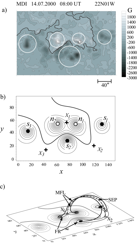
Figure 10: (a) MDI/SOHO magnetograms for AR NOAA 9077; the magnetic field strength on the isolines is shown in gausses. (b) Model magnetograms for the same AR with the same isolines: n1 and n2 are the north-polarity sources; s1, s2, and s3 are the south-polarity sources, and X1, X2, and X3 are the null points. (c) Separator X1X3 (SEP, dashed black line), magnetic field lines in its vicinity (MFL, black lines), and flare ribbons (FR).

Both separators have approximately the same length. As it can be seen from the figure, the distance between the endpoints of each separator is about 56 pixels of MDI, that corresponds to $8.2\times 10^{9}$ cm. In the first approximation, a separator can be considered as a semicircle. Hence, its top is situated at the height $R=4.1\times 10^{9}$ cm. The distance along the separator from the top to the photosphere is $L_{s}=\pi R\,/2=6.4\times 10^{9}$ cm.

The peculiarity of the separator is that it separates different magnetic fluxes. Most of the magnetic-field lines are spread from it and reach the photosphere far from its endpoints. Thus, a heat wave going from the current layer to the photosphere along a field line overcomes the distance much greater than the length of a separator (Fig. 10). It is illustrated also, for example, in the book by Somov (2006b, fig. 3.7, p. 58).

Thus, the path of heat-wave travelling from the current layer to the photosphere can be 2-3 times greater than the half-length of the separator, it can achieve the value $l=L_{s}\times 3=1.9\times 10^{10}$ cm.