Random Matrix Systems with Block-Based Behavior and Operator-Valued Models

Abstract

A model to estimate the asymptotic isotropic mutual information of a multiantenna channel is considered. Using a block-based dynamics and the angle diversity of the system, we derived what may be thought of as the operator-valued version of the Kronecker correlation model. This model turns out to be more flexible than the classical version, as it incorporates both an arbitrary channel correlation and the correlation produced by the asymptotic antenna patterns. A method to calculate the asymptotic isotropic mutual information of the system is established using operator-valued free probability tools. A particular case is considered in which we start with explicit Cauchy transforms and all the computations are done with diagonal matrices, which make the implementation simpler and more efficient.

1 Introduction

Random matrices and free probability are areas of applied probability with increasing importance in the area of multiantenna wireless systems, see for example [5]. One key problem in the stochastic analysis of these systems has been the study of their asymptotic performance with respect to the number of antennas. The first answer to this question is the groundbreaking work by Telatar [14], who, describing the system as a random matrix with statistically independent entries, showed that the capacity of this system is infinite. Since this independence condition might be restrictive, several further proposals have been made over the past decade. As a result, a few models have emerged to take into account some instances of correlation in the system [8], [7], [15].

Operator-valued free probability theory has proved to be a powerful tool to study block random matrices [2, 11]. This has made possible to analyze certain systems exhibiting some block-based dynamics [6, 12]. With recent developments in operator-valued free probability theory [3, 4], simple matricial iterative algorithms now allow us to find the asymptotic spectrum of sums and products of free operator-valued random variables.

The purpose of the present paper is show the significance of these new tools by studying a particular application in wireless communications. In particular, we study an operator-valued Kronecker correlation model based on an arbitrarily correlated finite dimensional multiantenna channel. From a block matrix dynamics and a parameter related to the angle diversity of the system, an operator-valued equivalent is derived and then a method to calculate the asymptotic isotropic mutual information is developed using tools from operator-valued free probability. The model allows using information related to the asymptotic antenna patterns of the system. To our best knowledge, this the first time that a model with these characteristics is analyzed.

More precisely, a multiantenna system is an electronic communication setup in which both the transmitter and the receiver use several antennas. The input and the output of the system can be thought of as complex vectors $u=(u_{1},\cdots,u_{n_{T}})^{\top}$ and $v=(v_{1},\cdots,v_{n_{R}})^{\top}$, where $n_{T}$ is the number of transmitting antennas and $n_{R}$ is the number of receiving antennas. The system response is characterized by the linear model

$$v=Hu+w,$$

where $H$ is an $n_{R}\times n_{T}$ complex random matrix that models the propagation coefficients from the transmitting to the receiving antennas and $w$ is a circularly symmetric Gaussian random vector with independent identically distributed unital power entries.

In a correlated multiantenna system, there is correlation between the propagation coefficients. Namely, the random matrix $H$ is such that the random variables $\{H_{i,j}:i=1,\ldots,n_{R};j=1,\ldots,n_{T}\}$ are not necessarily independent. It is customary to take the random variables composing $H$ with circularly symmetric Gaussian random law [14]. In this context, the joint distribution of the entries of $H$ depends only on the covariance function $\sigma(i,j;i^{\prime},j^{\prime}):=\mathbb{E}\left(H_{i,j}\overline{H}_{i^{\prime},j^{\prime}}\right)$ for $i,i^{\prime}\in\{1,\ldots,n_{R}\}$ and $j,j^{\prime}\in\{1,\ldots,n_{T}\}$.

For a fixed rate $n_{T}/n_{R}$, it is known that the capacity of a multiantenna system grows linearly with the number of antennas of the system as long as the matrix $H$ has independent entries [14]. This shows the well-behaved scalability properties of multiantenna systems. However, correlation may have a negative effect on the performance of the system. Therefore, it is necessary to estimate quantitatively the effect that correlation may have.

Throughout this paper we will assume that the transmitter uses an isotropical scheme, i.e., $\mathbb{E}\left(uu^{\ast}\right)=\dfrac{P}{n_{T}}\mathrm{I}_{n_{T}}$ where $P$ is the transmitter power. In this case, a canonical way to quantify the effect of correlation is by means of the asymptotic isotropic mutual information per antenna [14]. Specifically, suppose that $H_{1}:=H$ and for each $N\geq 2$ the $n_{R}^{(N)}\times n_{T}^{(N)}$ random matrix $H_{N}$ describes the channel behavior when there are $n_{T}^{(N)}$ transmitting antennas and $n_{R}^{(N)}$ receiving antennas. Moreover, suppose that both $(n_{T}^{(N)})_{N\geq 1}$ and $(n_{R}^{(N)})_{N\geq 1}$ are increasing sequences and $n_{T}^{(N)}/n_{R}^{(n)}$ converges to a positive real number. Then, the asymptotic isotropic mutual information per antenna $I_{\infty}$ is

$$I_{\infty}=\lim_{N\rightarrow\infty}\mathbb{E}\left(\frac{1}{n_{R}^{(N)}}\log\det\left(I+\frac{P}{n_{T}^{(N)}}H_{N}H_{N}^{\ast}\right)\right),$$

as long as the limit exists. A common phenomena in random matrix theory is that the sequence of arguments in the expected value above converges almost surely to a constant, and under mild conditions also in mean. Therefore, the asymptotic isotropic mutual information per antenna is given, essentially, by the a.s. limit of the aforementioned sequence.

Therefore, in order to find $I_{\infty}$, it is necessary to derive a model for the sequence of random matrices $(H_{N})_{N\geq 1}$ that approximates the channel behavior in the finite size regime and then compute the asymptotic quantity $I_{\infty}$.

In this paper we use an alternative method described in four steps:

1. Assign an operator-valued matrix $\mathbf{H}$ to the matrix $H$;

2. Compute the operator-valued Cauchy transform of $\mathbf{HH}^{\ast}$;

3. Via the Stieltjes inversion formula, recover the distribution of $\mathbf{HH}^{\ast}$, call it $F$;

4. Compute $I_{\infty}$ as

   $$I_{\infty}=\int\log(1+P\xi)F(\text{d}\xi).$$ (1)

The operator-valued matrix $\mathbf{H}$ can be thought of as the asymptotic operator-valued equivalent of the channel $H$ [12]. In this sense, the common approach consists of giving a model for the finite size regime, computing the mutual information, and taking the limit. On the other hand, the alternative approach takes limits in the model, replacing matrices by operator-valued matrices, and then calculates the mutual information. Of course, these approaches are intimately related. Actually, in the traditional case, they provide the same results, but we prefer the latter approach since it is conceptually easier to understand and carry out, providing a powerful tool for modelling.

We will see that this way of thinking goes well with channels exhibiting a block-based behavior. In particular, the operator-valued matrix assigned in step 1 carries the block structure of the channel and some other features of the system. In the example analyzed here, these features include the effect of the asymptotic antenna patterns and the inclusion of the starting finite dimensional channel correlation. To illustrate the kind of tools that may be useful in the assigning process at step 1, in the next section we retrieve a block-based Kronecker model from an angular-based model and derive the operator-valued equivalent $\mathbf{H}$.

In Section 2 we derive the proposed operator-valued Kronecker correlation model. In Section 3 we discuss the asymptotic isotropic mutual information of our model using tools from operator-valued free probability. In Section 4 we consider a particular example where the implementation is simple but at the same time flexible enough to be applied in several interesting cases, like some symmetric channels. In Section 5 we compare, through the example of a finite dimensional system, the mutual information predicted by the usual Kronecker correlation model against the results from the proposed operator-valued alternative. In Appendix A we summarize the notation, the background, and the prerequisites from operator-valued free probability theory. In Appendix B we prove Theorem 1 on two extreme behaviors of the model regime. In Appendix C we compute some of the operator-valued Cauchy transforms required in this paper.

2 The Angular Based Model and Its Operator-Valued Equivalent

The proposed model to approximate the channel behavior in the finite size regime is derived as follows. Suppose that for a fixed $N\in\mathbb{N}$, each antenna of the original system is replaced by $N$ new antennas located around the position of the original one. Thus, the new system has $n_{T}N$ transmitting and $n_{R}N$ receiving antennas. Figure 1 shows the original system for $n_{T}=1$ and $n_{R}=2$ together with the corresponding virtual one for $N=2$.

Figure 1: On the left the original $1\times 2$ system. On the right the virtual $2\times 4$ system corresponding to $N=2$.

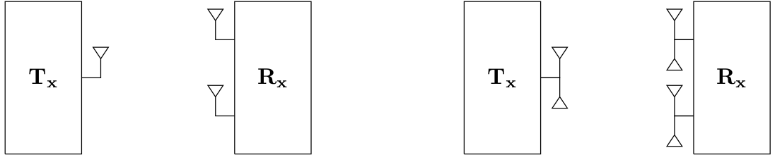
For any given $N\in\mathbb{N}$, the channel matrix $H_{N}$ for this $n_{R}N\times n_{T}N$ system will have the form

$$H_{N}=\left(\begin{matrix}H_{N}^{(1,1)}&\cdots&H_{N}^{(1,n_{T})}\\ \vdots&\ddots&\vdots\\ H_{N}^{(n_{R},1)}&\cdots&H_{N}^{(n_{R},n_{T})}\end{matrix}\right),$$

where $H_{N}^{(i,j)}$ is the $N\times N$ matrix whose entries are the coefficients between the new antennas that come from the original $i$ receiving and $j$ transmitting antennas.

2.1 Statistics of the channel and block matrix structure

We now derive a model for $H_{N}=(H_{N}^{(i,j)})_{i,j}$ that takes into account the statistics of the channel matrix $H$ and the block structure exhibited above. First, fix a block $H_{N}^{(i,j)}$, and for notational simplicity denote it by $A$. This matrix $A$ should reflect the behavior of a scalar channel between two antennas of the original system when these are replaced by $N$ antennas each.

In a regime of a very high density of antennas per unit of space, any two pairs of antennas close enough are likely to experience very similar fading. Since as $N\rightarrow\infty$ the new antennas are closer to each other, then the propagation coefficients between them are prone to be correlated. As an extreme case, we suppose that all the propagation coefficients between the antennas involved in $A$ have the same norm, and without loss of generality we set this to be one. This means that these coefficients produce the same power losses and the differences between them come from the variation that they induce in the signal’s phases. With this in mind, we will suppose that for $1\leq k,l\leq N$,

$$A_{k,l}=\exp(\gamma\mathrm{i}\theta_{k,l})$$

where $\mathrm{i}=\sqrt{-1}$, $\theta_{k,l}$ is a real random variable and $\gamma>0$ is a physical parameter that reflects the statistical variation of the phases of the incoming signals. In some geometrical models, this statistical variation of the phases has been used, along with the angle of arrival and the angle spread, to study the capacity of multiantenna channels [8].

Some of the physical factors that have the most impact on the correlation of an antenna array are related to either the physical parameters of the antennas or to local scatterers. Since these factors are different for each end of the communication link then, borrowing the intuition from the usual Kronecker model, it is natural to take the matrix $\theta=(\theta_{k,l})_{k,l=1}^{N}$ as a separable or Kronecker correlated matrix, that is,

$$\theta=RXT$$

where $R$ and $T$ are the square roots of suitable correlation matrices and $X$ is a random matrix with independent entries having the standard Gaussian distribution. It is important to point out that $A$ is not Kronecker correlated.

2.2 Extreme regimes of the parameter $\gamma$ of the system

From a modelling point of view, the case $\gamma\rightarrow\infty$ represents the situation in which the environment is rich enough to ensure a high diversity in the angles of the propagation coefficients. On the other hand, the case $\gamma\rightarrow 0$ represents a system in which the propagation coefficients in the given block are almost the same. Intuitively, the first case is better in terms of $\gamma$, since we should be able to recover the multiantenna diversity via the angle diversity; while in the second case we almost lose the diversity advantage of a multiantenna system over a single antenna system.

In these limiting cases the following holds. We denote by $\lambda_{1}(\cdot)\geq\cdots\geq\lambda_{N}(\cdot)$ the ordered eigenvalues of an Hermitian matrix.

Theorem 1.

Assume that $R$ and $T$ are full rank. For $N$ fixed, as $\gamma\rightarrow\infty$,

$$(\lambda_{1}(AA^{\ast}),\ldots,\lambda_{N}(AA^{\ast}))\Rightarrow(\lambda_{1}(UU^{\ast}),\ldots,\lambda_{N}(UU^{\ast}))$$

where $U$ is a matrix with i.i.d. entries with uniform distribution on the unit circle.

Suppose that $(\gamma_{N})_{N\geq 1}$ is a sequence of positive real numbers such that $\gamma_{N}\rightarrow 0$ as $N\rightarrow\infty$. Then, almost surely, $F^{\gamma_{N}^{-2}AA^{\ast}}\Rightarrow F$ as $N\rightarrow\infty$ where $F$ is the asymptotic eigenvalue distribution of $\theta\theta^{\ast}$.

Proof.

See Appendix B. ∎

Observe that in the second part of the previous theorem both $A$ and $\theta$ depend on $N$ as they are $N\times N$ matrices.

This means that the entries of the matrix $A$ become uncorrelated as $\gamma\rightarrow\infty$, and, by universality, the spectrum of $A$ must behave similar to the spectrum of a standard Gaussian matrix of the same size. Observe that in this limiting case, we arrive at the well known case of i.i.d. entries, i.e., the canonical model of a multiantenna system [14]. As was mentioned before, in this situation the environment has a high diversity in the angles of the propagation coefficients, and thus it is natural that the system behaves as in the i.i.d. case.

On the other hand, when $\gamma\rightarrow 0$, the bulk of $AA^{\ast}$ is close to that of $\gamma^{2}\theta\theta^{\ast}=\gamma^{2}RXT^{2}XR$. This suggests approximating $A\approx\gamma RXT$. Note that this limiting case leads to the well known Kronecker correlation model [15]. In the spirit of a worst case analysis, we will use $A=\gamma RXT$ in what follows.

Remark 1.

In the proof of Theorem 1 we only used the fact that $\theta\theta^{*}$ has an asymptotic eigenvalue distribution with compact support and $\left|\left|\theta\theta^{*}\right|\right|_{op}$ converges a.s. as $N\to\infty$. Therefore, under these mild conditions, the same analysis yields to the approximation $A=\gamma\theta$ for any model $\theta$.

2.3 Operator-valued free probability modelling

In terms of the asymptotic behavior of the spectrum and invoking ideas from random matrix theory and free probability, let $(\mathcal{C},\varphi)$ be a noncommutative probability space where the algebra $\mathcal{C}$ has unit $\mathbf{1}_{\mathcal{C}}$ (see Appendix A). We can model the matrix $A=\gamma RXT$ by means of a noncommutative random variable $a$ in $\mathcal{C}$ such that $a=rxt$ where $r$ and $t$ are in $\mathcal{C}$ such that $r^{2}$ and $t^{2}$ are the limits in distribution of $R^{2}$ and $T^{2}$ respectively, and $x$ is a circular operator with a given variance. Since the matrices $R^{2}$ and $T^{2}$ depend on separate sides of the communication link, and in some contexts, such as mobile communications, the transmitter and receiver are not in any particular orientation with respect to each other, we can assume that the eigenmodes of this matrices are in standard position. In particular, this means that the distributional properties of $R$ and $T$ are invariant under random rotations, i.e., $(R,T)\overset{\mathrm{d}}{=}(R,UTU^{\ast})$ where $U$ is a Haar distributed random matrix independent from $R$ and $T$. The latter implies that $r$ and $t$ are free [5], and by Voiculescu’s theorem [9] they both are free from $x$.

If we use the noncommutative random variable representation, as we did with $A$, for every block $H_{N}^{(i,j)}$ with $i\in\{1,\ldots,n_{R}\}$ and $j\in\{1,\ldots,n_{T}\}$, then

$$\left(H_{N}^{(i,j)}:i=1,\ldots,n_{R};j=1,\ldots,n_{T}\right)\overset{\textnormal{dist}}{\longrightarrow}\left(r_{i,j}x_{i,j}t_{i,j}:i=1,\ldots,n_{R};j=1,\ldots,n_{T}\right),$$

where $r_{i,j}$, $t_{i,j}$ and $x_{i,j}$ are the corresponding correlation and circular random variables for the block $H_{N}^{(i,j)}$. By the same argument as before, we assume that the families $\{r_{i,j}:i,j\}$ and $\{t_{i,j}:i,j\}$ are free. In this way, for any $m\in\mathbb{N}$

$$\lim_{N\rightarrow\infty}\mathbb{E}\left(\text{tr}_{n_{R}N}\left((H_{N}H_{N}^{\ast})^{m}\right)\right)=(\text{tr}_{n_{R}}\circ E)\left((\mathbf{HH}^{\ast})^{m}\right)$$

where

$$\mathbf{H}=\left(\begin{matrix}r_{1,1}x_{1,1}t_{1,1}&\cdots&r_{1,n_{T}}x_{1,n_{T}}t_{1,n_{T}}\\ \vdots&\ddots&\vdots\\ r_{n_{R},1}x_{n_{R},1}t_{n_{R},1}&\cdots&r_{n_{R},n_{T}}x_{n_{R},n_{T}}t_{n_{R},n_{T}}\end{matrix}\right).$$

Let $\mathrm{I}_{n_{R}}\otimes\text{tr}_{N}:\textnormal{M}_{n_{R}N}\left(\mathbb{C}\right)\rightarrow\textnormal{M}_{n_{R}}\left(\mathbb{C}\right)$ be the linear map determined by

$$(\mathrm{I}_{n_{R}}\otimes\text{tr}_{N})(E_{i,j}\otimes A)=\text{tr}_{N}\left(A\right)E_{i,j}$$

where $E_{i,j}$ is the $i,j$-unit matrix in $\textnormal{M}_{n_{R}}\left(\mathbb{C}\right)$ and $A$ is any $N\times N$ matrix. It is clear that $\text{tr}_{n_{R}N}=\text{tr}_{n_{R}}\circ(\mathrm{I}_{n_{R}}\otimes\text{tr}_{N})$. For every $N\in\mathbb{N}$, $H_{N}H_{N}^{*}$ belongs to the $\textnormal{M}_{n_{R}}\left(\mathbb{C}\right)$-valued probability space $(\textnormal{M}_{n_{R}N}\left(\mathbb{C}\right),\mathbb{E}\circ(\mathrm{I}_{n_{R}}\otimes\text{tr}_{N}))$ and $\mathbf{HH}^{*}$ to the $\textnormal{M}_{n_{R}}\left(\mathbb{C}\right)$-valued probability space $(\textnormal{M}_{n_{R}}\left(\mathcal{C}\right),E)$ where $E:=\mathrm{I}_{n_{R}}\otimes\varphi$.

Moreover, we will restrict ourselves to working with asymptotic eigenvalue distributions with compact support, which allows us to work within the framework of a $C^{\ast}$-probability space. In this context, convergence in distribution implies weak convergence of the corresponding analytic distributions [10], see also Appendix A.

In the derivation of this model, we can observe that all the $r_{k,1},\ldots,r_{k,n_{T}}$ depend on the new antennas around the original $k$th receiving antenna, and thus it is reasonable to take all them equal to some random variable $r_{k}$. Proceeding with this reasoning at the transmitter side, we conclude that

$$\mathbf{H}=\mathbf{RXT}$$ (2)

where $\mathbf{R}=\textnormal{diag}\left(r_{1},\ldots,r_{n_{R}}\right)$ and $\mathbf{T}=\textnormal{diag}\left(t_{1},\ldots,t_{n_{T}}\right)$ are the operators associated to the correlation structure of the antennas at each side, and $\mathbf{X}=(x_{i,j})_{i,j}$. Thus, we can think of this model as the operator-valued version of the Kronecker correlation model for multiantenna systems.

Moreover, let $\Sigma^{2}$ be the correlation matrix of $\textrm{Vec}\left(\mathbf{X}\right)$, i.e., $E\left(\textrm{Vec}\left(\mathbf{X}\right)\textrm{Vec}\left(\mathbf{X}\right)^{\ast}\right)=\Sigma^{2}$. In terms of the model, $\Sigma^{2}$ must reflect the correlation structure of the channel matrix $H$ and the parameter $\gamma$ of the system. A reasonable way to do this is by setting $\Sigma^{2}=\gamma^{2}\mathbb{E}\left(\textrm{Vec}\left(H\right)\textrm{Vec}\left(H\right)^{\ast}\right)$. In the regime $\gamma\rightarrow 0$, the latter implies that the mutual information decreases proportionally to $\gamma^{2}$. Since we can incorporate the constant $\gamma$ into the correlation operator-valued matrices $\mathbf{R}$ and $\mathbf{T}$, for notational simplicity we will set $\gamma=1$ in our discussion, thus we will take $\Sigma^{2}=\mathbb{E}\left(\textrm{Vec}\left(H\right)\textrm{Vec}\left(H\right)^{\ast}\right)$. Nonetheless, remember that the model derivation was made in the regime $\gamma\rightarrow 0$.

Observe that each $r_{k}$ depends on the new antennas around the original $k$th receiving antenna. Thus the distribution of $r_{k}$ will depend strongly on the specific geometric distribution of the new antennas. For example, if all the new antennas are located in exactly the same place as the original antenna, we would obtain that the distribution of $r_{k}$ must be zero. In the case where the antennas are collinear and equally spaced, we can use some class of Toeplitz operators as shown in [7]. A similar argument can be used for the transmission operators.

Remark 2.

Observe that in this way we have incorporated the finite dimensional statistics in our operator-valued equivalent. Moreover, the correlation matrix $\Sigma^{2}$ does not need to be separable, i.e., with a Kronecker structure. This shows that the operator-valued Kronecker model is slightly more flexible than the classical version: it allows an arbitrary correlation resulting from the channel, and it also allows different correlations for different regions of the transmitter and receiver antenna arrays, which in our notation is encoded in the matrices $\mathbf{T}$ and $\mathbf{R}$.

3 Asymptotic Isotropic Mutual Information Analysis

In this section we derive a method to calculate the asymptotic isotropic mutual information (1) of our model using the tools of operator-valued free probability. For simplicity of exposition, in what follows we will take $n_{R}=n_{T}=n$. Note that if, for example, $n_{R}<n_{T}$, then we can proceed by just taking $n=n_{T}$ and by taking $r_{k}$ equal to $0$ for $k>n_{R}$. Let $\mathbf{R}$, $\mathbf{X}$ and $\mathbf{T}$ as in (2). The goal is to find the distribution $F$ of $\mathbf{HH}^{\ast}$ in (1) by means of the $\textnormal{M}_{n}\left(\mathbb{C}\right)$-valued Cauchy transform of $\mathbf{HH}^{\ast}$ (see Appendix A).

Using the symmetrization technique [12], we define $\widehat{\mathbf{H}}$ as

$$\widehat{\mathbf{H}}=\left(\begin{matrix}0&\mathbf{H}\\ \mathbf{H}^{\ast}&0\end{matrix}\right).$$

Notice that the distribution of $\widehat{\mathbf{H}}^{2}$ is the same as the distribution of $\mathbf{HH}^{\ast}$, and that $\widehat{\mathbf{H}}$ is selfadjoint. Since all the odd moments of $\widehat{\mathbf{H}}$ are 0, the distribution of $\widehat{\mathbf{H}}$ is symmetric.

We can then obtain the $\textnormal{M}_{2n}\left(\mathbb{C}\right)$-valued Cauchy transform (9) of $\widehat{\mathbf{H}}^{2}$ from the corresponding transform of $\widehat{\mathbf{H}}$ using the formula [10]

$$G_{\widehat{\mathbf{H}}}(\zeta\mathrm{I}_{2n})=\zeta G_{\widehat{\mathbf{H}}^{2}}(\zeta^{2}\mathrm{I}_{2n}),$$

where $\zeta\in\mathbb{C}$ and $\mathrm{I}_{2n}$ is the identity matrix in $\textnormal{M}_{2n}\left(\mathbb{C}\right)$. Since

$$\widehat{\mathbf{H}}=\left(\begin{matrix}\mathbf{R}&0\\ 0&\mathbf{T}\end{matrix}\right)\left(\begin{matrix}0&\mathbf{X}\\ \mathbf{X}^{\ast}&0\end{matrix}\right)\left(\begin{matrix}\mathbf{R}&0\\ 0&\mathbf{T}\end{matrix}\right),$$

the spectrum of $\widehat{\mathbf{H}}$ is the same as the spectrum of

$$\left(\begin{matrix}\mathbf{R}^{2}&0\\ 0&\mathbf{T}^{2}\end{matrix}\right)\left(\begin{matrix}0&\mathbf{X}\\ \mathbf{X}^{\ast}&0\end{matrix}\right)=\mathbf{Q}\widehat{\mathbf{X}}\text{, say}.$$ (3)

The $\textnormal{M}_{2n}\left(\mathbb{C}\right)$-valued Cauchy transform of $\widehat{\mathbf{X}}$ is well known (see [6]). Thus, we just need to find the $\textnormal{M}_{2n}\left(\mathbb{C}\right)$-valued Cauchy transform of $\mathbf{Q}$ in order to be able to apply the operator-valued subordination theory [3, 4]; see (12) in Theorem 5 of the Appendix A.

Remark 3.

a) The above mentioned operator valued subordination theory allows us to compute, via iterative algorithms over matrices, the distribution of sums and products of operator valued random variables free over some algebra (Theorem 5 in Appendix A). For a rigorous exposition of the concept of freeness over an algebra, we refer the reader to [6, 12] and the references therein. Observe that this relation is similar to the usual freeness in free probability.

b) The Cauchy transform of $\widehat{\mathbf{X}}$ is not given explicitly, instead, it is given as a solution of a fixed point equation [6]. In general, the $\textnormal{M}_{2n}\left(\mathbb{C}\right)$-valued Cauchy transform $G_{\widehat{\mathbf{X}}}:\textnormal{M}_{2n}\left(\mathbb{C}\right)\rightarrow\textnormal{M}_{2n}\left(\mathbb{C}\right)$ has to be computed for any matrix $B\in\textnormal{M}_{2n}\left(\mathbb{C}\right)$. However, in some cases it is enough to compute it for diagonal matrices, which simplifies the practical implementation (see Section 4).

If the correlation matrices associated to the correlation operators $\{r_{k}\}$ are either constant or exhibit a distribution invariant under random rotations, as we supposed for $r$ and $t$ in the previous section, then these correlation operators will be free among themselves. In some applications, these correlation operators come from constant matrices since they model the antenna array architecture which in principle is fixed. Suppose that this is the case, and that also the $\{t_{k}\}$ are free among themselves. In some cases this hypothesis will be unnecessary (see Section 4). Observe that

$$\mathbf{Q}=\sum_{k=1}^{n}r_{k}^{2}E_{k,k}+\sum_{k=1}^{n}t_{k}^{2}E_{n+k,n+k}.$$

By the assumed freeness relations between the random variables $\{r_{k},t_{k}\}_{k}$, we have that the coefficients of the operator-valued matrices in the previous sums are free, and thus the operator-valued matrices $\{r_{k}^{2}E_{k,k}:1\leq k\leq n\}\cup\{t_{k}^{2}E_{n+k,n+k}:1\leq k\leq n\}$ are free over $\textnormal{M}_{2n}\left(\mathbb{C}\right)$. So we just have to compute the $\textnormal{M}_{2n}\left(\mathbb{C}\right)$-valued Cauchy transform of each operator-valued matrix in the above sum, and then apply the results from the free additive subordination theory ((11) of Theorem 5 in Appendix A).

Theorem 2.

Let $r$ be a noncommutative random variable, $n\geq 1$ a fixed integer and $k\in\{1,\ldots,n\}$. For $B\in\textnormal{M}_{2n}\left(\mathbb{C}\right)$,

$$G_{rE_{k,k}}(B)=B^{-1}+[B^{-1}]_{k,k}^{-2}\left(G_{r}([B^{-1}]_{k,k}^{-1})-[B^{-1}]_{k,k}\right)B^{-1}E_{k,k}B^{-1}.$$

Proof.

See Appendix C. ∎

With the previous theorem, we can compute the $\textnormal{M}_{2n}\left(\mathbb{C}\right)$-valued Cauchy transforms of $\{r_{k}^{2}E_{k,k},$ $t_{k}^{2}E_{n+k,n+k}\}$. With these transforms, we have all the elements to compute the $\textnormal{M}_{2n}\left(\mathbb{C}\right)$-valued Cauchy transform of $\ \widehat{\mathbf{H}}$, and in consequence the scalar Cauchy transform of the spectrum $F$ of $\mathbf{HH}^{\ast}$ is obtained from (10):

$$G_{F}(\zeta)=\text{tr}_{n_{R}}(G_{\mathbf{HH}^{\ast}}(\zeta\mathrm{I}_{2n}))\mathbf{,\quad}\zeta\in\mathbb{C}\mathbf{.}$$

Using the Stieltjes inversion formula, one then obtains $F$ and this gives the asymptotic isotropic mutual information (1).

4 Channels with Symmetric-Like Behavior

From Section 2, we have that

$$\mathbf{X}=\left(\begin{matrix}x_{1,1}&\cdots&x_{1,n}\\ \vdots&\ddots&\vdots\\ x_{n,1}&\cdots&x_{n,n}\end{matrix}\right)$$

is an operator-valued matrix composed of circular random variables with correlation

$$\Sigma^{2}=\mathbb{E}\left(\textrm{Vec}\left(H\right)\textrm{Vec}\left(H\right)^{\ast}\right).$$

Observe that in this case,

$$\textrm{Vec}\left(\mathbf{X}\right)=\Sigma\left(\begin{matrix}c_{1,1}\\ c_{2,1}\\ \vdots\\ c_{n,n}\end{matrix}\right)$$

where the $c_{k,l}$ ($1\leq k,l\leq n$) are free circular random variables. Thus there exist complex matrices $M_{k,l}$ for $1\leq k,l\leq n$ such that

$$\mathbf{X}=\sum_{k,l=1}^{n}c_{k,l}M_{k,l},$$ (4)

i.e., $\mathbf{X}$ can be written as the sum of free circular random variables multiplied by some complex matrices. In this way, the summands in (4) are free over $\textnormal{M}_{n}\left(\mathbb{C}\right)$. Observe that the previous procedure is exactly the same as writing a matrix of complex Gaussian random variables as a sum of independent complex Gaussian random variables multiplied by some complex matrices.

For $1\leq k,l\leq n$, define

$$\widehat{\mathbf{X}}_{k,l}=\left(\begin{matrix}\mathbf{0}&c_{k,l}M_{k.l}\\ c_{k,l}^{*}M_{k,l}^{*}&\mathbf{0}\end{matrix}\right),$$

so $\widehat{\mathbf{X}}=\sum_{k,l=1}^{n}\widehat{\mathbf{X}}_{k,l}$. Recall that the operator-valued matrices $\{\widehat{\mathbf{X}}_{k,l}\}$ are free over $\textnormal{M}_{2n}\left(\mathbb{C}\right)$. As an alternative to the technique given in [6] to compute the operator-valued Cauchy transform of $\widehat{\mathbf{X}}$, we can use the subordination theory by computing the individual operator-valued Cauchy transforms $G_{\widehat{\mathbf{X}}_{k,l}}$ for all $1\leq k,l\leq n$ and then using equation (11). This technique is particularly neat in the following setup.

Suppose that for all $1\leq k,l\leq n$ the operator-valued Cauchy transforms $G_{\widehat{\mathbf{X}}_{k,l}}$ send diagonal matrices to diagonal matrices. From this assumption and Equations (11) and (12), it follows that this property is also shared by $G_{\widehat{\mathbf{X}}}$. Moreover, the following theorem shows that this is also true for the operator-valued Cauchy transform of $\mathbf{Q}$.

Theorem 3.

Let $D=\textnormal{diag}\left(d_{1},\ldots,d_{2n}\right)$ be a diagonal matrix in $\textnormal{M}_{2n}\left(\mathbb{C}\right)$. Then

$$G_{\mathbf{Q}}(D)=\textnormal{diag}\left(G_{r_{1}}(d_{1}),\ldots,G_{t_{n}}(d_{2n})\right).$$ (5)

Proof.

See Appendix C. ∎

Since this diagonal invariance property is also satisfied by $\mathbf{Q}$, again from Equations (11) and (12), we conclude that $\widehat{\mathbf{H}}$ satisfies this property. Therefore, all the computations involved in this case are within the framework of diagonal matrices.

Also, in this diagonal case, any assumption of freeness between the noncommutative random variables in $\mathbf{R}$ and $\mathbf{T}$ is unnecessary since they do not interact when evaluating the Cauchy transform of $\mathbf{Q}$ in diagonal matrices. Intuitively, the structure of $\mathbf{X}$ behaves well enough to destroy the effect that any possible dependency between the correlation operators may have in the spectrum of $\mathbf{H}$.

It is easy to prove that the condition that $G_{\widehat{\mathbf{X}}_{k,l}}$ sends diagonal matrices to diagonal matrices is equivalent to requiring that

$$\left(\begin{matrix}0&M_{k,l}\\ M_{k,l}^{\ast}&0\end{matrix}\right)J\left(\begin{matrix}0&M_{k,l}\\ M_{k,l}^{\ast}&0\end{matrix}\right)$$

is diagonal for any diagonal matrix $J\in\textnormal{M}_{2n}\left(\mathbb{C}\right)$. This last condition can be shown to be equivalent to requiring that for all $1\leq k,l\leq n$, we have that $M_{k,l}=D_{k,l}P_{k,l}$ where $D_{,lk}$ is a diagonal matrix in $\textnormal{M}_{n}\left(\mathbb{C}\right)$ and $P_{k,l}$ is a permutation matrix.

Remark 4.

If in a concrete application the correlation matrix $\mathbb{E}\left(\textrm{Vec}\left(H\right)\textrm{Vec}\left(H\right)^{\ast}\right)$ can be suitably decomposed, or approximated, in such a way that this latter condition holds, then the method of this example can be applied.

Theorem 4.

Let $n\geq 1$. Suppose that $x$ is a circular random variable, $D$ a diagonal matrix in $\textnormal{M}_{n}\left(\mathbb{C}\right)$, and $P$ a permutation matrix of the same size. Let $M:=DP$ and $\widehat{Mx}:=\left(\begin{smallmatrix}0&Mx\\ M^{\ast}x^{\ast}&0\end{smallmatrix}\right)$. Then, for $J=\left(\begin{smallmatrix}J_{1}&0\\ 0&J_{2}\end{smallmatrix}\right)$ with $J_{1}$ and $J_{2}$ diagonal matrices in $\textnormal{M}_{n}\left(\mathbb{C}\right)$,

$$G_{\widehat{Mx}}(J) =\mathrm{diag}([J_{2}]_{\pi(1)}|D_{1}|^{-2}G_{xx^{\ast}}([J_{1}]_{1}[J_{2}]_{\pi(1)}|D_{1}|^{-2}),\ldots$$

$$\quad\quad\ldots,[J_{1}]_{\pi^{-1}(n)}|D_{\pi^{-1}(n)}|^{-2}G_{x^{\ast}x}([J_{1}]_{\pi^{-1}(n)}[J_{2}]_{n}|D_{\pi^{-1}(n)}|^{-2})).$$ (6)

Proof.

See Appendix C. ∎

It is important to remark that $xx^{\ast}$ and $x^{\ast}x$ have a Marchenko–Pastur distribution, of which the scalar Cauchy transform is given by

$$G_{xx^{\ast}}(\zeta)=\frac{\zeta-\sqrt{(\zeta-2)^{2}-4}}{2\zeta},\mathbf{\quad}\zeta\in\mathbb{C}.$$ (7)

Taking $x=x_{k,l}$ and $M=M_{k,l}=D_{k,l}P_{k,l}$, we obtain the $\textnormal{M}_{2n}\left(\mathbb{C}\right)$-valued Cauchy transform of $\widehat{\mathbf{X}}_{k,l}$ explicitly. Given the scalar Cauchy transforms of the variables $\{r_{k},t_{k}\}$, the corresponding operator-valued transform of $\mathbf{Q}$ is also explicit, as given in Equation (5). Nonetheless, the operator-valued Cauchy transform of $\widehat{\mathbf{X}}$ and $\mathbf{Q}\widehat{\mathbf{X}}$ are not given explicitly, and need to be computed by means of Equations (11) and (12), respectively.

4.1 Example

Suppose that we have an operator-valued equivalent given by

$$\mathbf{H}=\left(\begin{matrix}r_{1}&0\\ 0&r_{2}\end{matrix}\right)\left(\begin{matrix}x_{1}&x_{2}\\ x_{2}&x_{1}\end{matrix}\right)\left(\begin{matrix}t_{1}&0\\ 0&t_{2}\end{matrix}\right)$$

which corresponds to a channel with symmetric behavior. Let $\widehat{\mathbf{X}}_{1}$ and $\widehat{\mathbf{X}}_{2}$ be defined as follows

$$\widehat{\mathbf{X}}_{1}=x_{1}\left(\begin{matrix}0&0&x_{1}&0\\ 0&0&0&x_{1}\\ x_{1}^{*}&0&0&0\\ 0&x_{1}^{*}&0&0\end{matrix}\right);\ \ \ \widehat{\mathbf{X}}_{2}=x_{2}\left(\begin{matrix}0&0&0&x_{2}\\ 0&0&x_{2}&0\\ 0&x_{2}^{*}&0&0\\ x_{2}^{*}&0&0&0\end{matrix}\right).$$

In the notation of (3), $\widehat{\mathbf{X}}=\widehat{\mathbf{X}}_{1}+\widehat{\mathbf{X}}_{2}$. Moreover, using the same notation as above, $M_{1}=P_{1}=D_{1}=\mathrm{I}_{2}$, $M_{2}=P_{2}=\left(\begin{smallmatrix}0&1\\ 1&0\end{smallmatrix}\right)$ and $D_{2}=\mathrm{I}_{2}$. By Equation (4), the $\textnormal{M}_{4}\left(\mathbb{C}\right)$-valued Cauchy transforms of $\widehat{\mathbf{X}}_{1}$ and $\widehat{\mathbf{X}}_{1}$ are given, for $D=\textnormal{diag}\left(d_{1},d_{2},d_{3},d_{4}\right)$, by

$$G_{\widehat{\mathbf{X}}_{1}}(D) =\textnormal{diag}\left(d_{3}G_{xx^{*}}(d_{1}d_{3}),d_{4}G_{xx^{*}}(d_{2}d_{4}),d_{1}G_{xx^{*}}(d_{1}d_{3}),d_{2}G_{xx^{*}}(d_{2}d_{4})\right)$$

$$G_{\widehat{\mathbf{X}}_{2}}(D) =\textnormal{diag}\left(d_{4}G_{xx^{*}}(d_{1}d_{4}),d_{3}G_{xx^{*}}(d_{2}d_{3}),d_{2}G_{xx^{*}}(d_{3}d_{2}),d_{1}G_{xx^{*}}(d_{4}d_{1})\right)$$

respectively.

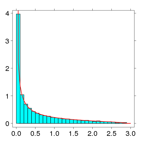
Figure 2 shows the asymptotic spectrum of $\mathbf{HH}^{\ast}$ against the corresponding matrix of size $1000\times 1000$ when the correlations $\{r_{k}^{2},t_{k}^{2}\}$ are assumed to obey the uniform distribution on $[0,1]$. The figure shows good agreement.

Figure 2: Histograms of the eigenvalues against the computed density.

Remark 5.

Other symmetric-like channels can also be solved using the above approach, for example

$$\mathbf{X}=\left(\begin{matrix}x_{1}&x_{2}&x_{3}\\ x_{3}&x_{1}&x_{2}\\ x_{2}&x_{3}&x_{1}\end{matrix}\right),\quad\quad\quad\mathbf{X}=\left(\begin{matrix}x_{1}&x_{4}&x_{5}\\ x_{4}&x_{2}&x_{6}\\ x_{5}&x_{6}&x_{3}\end{matrix}\right).$$

Observe that neither the matrix computed in this example nor the above matrices have a separable correlation matrix.

5 Comparison With Other Models

In order to compare the operator-valued Kronecker model with some of the classical models, in this section we compute the isotropic mutual information of a $2\times 2$ multiantenna system with Kronecker correlation given by

$$K:=\frac{1}{8}\left(\begin{matrix}1&0\\ 0&3\end{matrix}\right)\otimes\left(\begin{matrix}3&0\\ 0&5\end{matrix}\right),$$

the asymptotic isotropic mutual information predicted by the usual Kronecker correlation model, and the corresponding quantity based on the operator-valued model. For such a channel, one possibility for implementing the classical Kronecker correlation model is to take three noncommutative random variables $r$, $x$ and $t$ such that $x$ is circular and the distributions of $r^{2}$ and $t^{2}$ are given by

$$\mu_{r^{2}} =\frac{1}{2}\delta_{\frac{1}{2}}+\frac{1}{2}\delta_{\frac{3}{2}},$$

$$\mu_{t^{2}} =\frac{1}{2}\delta_{\frac{3}{4}}+\frac{1}{2}\delta_{\frac{5}{4}}.$$

From this it is clear that we may compute the asymptotic isotropic mutual information of the classical Kronecker model within the framework of the operator-valued Kronecker model. In particular, the classical Kronecker correlation model corresponds to the $n=1$ operator-valued Kronecker model. This shows that the operator-valued Kronecker model is a generalization of the usual Kronecker model also from this operational point of view.

The operator-valued Kronecker model uses $\Sigma^{2}=K$, but we have to use a model for the correlation produced by the asymptotic antenna patterns. Here we use two types of antenna pattern correlations. In one case we assume that the distribution of the correlation operators $\{r_{k},t_{k}\}$ take 1 with probability one, i.e., there is no correlation due to the antenna patterns; in the second case we assume that their distribution is given by

$$\mu=\frac{18}{38}\delta_{1}+\frac{12}{38}\delta_{\frac{1}{2}}+\frac{8}{38}\delta_{\frac{1}{4}}.$$ (8)

This distribution is motivated by an exponential decay law. In both cases we set $\gamma=1$.

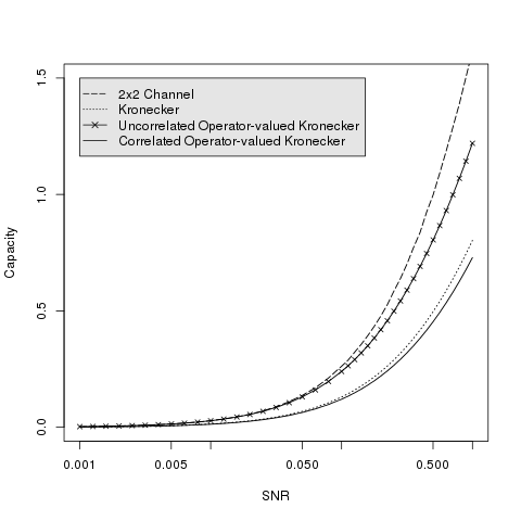
Figure 3 shows the mutual information of each model. The mutual information of the $2\times 2$ system was computed using a Monte Carlo simulation. From this figure, we observe that the highest mutual information is produced by the $2\times 2$ system. This is caused by the tail of the eigenvalue distribution of the $2\times 2$ random matrix involved. It is also important to notice that the operator-valued model predicts more mutual information than the usual Kronecker model when we assume no antenna pattern correlations. However, in the presence of antenna pattern correlations, the mutual information predicted by the operator-valued Kronecker model goes below the one predicted by the classical Kronecker model. In particular, this shows that the impact of the antenna design may be more significant than the impact of the propagation environment itself.

Figure 3: Isotropic mutual information predicted by the different models with respect to $P$.

Remark 6.

Observe that in this example the correlation satisfies the hypothesis of the previous section. In particular,

$$\scriptstyle\left(\begin{matrix}\sqrt{\frac{1}{2}}&0\\ 0&\sqrt{\frac{3}{2}}\end{matrix}\right)\left(\begin{matrix}x_{1}&x_{2}\\ x_{3}&x_{4}\end{matrix}\right)\left(\begin{matrix}\sqrt{\frac{3}{4}}&0\\ 0&\sqrt{\frac{5}{4}}\end{matrix}\right)=\left(\begin{matrix}\sqrt{\frac{3}{8}}x_{1}&0\\ 0&0\end{matrix}\right)+\left(\begin{matrix}0&\sqrt{\frac{5}{8}}x_{2}\\ 0&0\end{matrix}\right)+\left(\begin{matrix}0&0\\ \sqrt{\frac{9}{8}}x_{3}&0\end{matrix}\right)+\left(\begin{matrix}0&0\\ 0&\sqrt{\frac{15}{8}}x_{4}\end{matrix}\right).$$

This shows that the operator-valued Kronecker model may be used for some specific separable correlation channels.

Appendix A Prerequisites

A.1 Notation

$\mathbb{N}$: the set of natural numbers;

$\textnormal{M}_{n\times m}\left(\mathcal{C}\right)$: the set of all $n\times m$ matrices with entries from the algebra $\mathcal{C}$;

$A_{i,j}$ or $[A]_{i,j}$: the $i,j$th entry of the matrix $A$;

$A^{\top}$ the transpose of the matrix $A$, and $A^{\ast}$, its conjugate transpose;

$E_{i,j}$: the $i,j$-unit matrix in $\textnormal{M}_{n\times m}\left(\mathbb{C}\right)$;

$\mathrm{I}_{n}$: the identity matrix in $\textnormal{M}_{n}\left(\mathbb{C}\right)$;

$\mathbb{E}$:   expected valued with respect to a classical probability space $(\Omega,\mathcal{F},\mathbb{P})$;

A.2 Operator-Valued Free Probability Background

In what follows, $\mathcal{C}$ will denote a noncommutative unital $C^{\ast}$-algebra with unit $\mathbf{1}_{\mathcal{C}}$, and $\varphi:\mathcal{C}\rightarrow\mathbb{C}$ is a unit-preserving positive linear functional, i.e., $\varphi\left(\mathbf{1}_{\mathcal{C}}\right)=1$ and $\varphi\left(aa^{\ast}\right)\geq 0$ for any $a\in\mathcal{C}$. The pair $(\mathcal{C},\varphi)$ is called a noncommutative probability space and the elements of $\mathcal{C}$ are called noncommutative random variables. Unless otherwise stated, we use Greek letters to denote scalar numbers, lower case letters for noncommutative random variables in $\mathcal{C}$, upper case letters for matrices or random matrices in $\textnormal{M}_{n}\left(\mathbb{C}\right)$, and upper case bold letters for matrices in $\textnormal{M}_{n}\left(\mathcal{C}\right)$. The latter are called operator-valued matrices and $(\textnormal{M}_{n}\left(\mathcal{C}\right),\text{tr}_{n}\otimes\varphi)$ is a noncommutative probability space [12].

Given a selfadjoint element $a\in\mathcal{C}$, its algebraic distribution is the collection of its moments, i.e., $(\varphi\left(a^{k}\right))_{k\geq 1}$. Let $(\mathcal{A},\varphi)$ and $(\mathcal{A}_{n},\varphi_{n})$ for $n\geq 1$ be noncommutative probability spaces. If $a\in\mathcal{A}$ and $a_{n}\in\mathcal{A}_{n}$ for $n\geq 1$ are selfadjoint elements, we say that $(a_{n})_{n\geq 1}$ converges in distribution to $a$ as $n\rightarrow\infty$ if the corresponding moments converge, i.e.,

$$\lim_{n\rightarrow\infty}\varphi_{n}(a_{n}^{m})=\varphi\left(a^{m}\right)$$

for all $m\in\mathbb{N}$. If there is a probability measure $\mu$ in $\mathbb{C}$ with compact support such that for all $m\in\mathbb{N}$

$$\varphi\left(a^{m}\right)=\int_{\mathbb{C}}\zeta^{m}\,\mu(\mathrm{d}\zeta),$$

we call $\mu$ the analytical distribution of $a$. A family $a_{1},\ldots,a_{n}\in\mathcal{A}$ of noncommutative random variables is said to be free if

$$\varphi\left([p_{1}(a_{i_{1}})-\varphi\left(p_{1}(a_{i_{1}})\right)]\cdots[p_{k}(a_{i_{k}})-\varphi\left(p_{k}(a_{i_{k}})\right)]\right)=0$$

for all $k\in\mathbb{N}$, polynomials $p_{1},\ldots,p_{k}$ and $i_{1},\ldots,i_{k}\in\{1,\ldots,n\}$ such that $i_{l}\neq i_{l+1}$ for $1\leq l\leq k-1$. Let $A_{n}$ and $B_{n}$ be random matrices in $\textnormal{M}_{n}\left(\mathbb{C}\right)$ for every $n\geq 1$. If there exists $a,b\in\mathcal{C}$ such that $a$ and $b$ are free and $(A_{n},B_{n})$ converge in distribution to $(a,b)$, i.e.,

$$\lim_{n\rightarrow\infty}\frac{1}{n}\text{tr}\left(A_{n}^{l_{1}}B_{n}^{m_{1}}\cdots A_{n}^{l_{k}}B_{n}^{m_{k}}\right)=\varphi\left(a^{l_{1}}b^{m_{1}}\cdots a^{l_{k}}b^{m_{k}}\right)$$

for all $k,l_{1},\ldots,l_{k},m_{1},\ldots,m_{k}\in\mathbb{N}$, we say that $A_{n}$ and $B_{n}$ are asymptotically free.

Given a probability measure $\mu$ in $\mathbb{R}$, its (scalar) Cauchy transform $G_{\mu}:\mathbb{C}^{+}\rightarrow\mathbb{C}^{-}$ is defined as

$$G_{\mu}(\zeta):=\int_{\mathbb{R}}\frac{\mu(\text{d}\xi)}{\zeta-\xi}.$$

The Stieltjes inversion formula states that if $\mu$ has density $f:\mathbb{R}\rightarrow\mathbb{R}$ then

$$f(\xi)=-\frac{1}{\pi}\lim_{\begin{smallmatrix}\zeta\in\mathbb{R}\\ \zeta\rightarrow 0+\end{smallmatrix}}\Im(G_{\mu}(\xi+i\zeta))$$

for all $\xi\in\mathbb{R}$, where $\Im$ denotes the imaginary part and $\Re$ the real part.

Let $\mathcal{H}^{+}(\textnormal{M}_{n}\left(\mathbb{C}\right))\subset\textnormal{M}_{n}\left(\mathbb{C}\right)$ denote the set of matrices $B$ such that $\Im(B):=\dfrac{B-B^{\ast}}{2i}$ is positive definite, and define $\mathcal{H}^{-}(\textnormal{M}_{n}\left(\mathbb{C}\right)):=-\mathcal{H}^{+}(\textnormal{M}_{n}\left(\mathbb{C}\right))$. For an operator-valued matrix $\mathbf{X}\in\textnormal{M}_{n}\left(\mathcal{C}\right)$ we define its $\textnormal{M}_{n}\left(\mathbb{C}\right)$-valued Cauchy transform $G_{\mathbf{X}}:\mathcal{H}^{+}(\textnormal{M}_{n}\left(\mathbb{C}\right))\rightarrow\mathcal{H}^{-}(\textnormal{M}_{n}\left(\mathbb{C}\right))$ by

$$G_{\mathbf{X}}(B) =E\left((B-\mathbf{X})^{-1}\right)$$ (9)

$$=\sum_{n\geq 0}B^{-1}E\left((\mathbf{X}B^{-1})^{n}\right),$$

where the last power series converges in a neighborhood of infinity. The scalar Cauchy transform of $\mathbf{X}$ is given by

$$G(\zeta)=\text{tr}_{n}(G_{\mathbf{X}}(\zeta\mathrm{I}_{n}))\mathbf{,\quad}\zeta\in\mathbb{C}\mathbf{.}$$ (10)

The freeness relation over $\textnormal{M}_{n}\left(\mathbb{C}\right)$ is defined similarly to the usual freeness, but taking $E$ instead of $\varphi$ and non-commutative polynomials over $\textnormal{M}_{n}\left(\mathbb{C}\right)$ instead of complex polynomials. The main tools that we use from the subordination theory are the following formulas to compute the $\textnormal{M}_{n}\left(\mathbb{C}\right)$-valued Cauchy transforms of sums and products of free elements in $\textnormal{M}_{n}\left(\mathcal{C}\right)$; see [3, 4].

If $\mathbf{X}=\mathbf{X}^{\ast}$ is an operator-valued matrix in $\textnormal{M}_{n}\left(\mathcal{C}\right)$, we define the $r_{\mathbf{X}}$ and $h_{\mathbf{X}}$ transforms, for $B\in\mathcal{H}^{+}(\textnormal{M}_{n}\left(\mathbb{C}\right))$, by

$$r_{\mathbf{X}}(B) =G_{\mathbf{X}}(B)^{-1}-B,$$

$$h_{\mathbf{X}}(B) =B^{-1}-G_{\mathbf{X}}(B^{-1})^{-1}.$$

Theorem 5.

Let $\mathbf{X},\mathbf{Y}\in\textnormal{M}_{n}\left(\mathcal{C}\right)$ be selfadjoint elements free over $\textnormal{M}_{n}\left(\mathcal{C}\right)$.

i) For all $B\in\mathcal{H}^{+}(\textnormal{M}_{n}\left(\mathbb{C}\right))$, we have that

$$G_{\mathbf{X}+\mathbf{Y}}{B}=G_{\mathbf{X}}(\omega_{1}(B)),$$ (11)

where $\omega_{1}(B)=\lim_{n\rightarrow\infty}f_{B}^{n}(W)$ for any $W\in\mathcal{H}^{+}(\textnormal{M}_{n}\left(\mathcal{C}\right))$ and

$$f_{b}(W)=r_{\mathbf{Y}}(r_{\mathbf{X}}(W)+B)+B.$$

ii) In addition, if $\mathbf{X}$ is positive definite, $E\left(\mathbf{X}\right)$ and $E\left(\mathbf{Y}\right)$ invertible, and we define for all $B\in\mathcal{H}^{+}(\textnormal{M}_{n}\left(\mathbb{C}\right))$ with $\Im(B\mathbf{X})>0$ the function $g_{B}(W)=Bh_{\mathbf{X}}(h_{\mathbf{Y}}(W)B)$ for all $W\in\mathcal{H}^{+}(\textnormal{M}_{n}\left(\mathbb{C}\right))$, then there exists a function $\omega_{2}$ such that

$$\omega_{2}(B)=\lim_{n\rightarrow\infty}g_{B}^{n}(W)$$

for all $W\in\mathcal{H}^{+}(\textnormal{M}_{n}\left(\mathbb{C}\right))$, and

$$G_{\mathbf{XY}}(z\mathrm{I}_{n}) =(z\mathrm{I}_{n}-h_{\mathbf{XY}}(z^{-1}\mathrm{I}_{n}))^{-1},$$ (12)

$$zh_{\mathbf{XY}}(z\mathrm{I}_{n}) =\omega_{2}(z\mathrm{I}_{n})h_{\mathbf{Y}}(\omega_{2}(z\mathrm{I}_{n}))).$$

The functions above are defined in $\mathcal{H}^{+}(\textnormal{M}_{n}\left(\mathbb{C}\right))$. Whenever we evaluate any of these functions in $B\in\mathcal{H}^{-}(\textnormal{M}_{n}\left(\mathbb{C}\right))$ we have to do so by means of the relation $f(B)=f(B^{\ast})^{\ast}$.

Appendix B Proof of Theorem 1 and Further Analysis

B.1 Case $\gamma\to\infty$

It is a well known result [13] that the eigenvalues are continuous functions of the entries of a selfadjoint matrix. If the entries of a matrix $M$ lie in the unit circle, then its Frobenius norm is bounded and so its operator norm. In particular, $g(M):=(\lambda_{1}(MM^{*}),\ldots,\lambda_{N}(MM^{*}))$ is a bounded and continuous function of the entries of $M$. Therefore, if we prove that the entries of $A$ converge in distribution to the entries of $U$, i.e. $(A_{i,j})_{i,j=1}^{N}\overset{\textnormal{d}}{\to}(U_{i,j})_{i,j=1}^{N}$, then $g(A)\overset{\textnormal{d}}{\to}g(U)$ as required.

The entries of $A$ and $U$ lie in the unit circle, so we are dealing with compact support distributions. Thus, it is enough to show the convergence of the joint moments of the entries of $A$ to those of $U$ to ensure the multivariate convergence in distribution, and so the claimed convergence in the first part of Theorem 1.

Let $N\in\mathbb{N}$ be fixed, for $(n_{k,l})_{k,l=1}^{N}\subset\mathbb{Z}$

$$\mathbb{E}\left(\prod_{k,l=1}^{N}A_{k,l}^{n_{k,l}}\right) =\mathbb{E}\left(\prod_{k,l=1}^{N}\exp\left(\mathrm{i}\gamma n_{k,l}\theta_{k,l}\right)\right)$$

$$=\mathbb{E}\left(\prod_{k,l=1}^{N}\exp\left(\mathrm{i}\gamma n_{k,l}\sum_{i,j=1}^{N}R_{k,i}X_{i,j}T_{j,l}\right)\right)$$

$$=\mathbb{E}\left(\exp\left(\sum_{i,j=1}^{N}\mathrm{i}\gamma\left(\sum_{k,l=1}^{N}n_{k,l}R_{k,i}T_{j,l}\right)X_{i,j}\right)\right)$$

$$=\mathbb{E}\left(\prod_{i,j=1}^{N}\exp\left(\mathrm{i}\gamma\left(\sum_{k,l=1}^{N}n_{k,l}R_{k,i}T_{j,l}\right)X_{i,j}\right)\right)$$

$$=\prod_{i,j=1}^{N}\exp\left(-\frac{\gamma^{2}}{2}\left(\sum_{k,l=1}^{N}n_{k,l}R_{k,i}T_{j,l}\right)^{2}\right).$$

Since $R$ and $T$ are full rank, a linear algebra argument shows that the previous exponents are all zero if and only if $(n_{k,l})_{k,l=1}^{N}$ are all zero. Therefore, the joint moments of the entries of $A$ vanish as $\gamma\rightarrow\infty$ except when $n_{k,l}=0$ for all $k$ and $l$. It is easy to show that these limiting moments are indeed the joint moments of the entries of $U$. This conclude the proof of the first part.

B.2 Case $\gamma\to 0$

The following lemma and two theorems are from Appendix A in [1]

Lemma 1.

Let $A_{1},\ldots,A_{l}\in\textnormal{M}_{m\times n}\left(\mathbb{C}\right)$. Then

$$\left|\left|A_{1}\circ A_{2}\circ\cdots\circ A_{l}\right|\right|\leq\left|\left|A_{1}\right|\right|\left|\left|A_{2}\right|\right|\cdots\left|\left|A_{l}\right|\right|,$$

where $A\circ B$ denotes the pointwise or Hadamard product of $A$ and $B$.

Theorem 6.

Let $A,B\in\textnormal{M}_{m\times n}\left(\mathbb{C}\right)$. Then

$$\sum_{k=1}^{p}|\sigma_{k}(A)-\sigma_{k}(B)|^{2}\leq\text{tr}\left((A-B)(A-B)^{*}\right)$$

where $p=\min(m,n)$ and $\sigma_{1}(\cdot)\geq\cdots\geq\sigma_{p}(\cdot)$ are the singular values of $\cdot$.

Theorem 7.

Let $A$ and $B$ be two $m\times n$ complex matrices. Then, for any Hermitian complex matrices $X\in\textnormal{M}_{m}\left(\mathbb{C}\right)$ and $Y\in\textnormal{M}_{n}\left(\mathbb{C}\right)$ we have that

$$||F^{X+AYA^{*}}-F^{X+BYB^{*}}||\leq\frac{1}{m}\textnormal{rank}\left(A-B\right).$$

In this rest of this subsection, $F^{A}$ will denote the empirical distribution of the singular values $\sigma_{1}(A)\geq\cdots\geq\sigma_{n}(A)$ of $A\in\textnormal{M}_{n\times n}\left(\mathbb{C}\right)$. Since the classical convergence theorems in random matrices hold almost surely, it is enough to deal with the case of non-random matrices.

Lemma 2.

Let $A,B\in\textnormal{M}_{N}\left(\mathbb{C}\right)$. Then

$$\sum_{k=1}^{N}|\sigma_{k}(A)-\sigma_{k}(B)|\leq\sqrt{N\text{tr}\left((A-B)(A-B)^{*}\right)}.$$

Proof.

An straightforward application of Theorem 6 and the generalized means. ∎

Definition 1.

We define the entrywise exponential function $\exp_{\circ}:\textnormal{M}_{m\times n}\left(\mathbb{C}\right)\to\textnormal{M}_{m\times n}\left(\mathbb{C}\right)$ by

$$\exp_{\circ}(A)=(\exp(A_{i,j}))_{i,j}$$

for all $A\in\textnormal{M}_{m\times n}\left(\mathbb{C}\right)$.

Proposition 1.

Let $A\in\textnormal{M}_{N}\left(\mathbb{C}\right)$ for $N\in\mathbb{N}$ and $1>\gamma>0$. Let $X=\exp_{\circ}(i\gamma A)$, then

$$\frac{1}{N}\sum_{k=2}^{N}\left|\sigma_{k}\left(\frac{X}{\gamma}\right)-\sigma_{k}(A)\right|\leq\gamma\exp(\left|\left|A\right|\right|)+\frac{2||A||}{N}.$$ (13)

Proof.

Using the power series for the exponential function we obtain that

$$X={\bf 1}_{N}+i\gamma A+\sum_{n\geq 2}\frac{(i\gamma A)^{\circ n}}{n!}$$ (14)

where $T^{\circ n}=T\circ T\circ\cdots\circ T$. Define $Z={\bf 1}_{N}+i\gamma A$ and $Y=X-Z$. By Lemma 1 and the fact that $\gamma<1$,

$$\left|\left|Y\right|\right| =\gamma^{2}\left|\left|\sum_{n\geq 2}\gamma^{n-2}\frac{(iA)^{\circ n}}{n!}\right|\right|$$

$$\leq\gamma^{2}\exp(\left|\left|A\right|\right|).$$

By Lemma 2 we have that

$$\sum_{k=1}^{N}\left|\sigma_{k}(X)-\sigma_{k}(Z)\right| \leq\sqrt{N\textrm{tr}\left(YY^{*}\right)}$$

$$\leq\sqrt{N^{2}\left|\left|Y\right|\right|^{2}}$$

$$\leq\gamma^{2}N\exp(\left|\left|A\right|\right|)$$ (15)

and in particular

$$\frac{1}{N}\sum_{k=2}^{N}\left|\sigma_{k}\left(\frac{X}{\gamma}\right)-\sigma_{k}\left(\frac{Z}{\gamma}\right)\right|\leq\gamma\exp(\left|\left|A\right|\right|).$$ (16)

Applying Theorem 7 to the matrices $Z$ and $\gamma A$ we obtain

$$\left|\left|F^{ZZ^{*}}-F^{AA^{*}}\right|\right|\leq\frac{1}{N}\textnormal{rank}\left({\bf 1}_{N}\right)=\frac{1}{N},$$

which implies that

$$\left|\sum_{k=1}^{N}1_{x\leq\sigma_{k}(Z)^{2}}-\sum_{k=1}^{N}1_{x\leq\sigma_{k}(\gamma A)^{2}}\right|\leq 1$$

for all $x\in\mathbb{R}$. This implies that for $2\leq k\leq N-1$

$$\sigma_{k+1}(\gamma A)\leq\sigma_{k}(Z)\leq\sigma_{k-1}(\gamma A),$$ (17)

and equivalently

$$\sigma_{k+1}(\gamma A)-\sigma_{k}(\gamma A)\leq\sigma_{k}(Z)-\sigma_{k}(\gamma A)\leq\sigma_{k-1}(\gamma A)-\sigma_{k}(\gamma A).$$

Therefore

$$|\sigma_{k}(Z)-\sigma_{k}(\gamma A)| \leq\sigma_{k-1}(\gamma A)-\sigma_{k}(\gamma A)+\sigma_{k}(\gamma A)-\sigma_{k+1}(\gamma A)$$

$$=\sigma_{k-1}(\gamma A)-\sigma_{k+1}(\gamma A),$$

and consequently

$$\sum_{k=2}^{N}|\sigma_{k}(Z)-\sigma_{k}(\gamma A)| \leq\sum_{k=2}^{N-1}\sigma_{k-1}(\gamma A)-\sigma_{k+1}(\gamma A)+|\sigma_{N}(Z)-\sigma_{N}(\gamma A)|$$

$$\leq\sigma_{1}(\gamma A)+\sigma_{2}(\gamma A)-\sigma_{N-1}(\gamma A)-\sigma_{N}(\gamma A)+\sigma_{N}(Z)+\sigma_{N}(\gamma A).$$

Using the same argument that in equation (17) we have that $\sigma_{N}(Z)\leq\sigma_{N-1}(\gamma A)$ and thus

$$\sum_{k=2}^{N}|\sigma_{k}(Z)-\sigma_{k}(\gamma A)|\leq 2\gamma||A||$$

and in particular

$$\frac{1}{N}\sum_{k=2}^{N}\left|\sigma_{k}\left(\frac{Z}{\gamma}\right)-\sigma_{k}(A)\right|\leq\frac{2||A||}{N}.$$

By the triangle inequality we conclude that

$$\frac{1}{N}\sum_{k=2}^{N}\left|\sigma_{k}\left(\frac{X}{\gamma}\right)-\sigma_{k}(A)\right|\leq\gamma\exp(\left|\left|A\right|\right|)+\frac{2||A||}{N}$$

as claimed. ∎

Observe that the previous analysis exclude the biggest singular value of $X/\sigma$. In the following proposition we study the behavior of this singular value.

Proposition 2.

In the notation of the previous proposition,

$$\left|\frac{\sigma_{1}(X/\gamma)}{N/\gamma}-1\right|\leq\gamma(\gamma\exp(\left|\left|A\right|\right|)+\left|\left|A\right|\right|).$$

This shows that $\sigma_{1}(X/\gamma)$ is roughly $N/\gamma$, while the bulk of $X/\gamma$ is essentially the same as $A$.

Proof.

By inequality (15) in the first part of the previous proof

$$\left|\sigma_{1}\left(\frac{X}{\gamma}\right)-\sigma_{1}\left(\frac{Z}{\gamma}\right)\right|\leq\gamma N\exp(\left|\left|A\right|\right|).$$ (18)

Using Lemma 2 for $Z/\gamma$ and ${\bf 1}_{N}/\gamma$

$$\left|\sigma_{1}\left(\frac{Z}{\gamma}\right)-\sigma_{1}\left(\frac{{\bf 1}_{N}}{\gamma}\right)\right| \leq\sqrt{N\textrm{tr}\left(AA^{*}\right)}$$

$$\leq N\left|\left|A\right|\right|.$$

A straightforward computation shows that $\sigma_{1}({\bf 1}_{N}/\gamma)=N/\gamma$, so by the triangle inequality

$$\left|\frac{\sigma_{1}(X/\gamma)}{N/\gamma}-1\right|\leq\gamma(\gamma\exp(\left|\left|A\right|\right|)+\left|\left|A\right|\right|),$$

as claimed. ∎

Finally, with the previous quantitative results we prove the following qualitative result.

Theorem 8.

Let $A_{N}\in\textnormal{M}_{N}\left(\mathbb{C}\right)$ such that $\left|\left|A_{N}\right|\right|$ converge as $N\to\infty$ and $F^{A_{N}}\Rightarrow F^{A}$. Define $X_{N}=\exp_{\circ}(i\gamma_{N}A_{N})$. If $(\gamma_{N})_{N\geq 1}$ is a sequence of positive real numbers such that $\gamma_{N}\to 0$ as $N\to\infty$, then $F^{X_{N}/\gamma_{N}}\Rightarrow F^{A}$ as $N\to\infty$.

Proof.

Recall that $F^{X_{N}/\gamma_{N}}\Rightarrow F^{A}$ if and only if

$$\lim_{N\to\infty}\int_{\mathbb{R}}f(x)\textrm{d}F^{X_{N}/\gamma_{N}}(x)=\int_{\mathbb{R}}f(x)\textrm{d}F^{A}(x)$$

for all $f$ bounded Lipschitz function. Let $f$ be any bounded Lipschitz function, by the previous propositions

$$\bigg{|}\int_{\mathbb{R}}f(x)\textrm{d}F^{X_{N}/\gamma_{N}}(x) -\int_{\mathbb{R}}f(x)\textrm{d}F^{A_{N}}(x)\bigg{|}$$

$$=\left|\frac{1}{N}\sum_{k=1}^{N}f\left(\sigma_{k}\left(\frac{X_{N}}{\gamma_{N}}\right)\right)-\frac{1}{N}\sum_{k=1}^{N}f(\sigma_{k}(A_{N}))\right|$$

$$\leq\frac{1}{N}\sum_{k=1}^{N}\left|f\left(\sigma_{k}\left(\frac{X_{N}}{\gamma_{N}}\right)\right)-f(\sigma_{k}(A_{N}))\right|$$

$$\leq\frac{K}{N}\sum_{k=2}^{N}\left|\sigma_{k}\left(\frac{X_{N}}{\gamma_{N}}\right)-\sigma_{k}(A_{N})\right|+\frac{\left|f\left(\sigma_{1}\left(\frac{X_{N}}{\gamma_{N}}\right)\right)\right|+|f(\sigma_{1}(A_{N}))|}{N},$$

where $K$ is the Lipschitz constant of $f$. Since $f$ is bounded and $\left|\left|A_{N}\right|\right|$ converge as $N\to\infty$, by Proposition 1 the previous expression converges to 0 as $N\to\infty$. Finally, since $F^{A_{N}}\Rightarrow F^{A}$ as $N\to\infty$ we have that

$$\lim_{N\to\infty}\left|\int_{\mathbb{R}}f(x)\textrm{d}F^{A_{N}}(x)-\int_{\mathbb{R}}f(x)\textrm{d}F^{A}(x)\right|=0$$

and by the triangle inequality the result follows. ∎

The second part of Theorem 1 is an straightforward application of the previous theorem.

Appendix C Computation of Some Cauchy Transforms

Proof of Theorem 2. The identities $E_{k,k}BE_{k,k}=B_{k,k}E_{k,k}$ and $E_{k,k}^{2}=E_{k,k}$ lead to

$$G_{r_{k}^{2}E_{k,k}}(B) =\sum_{n\geq 0}B^{-1}E\left((r_{k}^{2}E_{k,k}B^{-1})^{n}\right)$$

$$=B^{-1}+B^{-1}\sum_{n\geq 1}\varphi\left(r_{k}^{2n}\right)[B^{-1}]_{k,k}^{n-1}E_{k,k}B^{-1}$$

$$=B^{-1}+[B^{-1}]_{k,k}^{-2}\left(\sum_{n\geq 0}\varphi\left(r_{k}^{2n}\right)[B^{-1}]_{k,k}^{n+1}-[B^{-1}]_{k,k}\right)B^{-1}E_{k,k}B^{-1}$$

$$=B^{-1}+[B^{-1}]_{k,k}^{-2}\left(G_{r_{k}^{2}}([B^{-1}]_{k,k}^{-1})-[B^{-1}]_{k,k}\right)B^{-1}E_{k,k}B^{-1}.$$

Of course, the previous equations do not hold for every matrix $B\in\textnormal{M}_{2n}\left(\mathbb{C}\right)$, in particular, the power series expansion is valid only in a neighborhood of infinity. However, the previous computation can be carried out at the level of formal power series, and then extended via analytical continuation to a suitable domain.

Proof of Theorem 3. A straightforward computation shows that

$$G_{\mathbf{Q}}(D) =\sum_{k\geq 0}D^{-1}E\left((\mathbf{Q}D^{-1})^{k}\right)$$

$$=\sum_{k\geq 0}\textnormal{diag}\left(d_{1}^{-1},\ldots,d_{2n}^{-1}\right)E\left(\textnormal{diag}\left(d_{1}^{-k}r_{1}^{k},\ldots,d_{n}^{-k}r_{n}^{k},d_{n+1}^{-k}t_{1}^{k},\cdots,d_{2n}^{-k}t_{n}^{k}\right)\right)$$

$$=\sum_{k\geq 0}\textnormal{diag}\left(d_{1}^{-(k+1)}\varphi\left(r_{1}^{k}\right),\ldots,d_{2n}^{-(k+1)}\varphi\left(t_{n}^{k}\right)\right)$$

$$=\textnormal{diag}\left(G_{r_{1}}(d_{1}),\ldots,G_{t_{n}}(d_{2n})\right).$$

Proof of Theorem 4. Observe that

$$\widehat{Mx}J^{-1}=\left(\begin{matrix}0&DPx\\ (DP)^{\ast}x^{\ast}&0\end{matrix}\right)\left(\begin{matrix}J_{1}^{-1}&0\\ 0&J_{2}^{-1}\end{matrix}\right)=\left(\begin{matrix}0&DPJ_{2}^{-1}x\\ (DP)^{\ast}J_{1}^{-1}x^{\ast}&0\end{matrix}\right).$$

Thus,

$$\left(\widehat{Mx}J^{-1}\right)^{2}=\left(\begin{matrix}DPJ_{2}^{-1}(DP)^{\ast}J_{1}^{-1}xx^{\ast}&0\\ 0&(DP)^{\ast}J_{1}^{-1}DPJ_{2}^{-1}x^{\ast}x\end{matrix}\right).$$

Since $P^{\top}D^{\prime}P$ and $PD^{\prime}P^{\top}$ are diagonal for any diagonal matrix $D^{\prime}$, and diagonal matrices commute, we have for $n\geq 1$ that

$$\left(\widehat{Mx}J^{-1}\right)^{2n}=\left(\begin{matrix}J_{1}^{-n}(DPJ_{2}^{-1}(DP)^{\ast})^{n}(xx^{\ast})^{n}&0\\ 0&((DP)^{\ast}J_{1}^{-1}DP)^{n}J_{2}^{-n}(x^{\ast}x)^{n}\end{matrix}\right).$$

Recalling that the odd moments of $x$ are zero, the previous equation implies

$$G_{\widehat{Mx}}(J) =\sum_{n\geq 0}J^{-1}E\left(\left(\widehat{Mx}J^{-1}\right)^{n}\right)$$

$$=\sum_{n\geq 0}J^{-1}E\left(\left(\widehat{Mx}J^{-1}\right)^{2n}\right)$$

$$=\sum_{n\geq 0}\left(\begin{matrix}J_{1}^{-(n+1)}(DPJ_{2}^{-1}(DP)^{\ast})^{n}\varphi\left((xx^{\ast})^{n}\right)&0\\ 0&((DP)^{\ast}J_{1}^{-1}DP)^{n}J_{2}^{-(n+1)}\varphi\left((x^{\ast}x)^{n}\right)\end{matrix}\right).$$

Finally, let $\pi$ be the permutation associated to $P$, then $[PD^{\prime}]_{k}=[D^{\prime}]_{\pi(k)}$ for any diagonal matrix $D^{\prime}$ and any $1\leq k\leq n$. Therefore

$$G_{\widehat{Mx}}(J) =\left(\begin{matrix}(DPJ_{2}^{-1}(DP)^{\ast})^{-1}&0\\ 0&((DP)^{\ast}J_{1}^{-1}DP)^{-1}\end{matrix}\right)\times$$

$$\quad\quad\sum_{n\geq 0}\left(\begin{matrix}J_{1}^{-(n+1)}(DPJ_{2}^{-1}(DP)^{\ast})^{n+1}\varphi\left((xx^{\ast})^{n}\right)&0\\ 0&((DP)^{\ast}J_{1}^{-1}DP)^{n+1}J_{2}^{-(n+1)}\varphi\left((x^{\ast}x)^{n}\right)\end{matrix}\right)$$

$$=\left(\begin{matrix}(DPJ_{2}^{-1}(DP)^{\ast})^{-1}&0\\ 0&((DP)^{\ast}J_{1}^{-1}DP)^{-1}\end{matrix}\right)\times$$

$$\quad\quad\textnormal{diag}\left(G_{xx^{\ast}}([J_{1}]_{1}[J_{2}]_{\pi(1)}|D_{1}|^{-2}),\ldots,G_{x^{\ast}x}([J_{1}]_{\pi^{-1}(n)}[J_{2}]_{n}|D_{\pi^{-1}(n)}|^{-2})\right)$$

$$=\mathrm{diag}([J_{2}]_{\pi(1)}|D_{1}|^{-2}G_{xx^{\ast}}([J_{1}]_{1}[J_{2}]_{\pi(1)}|D_{1}|^{-2}),\ldots$$

$$\quad\quad\ldots,[J_{1}]_{\pi^{-1}(n)}|D_{\pi^{-1}(n)}|^{-2}G_{x^{\ast}x}([J_{1}]_{\pi^{-1}(n)}[J_{2}]_{n}|D_{\pi^{-1}(n)}|^{-2})).$$

References

- [1] Bai, Z. and Silverstein, J. (2010). Spectral Analysis of Large Dimensional Random Matrices. Springer, United States.
- [2] Benaych-Georges, F. (2009). Rectangular random matrices, related free entropy and free Fisher’s information. J. Operator Theory 62, 371–419.
- [3] Belinschi, S., Mai, T. and Speicher, R. (2013). Analytic subordination theory of operator-valued free additive convolution and the solution of a general random matrix problem. arXiv:1303.3196.
- [4] Belinschi, S., Speicher, R., Treilhard, J. and Vargas, C. (2012). Operator-valued free multiplicative convolution: Analytic subordination theory and applications to random matrix theory. arXiv:1209.3508.
- [5] Coulliet, R. and Debbah, M. (2011). Random Matrix Methods for Wireless Communications. Cambridge University Press, United Kingdom.
- [6] Far, R., Oraby, T., Bryc W. and Speicher R. (2008). On slow-fading MIMO systems with nonseparable correlation. IEEE Trans. on Information Theory 54, 544–553.
- [7] Fonollosa, J., Mestre X. and Pagès-Zamora, A. (2003). Capacity of MIMO channels: Asymptotic evaluation under correlated fading. IEEE Journal on Selected Areas in Communications 21, 829–838.
- [8] Foschini, G., Gans, M., Kahn, J. and Shiu, D. (2000). Fading Correlation and Its Effects on the Capacity of Multielement Antenna Systems. IEEE Trans. on Communications 48, 502–513.
- [9] Hiai, F. and Petz, D. (2000). The Semicircle Law, Free Random Variables and Entropy. American Mathematical Society, United States.
- [10] Nica, A. and Speicher, R. (2006). Lectures on the Combinatorics of Free Probability. Cambridge University Press, United Kingdom.
- [11] Shlyakhtenko, D. (1996) Random Gaussian band matrices and freeness with amalgamation. Int Math Res Notices 1996, 1013–1025.
- [12] Speicher, R., Vargas, C. and Mai, T. (2012). Free deterministic equivalents, rectangular random matrix models and operator-valued free probability theory. Random Matrices: Theory and Applications 1.
- [13] Tao, T. (2012). Topics in Random Matrix Theory. American Mathematical Society, United States.
- [14] Telatar, E. (1999). Capacity of multi-antenna Gaussian channels. Euro. Trans. Telecommunications 10, 585–595.
- [15] Tulino, A., Lozano, A. and Verdú, S. (2005). Impact of antenna correlation on the capacity of multiantenna channels. IEEE Trans. on Information Theory 51, 2491–2509.