HAT-P-54b: A Hot Jupiter Transiting a $0.64$ $M_{\sun}$ Star in Field 0 of the K2 Mission

Abstract

We report the discovery of HAT-P-54b, a planet transiting a late K dwarf star in field 0 of the NASA K2 mission. We combine ground-based photometric light curves with radial velocity measurements to determine the physical parameters of the system. HAT-P-54b has a mass of $0.760\pm 0.032$ $M_{\rm J}$, a radius of $0.944\pm 0.028$ $R_{\rm J}$, and an orbital period of $3.7998$ d. The star has $V=13.505\pm 0.060$, a mass of $0.645\pm 0.020$ $M_{\sun}$, a radius of $0.617\pm 0.013$ $R_{\sun}$, an effective temperature of $T_{\rm eff\star}=4390\pm 50$, and a subsolar metallicity of $\rm[Fe/H]=-0.127\pm 0.080$. HAT-P-54b has a radius that is smaller than 92% of the known transiting planets with masses greater than that of Saturn, while HAT-P-54 is one of the lowest-mass stars known to host a hot Jupiter. Follow-up high-precision photometric observations by the K2 mission promise to make this a well-studied planetary system.

1. Introduction

Among the best studied transiting planets are the three planets discovered by wide-field ground-based surveys in the field of the NASA Kepler mission prior to the mission launch. These planets, including TrES-2b (O’Donovan et al., 2006), HAT-P-7b (Pál et al., 2008) and HAT-P-11b (Bakos et al., 2010) orbit bright stars, have relatively deep transits, and have short orbital periods. These same factors enabled their discovery from the ground. The extremely high S/N ratio transit observations by Kepler have allowed a number of subtle effects to be studied for TrES-2b and HAT-P-7b. These include the optical phase variation and secondary eclipse due to reflected light from the planet, the tidal distortion of the star due to the planet, Doppler beaming, and the detection of p-mode oscillations enabling asteroseismology of the host stars, among others (Morris et al., 2013; Barclay et al., 2012; Jackson et al., 2012; Kipping & Bakos, 2011; Welsh et al., 2010; Borucki et al., 2009). For HAT-P-11b observations of starspot crossings by the planet have revealed the presence of active latitudes on the star, have been used to show that there is a high inclination between the spin axis of the star and the orbital axis of the planet (Sanchis-Ojeda & Winn, 2011; Deming et al., 2011), and have also revealed an apparent commensurability between the orbital period of the planet and the rotation period of the star (Béky et al., 2014). While the transits of these three systems could have easily been discovered from the Kepler light curves themselves, the prior ground-based detections ensured that the targets would be included among the limited number of stars for which data are downloaded, they extended the time base-line over which transits have been measured, and they provided a set of confirmed planets, including radial velocities (RVs) used to determine their masses, for which the performance of Kepler could be ascertained immediately after launch.

Following the failure of two of the Kepler reaction wheels, a repurposed Kepler mission, dubbed K2, has been proposed (Howell et al., 2014). In this mission the Kepler space telescope will be used to observe 10 fields along the ecliptic plane over the course of two years. Due to various constraints the number of stars that can be observed in each field is substantially lower than the number for the original Kepler mission. In this case prior observations of the K2 fields by ground-based telescopes to preselect targets are extremely valuable.

In this paper we present the discovery of a transiting planet, HAT-P-54b, in the first field that is observed by the K2 mission (called field 0). This planet, discovered by the HATNet survey (Bakos et al., 2004), is the first transiting planet to be identified in this field.

In Section 2 we summarize the detection of the photometric transit signal and the subsequent spectroscopic and photometric observations of the star to confirm the planet. In Section 3 we analyze the data to rule out false positive scenarios, and to determine the stellar and planetary parameters. We discuss our findings briefly in Section 4.

2. Observations

2.1. Photometry

2.1.1 Photometric detection

Photometric observations of the star HAT-P-54 (see identifying information in Table 3) were carried out by the fully automated HATNet system (Bakos et al., 2004) between 2011 Oct and 2012 May using the HAT-6 instrument at Fred Lawrence Whipple Observatory (FLWO) in Arizona, and between 2011 Oct and 2012 Feb using the HAT-9 instrument at Mauna Kea Observatory (MKO) in Hawaii. A total of 6609 images yielding acceptable photometry were obtained with HAT-6, and 4233 images with HAT-9. We used an exposure time of 180 s (median cadence of 214 s) and a Sloan $r$-band filter for the observations. Data were reduced to trend-filtered light curves following Bakos et al. (2010). The trend filtering included de-correlating the light curves against a set of measured parameters (which we refer to as External Parameter Decorrelation; or EPD), followed by application of the Trend Filtering Algorithm (TFA; Kovács et al., 2005). The per-point RMS scatter of the resulting light curves is 23.6 mmag for HAT-6 and 20.4 mmag for HAT-9, and is dominated by shot noise from the sky background.

Transits were detected in the combined light curve using the Box-fitting Least Squares algorithm (BLS; Kovács et al., 2002). The trend-filtered, phase-folded, combined light curve for HAT-P-54 is shown in Figure 1, while the individual photometric measurements are provided in Table 2.1.2.

We used BLS to search for additional transiting signals in the residual HATNet light curve (after subtracting the transits of HAT-P-54b) but found nothing significant above the noise. However, we found a significant sinusoidal variation most likely due to stellar activity (i.e., modulation of the brightness due to spots rotating on the surface of the star; see Section 3.3 for details).

In the following subsections we discuss the observations used to confirm HAT-P-54b as a transiting planet.

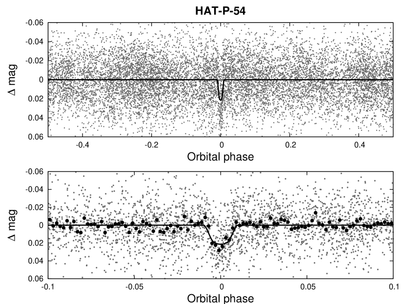
Figure 1.— HATNet light curve of HAT-P-54 phase folded with the transit period. The top panel shows the unbinned light curve, while the bottom shows the region zoomed-in on the transit, with dark filled circles for the light curve binned in phase with a binsize of 0.002. The solid line shows the model fit to the light curve.

2.1.2 Photometric follow-up

Higher precision photometric time series observations were obtained using the Keplercam imager on the FLWO 1.2 m telescope. We observed an egress on the night of 2012 Dec 6, and a full transit on the night of 2013 Jan 17. A total of 72 observations were made on the first night, and 87 were made on the second night. In both cases we used a Sloan $i$-band filter, and an exposure time of 150 s (yielding a median cadence of 165 s). The images were reduced to light curves following Bakos et al. (2010). We corrected the light curves for systematic variations using the EPD and TFA procedures as part of our model fitting procedure (Section 3). Figure 2 shows the resulting trend-filtered light curves, together with our best fit transiting planet light curve model. The data are provided in Table 2.1.2. The residuals from the best-fit model have a per-point RMS scatter of 0.9 mmag on each night.

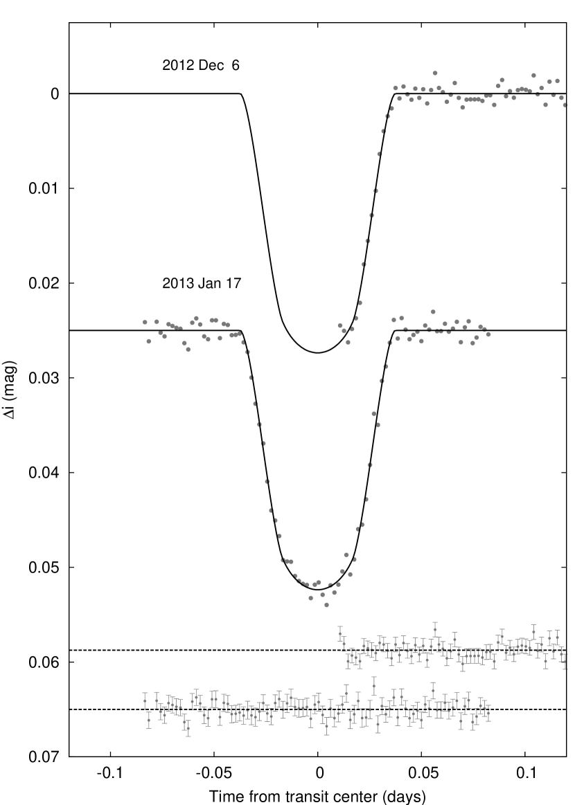
Figure 2.— Unbinned transit light curves for HAT-P-54, acquired with KeplerCam at the FLWO 1.2 m telescope. The light curves have been EPD- and TFA-processed, as described in Bakos et al. (2010). The dates of each event are indicated. Our best fit from the global modeling described in Section 3 is shown by the solid line. Residuals from the fit are displayed below in the same order as the original light curves. The error bars represent the photon and background shot noise, plus the readout noise.

Table 1 Differential photometry of HAT-P-54.

BJD	Mag	$\sigma_{\rm Mag}$	Mag(orig)	Filter	Instrument
(2,400,000$+$)
$55848.92474$	$0.03198$	$0.03424$	$\cdots$	$r$	HATNet
$55848.92799$	$0.02924$	$0.02342$	$\cdots$	$r$	HATNet
$55848.93068$	$-0.02762$	$0.03088$	$\cdots$	$r$	HATNet
$55848.93857$	$0.01040$	$0.02630$	$\cdots$	$r$	HATNet
$55848.94109$	$0.02453$	$0.02663$	$\cdots$	$r$	HATNet
$55848.94365$	$-0.02504$	$0.02325$	$\cdots$	$r$	HATNet
$55848.94856$	$0.03380$	$0.02507$	$\cdots$	$r$	HATNet
$55848.95633$	$0.03176$	$0.02936$	$\cdots$	$r$	HATNet
$55848.95889$	$-0.00495$	$0.02720$	$\cdots$	$r$	HATNet
$55848.96144$	$-0.02975$	$0.02380$	$\cdots$	$r$	HATNet

Note. — This table is available in a machine-readable form in the online journal. A portion is shown here for guidance regarding its form and content.

2.2. Spectroscopy

We carried out optical spectroscopic observations of HAT-P-54 using the Tillinghast Reflector Echelle Spectrograph (TRES; Fűresz, 2008) on the Tillinghast Reflector 1.5 m telescope at FLWO, and the HIRES spectrograph (Vogt et al., 1994) on the Keck-I 10 m telescope at MKO. A total of 14 TRES spectra were obtained using the medium resolution fiber on nights between 2012 Oct 28 and 2013 Nov 14, while 4 HIRES spectra, including an I₂-free template spectrum and 3 exposures with the I₂ cell, were obtained on the nights of 2013 Oct 18 and 19, and 2013 Dec 12.

The first two TRES observations were obtained at orbital phases of 0.74 and 0.25 (where phase 0 refers to the center of the transit) so as to efficiently rule out an eclipsing binary false positive. Subsequent observations were also clustered near these phases to maximize our sensitivity to a planet-induced orbital variation. We used exposure times ranging from 2400 s to 3000 s yielding a median S/N per resolution element (SNRe) of 26 near the Mg b region of the spectrum. The TRES observations were reduced to RVs and spectral line bisector spans (BSs) following Buchhave et al. (2010) and to measurements of the stellar atmospheric parameters ($T_{\rm eff\star}$, $\log{g}$, [Fe/H] and $v\sin{i}$) using the Stellar Parameter Classification (SPC) program (Buchhave et al., 2012). The RVs, obtained by conducting an order-by-order cross correlation against the strongest observed spectrum, show the predicted sense of variation in phase with the transit ephemeris, and with a semiamplitude of $132.6\pm 4.9$ $\rm m\,s^{-1}$ (Figure 3). The RMS scatter of the TRES residual RVs from our best-fit circular orbit model is 61 $\rm m\,s^{-1}$. Our model includes jitter in the amount of $53\pm 15$ $\rm m\,s^{-1}$ which is added in quadrature to the uncertainties output by the reduction pipeline. This jitter term is varied in the fit following Bieryla et al. (2014). The TRES RV residuals exhibit no evidence for a significant trend. Such a trend, if it were present, may indicate additional components (stellar or planetary) in the system.

The stellar atmospheric parameters derived from the TRES spectra, and listed in Table 3, indicate that the star is a cool ($T_{\rm eff\star}=4390\pm 50$ K), slowly rotating ($v\sin{i}=2.35\pm 0.50$ $\rm km\,s^{-1}$), low-metallicity ([Fe/H]$=-0.127\pm 0.080$), dwarf ($\log{g}=4.66\pm 0.10$, in cgs units). The errors listed are our estimates of the systematic uncertainties, based on observations of spectroscopic standard stars. Note that these uncertainties are general values adopted for the SPC program as applied to TRES, and do not include additional errors that may be present for cool stars. This issue is discussed further at the end of this subsection. For all four parameters, the scatter over the 14 observations is less than the estimated systematic uncertainty. Taken together, the RVs, light curves, and stellar parameters strongly indicate that this is a transiting planet system.

The HIRES observations were reduced to relative RV measurements in the barycentric frame following the procedure of Butler et al. (1996), and to BS measurements following Torres et al. (2007). The latter measurements were corrected for sky contamination following Hartman et al. (2011a). We note that the contamination was quite significant for the final HIRES observation, for which the resulting BS uncertainty is $>30$ $\rm m\,s^{-1}$(shown in Figure 3). When only 3 I₂-cell observations are available, the RV pipeline underestimates the errors, so we assumed an RV uncertainty of $5$ $\rm m\,s^{-1}$, which is typical for HIRES observations with a similar S/N. We note, however, that high stellar activity may induce RV jitter that is larger than this. As for TRES, we include a jitter term in the model which is varied in the fit. Our modeling yields a jitter for the HIRES observations of $3.2\pm 1.7$ $\rm m\,s^{-1}$. As a consistency check on our atmospheric parameters, we also applied SPC to the I₂-free template HIRES spectrum of HAT-P-54. The values, listed in Table 3, are remarkably similar to the mean parameters derived from the TRES spectra.

One note of caution regarding the atmospheric parameters is that the SPC results, which rely on synthetic spectra calculated from Kurucz model atmospheres (Castelli & Kurucz, 2003, 2004), are known to be unreliable for stars with $T_{\rm eff\star}<4700$ K. To mitigate this problem a prior on the gravity from the $Y^{2}$ isochrones (Yi et al., 2001) is adopted for cool stars which fixes the gravity to the range allowed by the stellar models for the initial temperature and metallicity guesses. For HAT-P-54, running the analysis without imposing a prior on the gravity yields $T_{\rm eff\star}=4330$ K and $\rm[Fe/H]=-0.12$, which is similar to the values found when the prior is used. While this, together with the similar results for the TRES and HIRES spectra, indicates that SPC is consistently finding the same parameters for the system, regardless of the spectroscopic instrument used or the manner in which the surface gravity is treated, due to the known systematic errors in the models we cannot claim with confidence that the parameters are accurate to within the stated uncertainties. A reanalysis using models that are more suitable for cool stars may yield parameter values that differ significantly from those presented here.

Figure 3.— Top panel: RV measurements from Keck-I/HIRES (filled circles) and FLWO 1.5 m/TRES (open triangles) for HAT-P-54 shown as a function of orbital phase, along with our best-fit circular model (solid line; see Table 4). Zero phase corresponds to the time of mid-transit. The center-of-mass velocity has been subtracted. Second panel: Velocity $O\!-\!C$ residuals from the best fit. The error bars include a “jitter” component ($3.2\pm 1.7$ $\rm m\,s^{-1}$, and $53\pm 15$ $\rm m\,s^{-1}$ for HIRES and TRES respectively) added in quadrature to the formal errors (see Section 2.2). The symbols are as in the upper panel. Third panel: Bisector spans (BS), with the mean value subtracted. For Keck/HIRES the measurement from the template spectrum is included. Note the different vertical scales of the panels.

Table 2 Relative radial velocities, bisector span measurements and stellar atmospheric parameters of HAT-P-54.

3. Analysis

3.1. Rejecting Blends

To rule out blend scenarios that could potentially explain the observations of HAT-P-54 we conducted an analysis similar to that done in Hartman et al. (2011c, 2012). We find that although model blended eclipsing binary systems can fit the available light curves, absolute photometry, and stellar atmospheric parameters, these models predict BS variations and RV variations that are inconsistent with the data (BS variations that are 200 $\rm m\,s^{-1}$ or greater, and RV variations of 1 $\rm km\,s^{-1}$ or greater). We conclude that HAT-P-54 is a transiting planet system, and not a blended stellar eclipsing binary system. We cannot, however, rule out the possibility that HAT-P-54 is a transiting planet orbiting one component of a binary star. High resolution imaging or continued RV monitoring is needed to check for stellar multiplicity (e.g. Adams et al., 2013). We caution that dilution from such a companion could alter the inferred planetary parameters. For the rest of this paper we assume that HAT-P-54 is an isolated star.

3.2. Determining Planetary and Stellar Parameters

We analyzed the system following Bakos et al. (2010) and Hartman et al. (2012). We adopted the stellar atmospheric parameters obtained by applying the SPC program (Buchhave et al., 2012) to the TRES spectra of HAT-P-54 (see Section 2.2). These values were used to determine fixed limb darkening coefficients taken from the Claret (2004) tabulations. We simultaneously modeled the RVs and light curves using an empirical noise model (EPD+TFA) to account for systematic variations in the Keplercam data. The modeling was done through a Differential Evolution Markov-Chain Monte Carlo procedure (ter Braak, 2006; Eastman et al., 2013) to explore the fitness landscape and determine the correlation between parameters. To speed up the process, we used standard linear algebra methods to optimize the parameters associated with our light curve noise model at each step in the Markov-Chain, rather than exploring their distribution as we do for the parameters used in the physical model. For the HIRES and TRES RV data we included a jitter term, added in quadrature to the formal errors, and varied in the fit as in Hartman et al. (2012), we also treated the zero-points of the two instruments as free and independent parameters in the fit. At each point in the resulting Markov-Chain we determined the stellar density from the fitted parameters, and used it, together with values for $T_{\rm eff\star}$ and $\rm[Fe/H]$ drawn from Normal distributions with mean and standard deviations set to the SPC values, to determine the mass, radius, age and luminosity of HAT-P-54 from theoretical stellar evolution models.

We carried out the analysis both fixing the eccentricity to zero and allowing it to vary. We used the Dartmouth (Dotter et al., 2008) stellar evolution models to determine the stellar parameters. In this respect we differ from prior HATNet discovery papers which used the Y² (Yi et al., 2001) isochrones, which are not optimal for low mass stars such as HAT-P-54. Figure 4 compares the measured effective temperature and stellar density for the fixed-circular, and free-eccentricity models to Dartmouth models. Because the star is a late K dwarf, its main sequence lifetime is greater than the age of the universe. Assuming the star must be less than 13.8 Gyr in age significantly restricts the range of density-temperature-metallicity combinations permitted by the stellar models. If the stellar evolution models are accurate, this effect puts a strong constraint on the eccentricity of the orbit (c.f. Hartman et al., 2011b).

When the eccentricity is fixed to zero, the combination of median density, best-fit metallicity, and best-fit temperature falls in a region of parameter space that is excluded by the Dartmouth models. In the $T_{\rm eff\star}$-$\rho_{\star}$ plane, with the metallicity fixed to the adopted value for the system, the observation falls at a density that is too high compared to the Dartmouth models. The observations are, however, within 1$\sigma$ of the permitted range. We also note that the minimum age included in the model is 1 Gyr, at which time the star is expected to be already slightly evolved (and thus lower density) than at the zero-age main sequence. When the eccentricity is allowed to vary the inferred stellar density is lower than in the fixed-circular case bringing the observations into good agreement with the Dartmouth models. We used the Weinberg et al. (2013) algorithm to estimate the Bayesian evidence for both the fixed circular and free-eccentricity models. In doing this we restrict the Markov Chains to consider only those links that are compatible with the stellar evolution models, and we include $T_{\rm eff\star}$ and $\rm[Fe/H]$ in calculating the fitness of each link. We find that, due to having fewer free parameters, the fixed-circular model is preferred over the free-eccentricity model (the evidence ratio is $\sim 60$). This does not mean that the orbit is circular, rather the number of high-precision RV observations is insufficient to place a strong constraint on the eccentricity. The 95% confidence upper-limit based on the free-eccentricity model is $e<0.074{}$, with the primary constraint being the requirement that the observations match to a stellar evolution model. If we do not require a match to the stellar evolution models, then the 95% confidence upper-limit on the eccentricity is $e<0.125$, with the constraint in this case coming only from the RVs.

For our final adopted parameters we use the fixed circular orbit model due to its higher Bayesian evidence. Additional high precision RV observations are necessary to robustly determine the eccentricity of this system. The chain of planetary and stellar parameters from our MCMC analysis is used to estimate the median parameter values together with their 68.3% (1$\sigma$) confidence intervals. These are listed in Tables 3 and 4. Note that because the values listed in the table are determined by calculating the parameter values at each link in the Markov-Chain and then taking their medians over the Chain, rather than adopting a self-consistent set of values associated with a particular model, slight numerical inconsistencies may be apparent when comparing different parameters in the table. Although this effect is well-known when presenting parameters based on a Bayesian analysis, we mention it here to ensure a proper interpretation of the values listed in the tables. Assuming a circular orbit, we conclude that the planet has a mass of $0.760\pm 0.032$ $M_{\rm J}$, and a radius of $0.944\pm 0.028$ $R_{\rm J}$, while the star has a mass of $0.645\pm 0.020$ $M_{\sun}$, and a radius of $0.617\pm 0.013$ $R_{\sun}$.

Figure 4.— Comparison between the measured values of $T_{\rm eff\star}$ and $\rho_{\star}$ (from SPC applied to the TRES spectra, and from our modeling of the light curves and RV data, respectively), and model isochrones taken from the Dartmouth series (Dotter et al., 2008). The best-fit values, and approximate 1$\sigma$ and 2$\sigma$ confidence ellipsoids are shown. In the left panel we show the measured values assuming a circular orbit in the fit, while in the right panel we show the values when the eccentricity is allowed to vary in the fit. The isochrones are shown for ages of 1.0 to 13.0 Gyr in 1 Gyr increments (this is the range over which the models are calculated). In both cases we fix the metallicity to $\rm[Fe/H]=-0.13$ for display purposes.

Table 3 Stellar Parameters for HAT-P-54

Parameter	Value	Source
Identifying Information
R.A. (h:m:s)	$06^{\mathrm{h}}39^{\mathrm{m}}35.53{\mathrm{s}}$	2MASS
Dec. (d:m:s)	$25{\arcdeg}28{\arcmin}57.1{\arcsec}$	2MASS
GSC ID	GSC 1884-00168	GSC
2MASS ID	2MASS 06393552+2528571	2MASS
EPID ID	202126849
Spectroscopic properties
$T_{\rm eff\star}$ (K)	$4390\pm 50$	TRES+SPC
$\rm[Fe/H]$	$-0.127\pm 0.080$	TRES+SPC
$v\sin{i}$ ($\rm km\,s^{-1}$)	$2.35\pm 0.50$	TRES+SPC
$\gamma_{\rm RV}$ ($\rm km\,s^{-1}$)	$30.84\pm 0.18$	TRES
Photometric properties
$B$ (mag)	$14.832\pm 0.070$	APASS
$V$ (mag)	$13.505\pm 0.060$	APASS
$g$ (mag)	$14.181\pm 0.020$	APASS
$r$ (mag)	$12.976\pm 0.020$	APASS
$i$ (mag)	$12.483\pm 0.020$	APASS
$J$ (mag)	$11.145\pm 0.025$	2MASS
$H$ (mag)	$10.487\pm 0.030$	2MASS
$K_{s}$ (mag)	$10.326\pm 0.019$	2MASS
$P_{\rm rot}$ (d)	$15.6$	HATNet
Derived properties
$M_{\star}$ ($M_{\sun}$)	$0.645\pm 0.020$	Isochrones+$\rho_{\star}$+SPC
$R_{\star}$ ($R_{\sun}$)	$0.617\pm 0.013$	Isochrones+$\rho_{\star}$+SPC
$\log{g_{\star}}$ (cgs)	$4.667\pm 0.012$	Isochrones+$\rho_{\star}$+SPC
$L_{\star}$ ($L_{\sun}$)	$0.1254\pm 0.0089$	Isochrones+$\rho_{\star}$+SPC
$M_{V}$ (mag)	$7.78\pm 0.13$	Isochrones+$\rho_{\star}$+SPC
$M_{K}$ (mag,ESO)	$4.720\pm 0.054$	Isochrones+$\rho_{\star}$+SPC
Age (Gyr)	$3.9_{-2.1}^{+4.3}$	Isochrones+$\rho_{\star}$+SPC
$A_{V}$ (mag)	$0.12\pm 0.11$	Isochrones+$\rho_{\star}$+SPC
Distance (pc)	$135.8\pm 3.5$	Isochrones+$\rho_{\star}$+SPC

Table 4Parameters for the transiting planet HAT-P-54b.

Parameter	Value
Light curve parameters
$P$ (days)	$3.799847\pm 0.000014{}$
$T_{c}$ (${\rm BJD}$)	$2456299.30370\pm 0.00024{}$
$T_{14}$ (days)	$0.07488\pm 0.00072{}$
$T_{12}=T_{34}$ (days)	$0.02055\pm 0.00093{}$
$a/R_{\star}$	$14.34\pm 0.22{}$
$\zeta/R_{\star}$	$35.36\pm 0.29{}$0
$R_{p}/R_{\star}$	$0.1572\pm 0.0020{}$
$b^{2}$	$0.550_{-0.015}^{+0.015}{}$
$b\equiv a\cos i/R_{\star}$	$0.741_{-0.011}^{+0.010}{}$
$i$ (deg)	$87.040\pm 0.084{}$0
Limb-darkening coefficients
$c_{1},i$ (linear term)	$0.4324{}$
$c_{2},i$ (quadratic term)	$0.2457{}$
$c_{1},r$	$0.5964{}$
$c_{2},r$	$0.1699{}$
RV parameters
$K$ ($\rm m\,s^{-1}$)	$132.6\pm 4.9{}$00
$e$	$<0.074{}$
RV jitter Keck-I/HIRES ($\rm m\,s^{-1}$)	$3.2\pm 1.7$
RV jitter FLWO 1.5 m/TRES ($\rm m\,s^{-1}$)	$53\pm 15$
Planetary parameters
$M_{p}$ ($M_{\rm J}$)	$0.760\pm 0.032{}$
$R_{p}$ ($R_{\rm J}$)	$0.944\pm 0.028{}$
$C(M_{p},R_{p})$	$0.30{}$
$\rho_{p}$ ($\rm g\,cm^{-3}$)	$1.118\pm 0.098{}$
$\log g_{p}$ (cgs)	$3.324\pm 0.027{}$
$a$ (AU)	$0.04117\pm 0.00043{}$
$T_{\rm eq}$ (K)	$818\pm 12{}$
$\Theta$	$0.1025\pm 0.0050{}$
$\langle F\rangle$ ($10^{8}$$\rm erg\,s^{-1}\,cm^{-2}$)	$1.010\pm 0.060{}$

3.3. Stellar Rotation

A search for continuous periodic variability in the residual HATNet light curve (i.e., residuals after subtracting our model transit light curve from the observations) using the Discrete Fourier Transform (DFT) reveals a signal at a frequency of $f=0.064247$ d^-1. This signal is suppressed in the TFA light curve, but detected with a S/N of 12.5 and an amplitude of $5.6$ mmag when only EPD is applied to the light curve. We tentatively identify this periodicity as the photometric rotation frequency of the star. The effective stellar rotation period in that case is $P=15.6$ d, which is close to four times the orbital period of the transiting planet. The EPD residual light curve phase-folded at this period, together with the DFT spectrum, and the Discrete Autocorrelation Function (DACF; Edelson & Krolik, 1988) of the light curve are shown in Figure 5. As seen in the DACF, the signal maintains coherence through at least six cycles. We note that the suppression by TFA of relatively low-frequency ($f<0.1$ d^-1) stellar variability due to rotation was previously seen in our analysis of HAT-P-11 (Bakos et al., 2010), where a $P\sim 30$ d signal was found in the EPD HATNet light curve, but not found in the TFA light curve. Subsequent Kepler observations confirmed the variability seen in the HATNet EPD data.

As a consistency check we may also estimate an upper limit on the equatorial rotation period (assuming $\sin i=1$) using the spectroscopically determined $v\sin{i}$ together with $R_{\star}$ as determined in Section 3.2. We find $P<13.1^{+3.6}_{-2.4}$ d which is consistent with the photometric rotation period to within $1\sigma$.

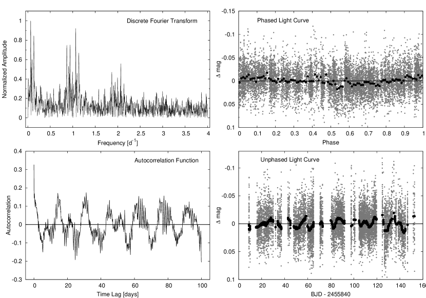
Figure 5.— Detection of quasi-periodic photometric variability in the HATNet light curve of HAT-P-54, which we attribute to spots on the surface of the rotating star. Upper left: the Discrete Fourier Transform of the EPD-filtered HATNet light curve of HAT-P-54. The amplitude has been normalized to that of the highest peak, seen at a frequency of $f=0.06397$ d^-1 ($P=15.6$ d), and with an $S/N$ of 12.5. We identify this as the photometric rotation frequency of the star. Lower left: the Discrete Autocorrelation Function of the same light curve, calculated following Edelson & Krolik (1988), and using a step of 0.05 d. The first significant peak seen at a lag of $15.6$ d, corresponds to the rotation period. The peak repeats with comparable amplitude through six cycles, indicating a long coherence time for the signal. Upper right: the differential HATNet light curve phase-folded at the photometric rotation period of the star. The light grey points show the individual measurements, the dark filled circles show the light curve binned in phase using a bin size of 0.01. The solid line shows $\Delta m=0$ for reference. Lower right: un-phased light curve plotted as a function of time. In this case the dark filled circles show the median light curve (calculated using a moving window of $1.0$ d). Variations with a peak to peak amplitude of $\sim 0.01$ mag are apparent.

4. Discussion

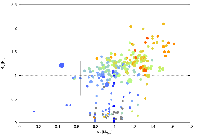
Figure 6.— Planetary radius versus stellar mass for transiting extrasolar planets (and brown dwarfs) with well measured masses (from radial velocities or transit timing variations). Size of the points scales with the cube-root of the mass. In the color version of this figure, color indicates equilibrium temperature of the planet (Bond albedo fixed at 0, full redistribution of flux assumed) on a rough scale of red being $T_{\rm eq}>2000$ K, green $\approx 1500$ K and blue $\approx 1000$ K. Small blue triangles show the major Solar System planets. HAT-P-54b is marked with a large cross.

In this paper we have presented the discovery and characterization of HAT-P-54b, a compact hot Jupiter orbiting a late K dwarf star. With a mass of between that of Saturn and Jupiter ($0.760\pm 0.032$ $M_{\rm J}$), and radius of $0.944\pm 0.028$ $R_{\rm J}$, HAT-P-54b is compact; smaller in radius than $\sim 92$% of the known transiting planets with measured masses greater than that of Saturn. HAT-P-54b also orbits one of the lowest mass stars ($M_{\star}$= $0.64$ $M_{\sun}$) known to have a close-in gas-giant planet, and it is the lowest mass planet host discovered by the HATNet survey. Only 3 stars with smaller mass are known to host a planet with $0.1<M_{p}<13$ $M_{\rm J}$, and $P<$30 d. These are WASP-43 (Hellier et al., 2011), WASP-80 (Triaud et al., 2013), and Kepler-45 (Johnson et al., 2012). A planet or brown dwarf with $M_{p}=18.4$ $M_{\rm J}$ has also been discovered on a 1.3 d period orbit around the M dwarf HD 41004 B (Zucker et al., 2004). Thus, the HAT-P-54 system has several atypical properties which make it an interesting object for further study. These findings are well demonstrated by Fig. 6, displaying the planetary radius versus the stellar mass. HAT-P-54 is shown by a cross at the left (small stellar mass) and low (small planetary radius) side of the hot Jupiter population. Among a few other things worth noting in Fig. 6 is the correlation of planet radius with stellar mass, which is a manifestation of the previously found planet radius vs. stellar flux dependence (see Spiegel & Burrows, 2013, and references therein). Also visible is the paucity of “sub-Jovian” planets with radii $0.4\,R_{\rm J}\lesssim R_{p}\lesssim 0.7\,R_{\rm J}$, as previously noted by Beaugé & Nesvorný (2013) using the period–planetary radius plane. Finally, the emerging population of highly inflated Jupiters (Hartman et al., 2012) also appears detached from the rest of the planets on the top right side of the figure.

Of particular interest is the fact that HAT-P-54 lies within field 0 of the K2 mission. Observations of this field began on 2014 Mar 8, and are expected to finish on 2014 May 30. A proposal to observe this star in long cadence mode, together with other candidate transiting planet hosts identified by HATNet, has been accepted through the Kepler Guest Observing program. As far as we are aware, HAT-P-54 is the only currently known transiting planet within this field. Several other transiting planets are known near the K2 field, however none of them are among the list of targets selected for observations with K2, and all are outside the field defined by the selected targets. The RV-detected planet HD 50554b (Fischer et al., 2002), which is not known to be transiting, is also in field 0 of the K2 mission. Very high precision Kepler observations of HAT-P-54 will provide a wealth of information that will be used to precisely measure the system parameters, and possibly detect subtle features, such as spot crossings by the transiting planet, and reflected light, among others.

Acknowledgements

HATNet operations have been funded by NASA grants NNG04GN74G and NNX13AJ15G. Follow-up of HATNet targets has been partially supported through NSF grant AST-1108686. G.Á.B., Z.C. and K.P. acknowledge partial support from NASA grant NNX09AB29G. K.P. acknowledges support from NASA grant NNX13AQ62G. G.T. acknowledges partial support from NASA grant NNX14AB83G. We acknowledge partial support also from the Kepler Mission under NASA Cooperative Agreement NCC2-1390 (D.W.L., PI). G.K. thanks the Hungarian Scientific Research Foundation (OTKA) for support through grant K-81373. Based in part on observations obtained at the W. M. Keck Observatory, which is operated by the University of California and the California Institute of Technology. Keck time has been granted by NASA (N133Hr). Data presented in this paper are based on observations obtained at the HAT station at the Submillimeter Array of SAO, and the HAT station at the Fred Lawrence Whipple Observatory of SAO. Data are also based on observations with the Fred Lawrence Whipple Observatory 1.5 m and 1.2 m telescopes of SAO. The authors wish to recognize and acknowledge the very significant cultural role and reverence that the summit of Mauna Kea has always had within the indigenous Hawaiian community. We are most fortunate to have the opportunity to conduct observations from this mountain.

References

- Adams et al. (2013) Adams, E. R., Dupree, A. K., Kulesa, C., & McCarthy, D. 2013, AJ, 146, 9
- Bakos et al. (2004) Bakos, G., Noyes, R. W., Kovács, G., et al. 2004, PASP, 116, 266
- Bakos et al. (2010) Bakos, G. Á., Torres, G., Pál, A., et al. 2010, ApJ, 710, 1724
- Barclay et al. (2012) Barclay, T., Huber, D., Rowe, J. F., et al. 2012, ApJ, 761, 53
- Beaugé & Nesvorný (2013) Beaugé, C., & Nesvorný, D. 2013, ApJ, 763, 12
- Béky et al. (2014) Béky, B., Holman, M. J., Kipping, D. M., & Noyes, R. W. 2014, ArXiv e-prints, 1403.7526
- Bieryla et al. (2014) Bieryla, A., Hartman, J. D., Bakos, G. Á., et al. 2014, AJ, 147, 84
- Borucki et al. (2009) Borucki, W. J., Koch, D., Jenkins, J., et al. 2009, Science, 325, 709
- Buchhave et al. (2010) Buchhave, L. A., Bakos, G. Á., Hartman, J. D., et al. 2010, ApJ, 720, 1118
- Buchhave et al. (2012) Buchhave, L. A., Latham, D. W., Johansen, A., et al. 2012, Nature, 486, 375
- Butler et al. (1996) Butler, R. P., Marcy, G. W., Williams, E., et al. 1996, PASP, 108, 500
- Cardelli et al. (1989) Cardelli, J. A., Clayton, G. C., & Mathis, J. S. 1989, ApJ, 345, 245
- Castelli & Kurucz (2003) Castelli, F., & Kurucz, R. L. 2003, in IAU Symposium, Vol. 210, Modelling of Stellar Atmospheres, ed. N. Piskunov, W. W. Weiss, & D. F. Gray, 20P
- Castelli & Kurucz (2004) Castelli, F., & Kurucz, R. L. 2004, ArXiv Astrophysics e-prints
- Claret (2004) Claret, A. 2004, A&A, 428, 1001
- Deming et al. (2011) Deming, D., Sada, P. V., Jackson, B., et al. 2011, ApJ, 740, 33
- Dotter et al. (2008) Dotter, A., Chaboyer, B., Jevremović, D., et al. 2008, ApJS, 178, 89
- Eastman et al. (2013) Eastman, J., Gaudi, B. S., & Agol, E. 2013, PASP, 125, 83
- Edelson & Krolik (1988) Edelson, R. A., & Krolik, J. H. 1988, ApJ, 333, 646
- Fűresz (2008) Fűresz, G. 2008, PhD thesis, Univ. of Szeged, Hungary
- Fischer et al. (2002) Fischer, D. A., Marcy, G. W., Butler, R. P., et al. 2002, PASP, 114, 529
- Hansen & Barman (2007) Hansen, B. M. S., & Barman, T. 2007, ApJ, 671, 861
- Hartman et al. (2011a) Hartman, J. D., Bakos, G. Á., Sato, B., et al. 2011a, ApJ, 726, 52
- Hartman et al. (2011b) Hartman, J. D., Bakos, G. Á., Kipping, D. M., et al. 2011b, ApJ, 728, 138
- Hartman et al. (2011c) Hartman, J. D., Bakos, G. Á., Torres, G., et al. 2011c, ApJ, 742, 59
- Hartman et al. (2012) Hartman, J. D., Bakos, G. Á., Béky, B., et al. 2012, AJ, 144, 139
- Hellier et al. (2011) Hellier, C., Anderson, D. R., Collier Cameron, A., et al. 2011, A&A, 535, L7
- Howell et al. (2014) Howell, S. B., Sobeck, C., Haas, M., et al. 2014, ArXiv e-prints, 1402.5163
- Jackson et al. (2012) Jackson, B. K., Lewis, N. K., Barnes, J. W., et al. 2012, ApJ, 751, 112
- Johnson et al. (2012) Johnson, J. A., Gazak, J. Z., Apps, K., et al. 2012, AJ, 143, 111
- Kipping & Bakos (2011) Kipping, D., & Bakos, G. 2011, ApJ, 733, 36
- Kovács et al. (2005) Kovács, G., Bakos, G., & Noyes, R. W. 2005, MNRAS, 356, 557
- Kovács et al. (2002) Kovács, G., Zucker, S., & Mazeh, T. 2002, A&A, 391, 369
- Morris et al. (2013) Morris, B. M., Mandell, A. M., & Deming, D. 2013, ApJ, 764, L22
- O’Donovan et al. (2006) O’Donovan, F. T., Charbonneau, D., Mandushev, G., et al. 2006, ApJ, 651, L61
- Pál et al. (2008) Pál, A., Bakos, G. Á., Torres, G., et al. 2008, ApJ, 680, 1450
- Sanchis-Ojeda & Winn (2011) Sanchis-Ojeda, R., & Winn, J. N. 2011, ApJ, 743, 61
- Spiegel & Burrows (2013) Spiegel, D. S., & Burrows, A. 2013, ApJ, 772, 76
- ter Braak (2006) ter Braak, C. J. F. 2006, Statistics and Computing, 16, 239
- Torres et al. (2007) Torres, G., Bakos, G. Á., Kovács, G., et al. 2007, ApJ, 666, L121
- Triaud et al. (2013) Triaud, A. H. M. J., Anderson, D. R., Collier Cameron, A., et al. 2013, A&A, 551, A80
- Vogt et al. (1994) Vogt, S. S., Allen, S. L., Bigelow, B. C., et al. 1994, in Society of Photo-Optical Instrumentation Engineers (SPIE) Conference Series, Vol. 2198, Society of Photo-Optical Instrumentation Engineers (SPIE) Conference Series, ed. D. L. Crawford & E. R. Craine, 362
- Weinberg et al. (2013) Weinberg, M. D., Yoon, I., & Katz, N. 2013, ArXiv e-prints, 1301.3156
- Welsh et al. (2010) Welsh, W. F., Orosz, J. A., Seager, S., et al. 2010, ApJ, 713, L145
- Yi et al. (2001) Yi, S., Demarque, P., Kim, Y.-C., et al. 2001, ApJS, 136, 417
- Zucker et al. (2004) Zucker, S., Mazeh, T., Santos, N. C., Udry, S., & Mayor, M. 2004, A&A, 426, 695