Subdiffraction-limited imaging based on longitudinal modes in a spatially dispersive slab
Abstract
It was proposed that a flat silver layer could be used to form a sub-diffraction limited image when illuminated near its surface plasmon resonance frequency [J. B. Pendry, Phys. Rev. Lett. 86, 3966 (2000)]. In this paper, we study the possibility of obtaining sub diffraction resolution using a different mechanism, with no surface plasmons involved. Instead, by taking into account the non-local response of a thin silver slab, we show that longitudinal modes contribute to the formation of a sub-diffraction limited image in a frequency regime above the plasma frequency. The differences between these two distinct mechanisms are studied and explained.
I introduction
In 2000, it was suggested that a thin planar metallic slab can perform as a lens capable of producing an image with sub-diffraction limited (SDL) resolution pendry . In this seminal paper, Pendry showed that by using a thin metallic slab, only few tens of nanometers thick, which is excited with light near its surface plasmon (SP) resonance frequency, an image with SDL size can be obtained, due to the high momentum frequency components of the SP modes that are supported by the interfaces between the metallic slab and the dielectric medium surrounding it. This concept of a homogeneous slab performing as a lens was a variant (perhaps more realistic) based on previous work of Veselago that showed that ideal negative index slab, behaves as a lens veselago . Pendry also claimed that the resolution of such an ideal negative index slab is not limited pendry . It is now common to coin the ideal negative index slab configuration as a “perfect lens”, while a thin metallic layer is now defined as a “poor man’s lens”. Both types of lenses became the subject of debate and controversy collin . The discussion was further stimulated by the experimental demonstration of the “poor man’s lens”, obtaining resolution of the order of ( being the vacuum wavelength) N_Fang ; blaikie ; Fang2 . Part of the debate regarding the poor man’s lens was concerned with the fact that a momentum cutoff of the SP modes is inherent, due to the nonlocal response of the metal permittivity function stockman ; ramakrishna ; ruppin-lens ; ruppin_kempa . In the nonlocal description, the permittivity function is described by , i.e. it is a function of both the optical frequency and the propagation constant , due to temporal and spatial dispersion, respectively. For small -vectors, one can neglect spatial dispersion and assume that . However, for large -vectors, the SP modes reach a momentum cutoff resulting in a fundamental resolution limit for perfect imaging. A detailed analysis, however, showed that the “poor man’s lens” performance is very similar under both local and nonlocal approximations, because the ohmic losses inherent to the metal deteriorate the image even more drastically as compared with nonlocal effects david_sci_rep . Nonlocal effects for metallic slabs are pronounced when the slab thickness is less than the 10-nm regime. For these dimensions, it was shown that the absorption spectrum above the plasma frequency exhibits oscillations due to Fabry-Perot (FP) resonances of longitudinal modes which are modes with zero magnetic field, and electric field vector parallel to the propagation vector . Longitudinal modes satisfy the macroscopic Maxwell’s equations when agranovich_ginzburg ; silin ; forstmann-book . For several metals such as alkali metals and silver, a phenomenological description of can be obtained by employing the linearized hydrodynamic model feibelman ; pitarke ; boardman-ruppin ; boardman-book ; hanson ; mortensen . This model successfully reproduces the appearance of longitudinal mode resonances which were experimentally observed for thin layered metals Anderegg and offers a qualitative explanation for the blue shifting of the localized SP resonance observed in silver nanoparticles ciraci ; raza2 ; pasha ; toscano . These results cannot be explained with local models. However, the validity of this model is challenged to account for quantum sized effects teperik-quantum-corrected ; stella-hydro-quantum ; esteban-quantum-corrected ; monreal . In general, a full quantum-mechanical calculation is needed for an accurate account of the non-local response. However, the longitudinal mode resonance effect (described below) that is in the heart of this paper, is fully accounted for by the hydrodynamic model. In this paper, we propose a different physical concept for achieving SDL imaging, taking advantage of the longitudinal modes within a thin metallic slab that is described by the hydrodynamic model. The SDL imaging occurs for discrete frequencies satisfying . This frequency regime is different from the original proposal of the “poor man’s lens”, in which the incident illumination frequency is in the vicinity of the SP resonance frequency . Furthermore, the underlying physical mechanism of the two approaches is different. In the original proposal, the high- components of the source are reconstructed in the image by the SP resonance surface modes which support high spatial frequency components. In contrast, our approach is not based on surface modes. Instead, the high- components are transferred to the image plane by the longitudinal modes, which typically have propagation constants more than an order of magnitude larger than the vacuum propagation constant . The paper is structured as follows. In Sec. II we describe the modes inherent to the nonlocal slab-lens geometry. In Sec. III we present results based on this formalism. Sec. IV concludes the paper.
II Modal analysis
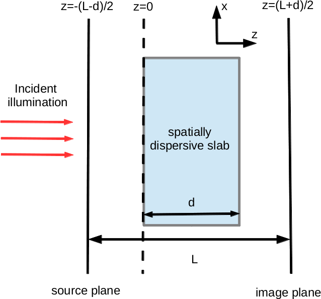
Our lens geometry consists of a slab infinitely extending along the and coordinates and bound between and (see schematic in Fig. 1). The image and source planes are located at and respectively. In our analysis we assume that the slab is surrounded by vacuum. We consider TM polarization illumination, i.e. , for which plasmonic and longitudinal modes exist. The permittivity of the slab is described by the hydrodynamic model. From this model it follows that for transverse modes () the permittivity function follows the well-known Drude model , while for the longitudinal modes () the material response is given by . Here, is the damping constant, and defines the strength of the nonlocal response. The electric fields of the transverse modes are given by , and the propagation constant of the transverse mode satisfies the dispersion relation . The electric fields of the longitudinal mode is given by , and its propagation constant is given by , which follows directly from the longitudinal mode dispersion relation . Because the spatially dispersive slab supports twice the number of modes a non-spatially dispersive slab does, an additional boundary condition (ABC) is needed other than the two conventional conditions of continuity of the transverse fields, in order to solve for all modal amplitudes agranovich_ginzburg ; forstmann-book ; Silveirinha ; moreau . For an air/metal interface the set of boundary conditions we assume are the continuity of , and the normal current . Employing these boundary conditions and preserving the continuity of , one obtains the expression for the complex transmission amplitude melnyk . For completeness, the derivation for the transmission amplitude is presented in the Appendix.
III Results and interpretation
We now turn into studying the transmission through an Ag slab for the following parameters blaber : eV, , and . Here and c are the Fermi velocity and the speed of light in vacuum respectively. Possible surface roughness of the layer is not taken into account in our simplified model (see Ref. feibelman Sec. 4D). We continue our study assuming this set of parameters, although the concepts derived below are general and support any spatially dispersive material which can be described by the hydrodynamic model. In Fig. 2(a) we plot as a function of and for the case of SP resonance, where the frequency is in the vicinity of , assuming layer thickness of nm. Two SP resonances with components below the light line are observed. From previous studies khurgin ; pendry2 ; collin ; orenstein , it is known that it is the interplay between the two modes that allows for the reconstruction of an image with SDL resolution, due to the very high transmission coefficients of plane waves with large (mind the logarithmic scale bar).
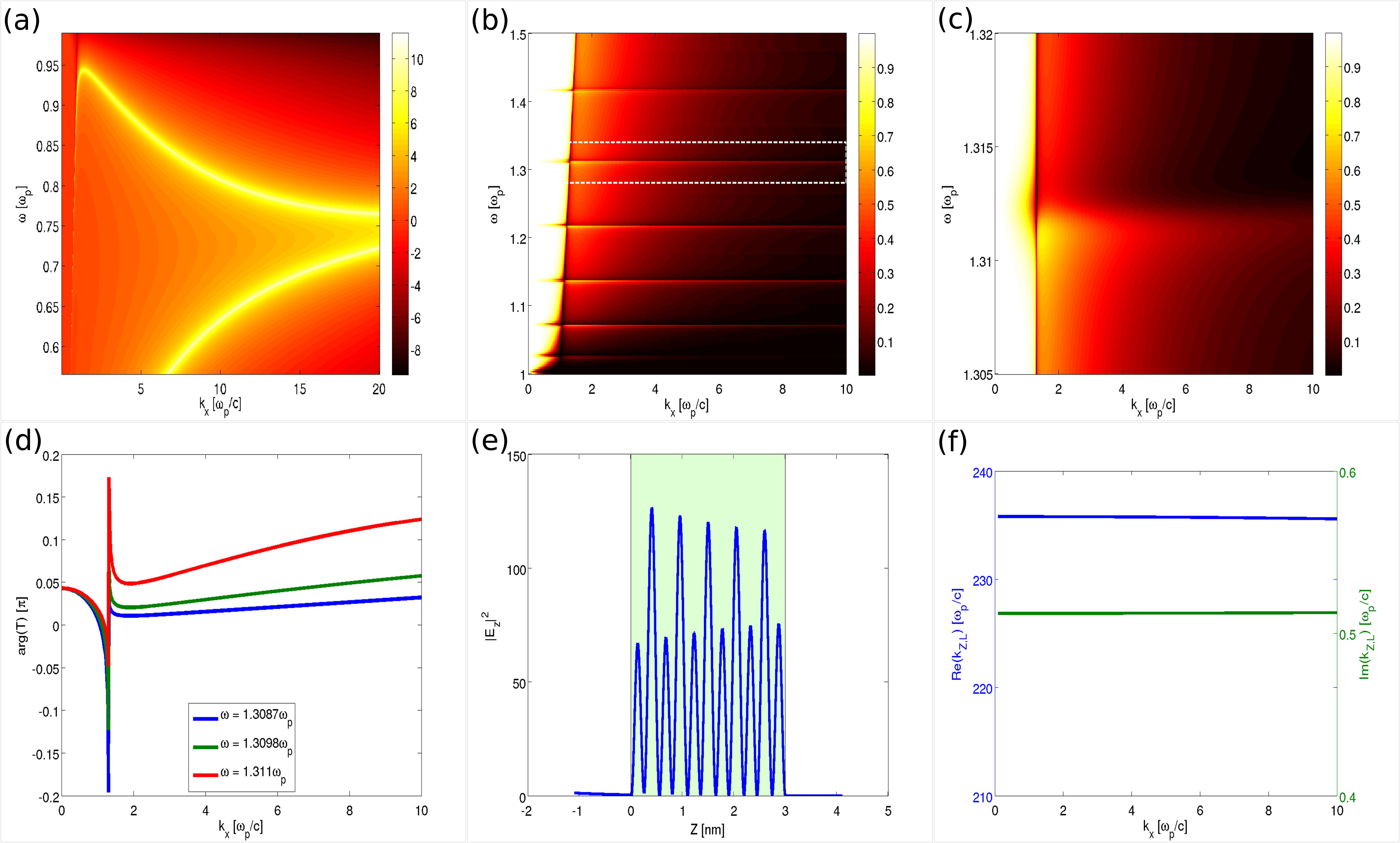
In Fig. 2(b) we calculate assuming the same slab thickness, however we now consider a different frequency interval ). In this frequency range, becomes predominantly real. Moreover, for the assumed ultrathin slab dimensions, the longitudinal modes exhibit distinguishable FP resonances at discrete frequencies satisfying , where is an odd number (Ref. (forstmann-book, , section 3.2)). A detailed view of one of these FP modes () at , is shown in Fig. 2(c). At these resonance frequencies, the spectrum of shows transmission peaks, which are nearly uniform in frequency over a large range of values. Therefore, the transmission spectrum at one of these resonant frequencies seems to be more appealing for reconstruction of an SDL image (which typically contains a large span of values) as compared to the SP resonance case, which is more dispersive in nature, as shown in Fig. 2(a). On the other hand, the overall transmission magnitude of these longitudinal modes is lower as compared to the SP modes (note that Fig. 2(a) is in logarithmic scale while Fig. 2(b) is not!). In addition to the FP transmission peaks which are evident for large values of , we also notice in Fig. 2(b) the existence of a region with nearly uniform transmission for low values of which are above the light cone. In this region the transmission is , besides discrete dips in transmission corresponding to the FP modes. The FP modes exist mathematically for , but since grows with , the resonance effect diminishes with the frequency. We next turn into a further comparison between the two approaches, with the goal of identifying the inherent properties and advantages of each approach.
To perfectly image a line source, one needs both the transmission magnitude and the transmission phase to be constant with (Ref. chew Sec. 2.2.1). In Fig. 2(d) we plot the normalized phase of transmission as a function of for several frequencies near , to estimate how uniform is the phase for different spatial frequencies. In Fig.2(e) we plot the magnitude of the in the slab for a specific FP resonance of the longitudinal modes ( and ). In Fig. 2(f) we plot the dependence of the real and imaginary part of , as a function of , for . It is seen that the variation in is negligible (% in its real value and% in its imaginary value). This is primarily due to its large value, which is the key reason for the FP transmission resonances shown in Fig. 2(b) being nearly flat with .
To estimate the imaging capabilities of the lens, we define two point spread functions (PSF), by calculating the transmission function at the image plane obtained by summation of an infinite number of plane waves according to:
| (1) |
| (2) |
Here and correspond to the PSF of the and electric field components respectively. The vacuum propagation constant is defined by Equations (1) and (2) are defined for the case of polarized illumination. Following these definitions, we also define the total PSF in the image plane as:
| (3) |
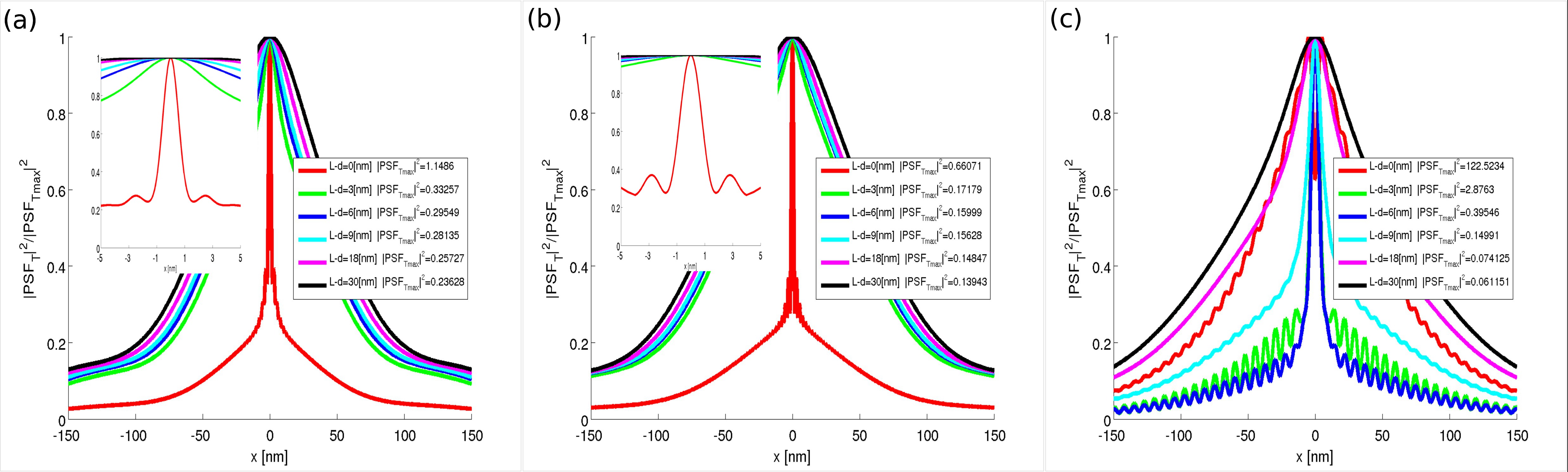
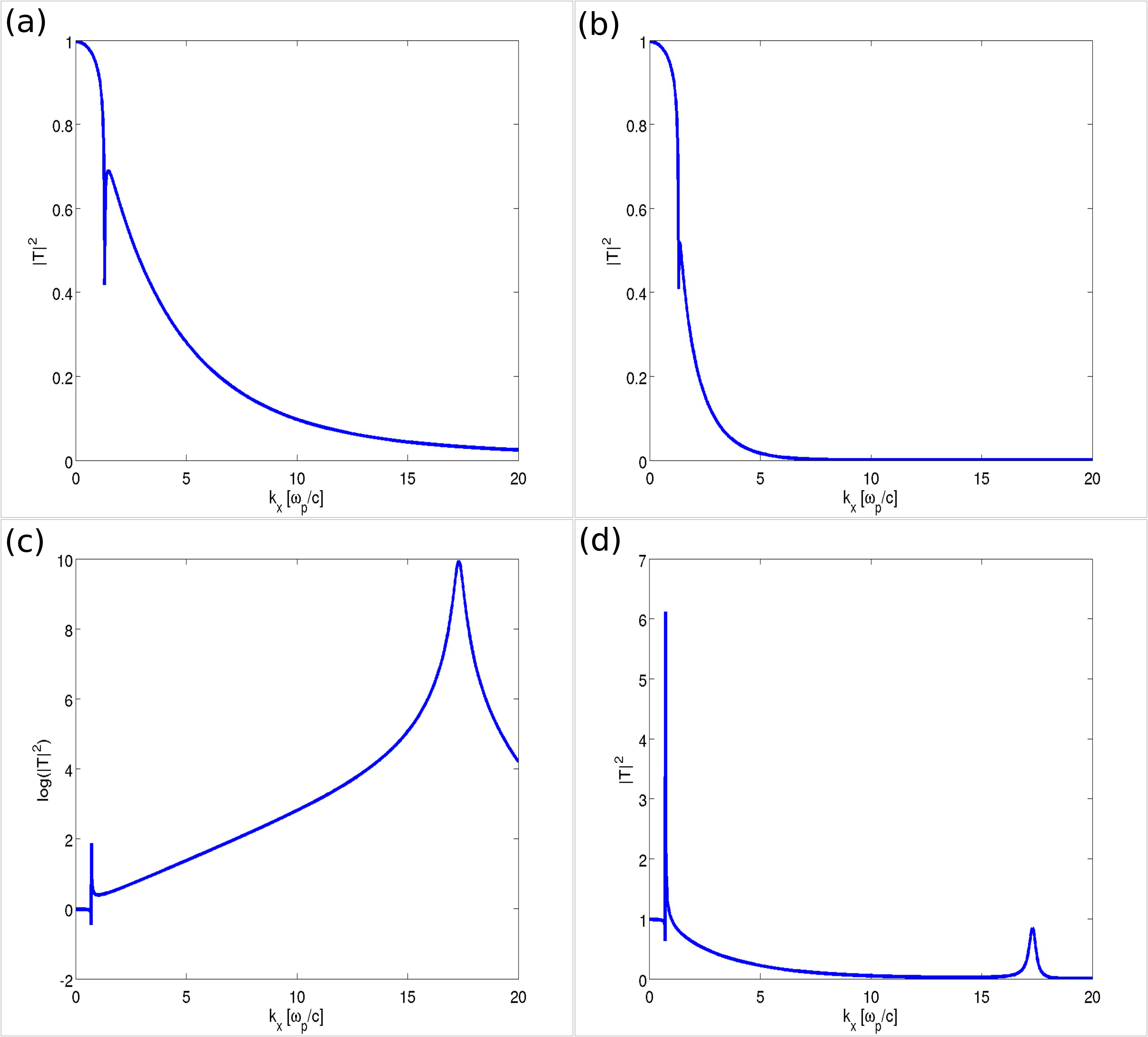
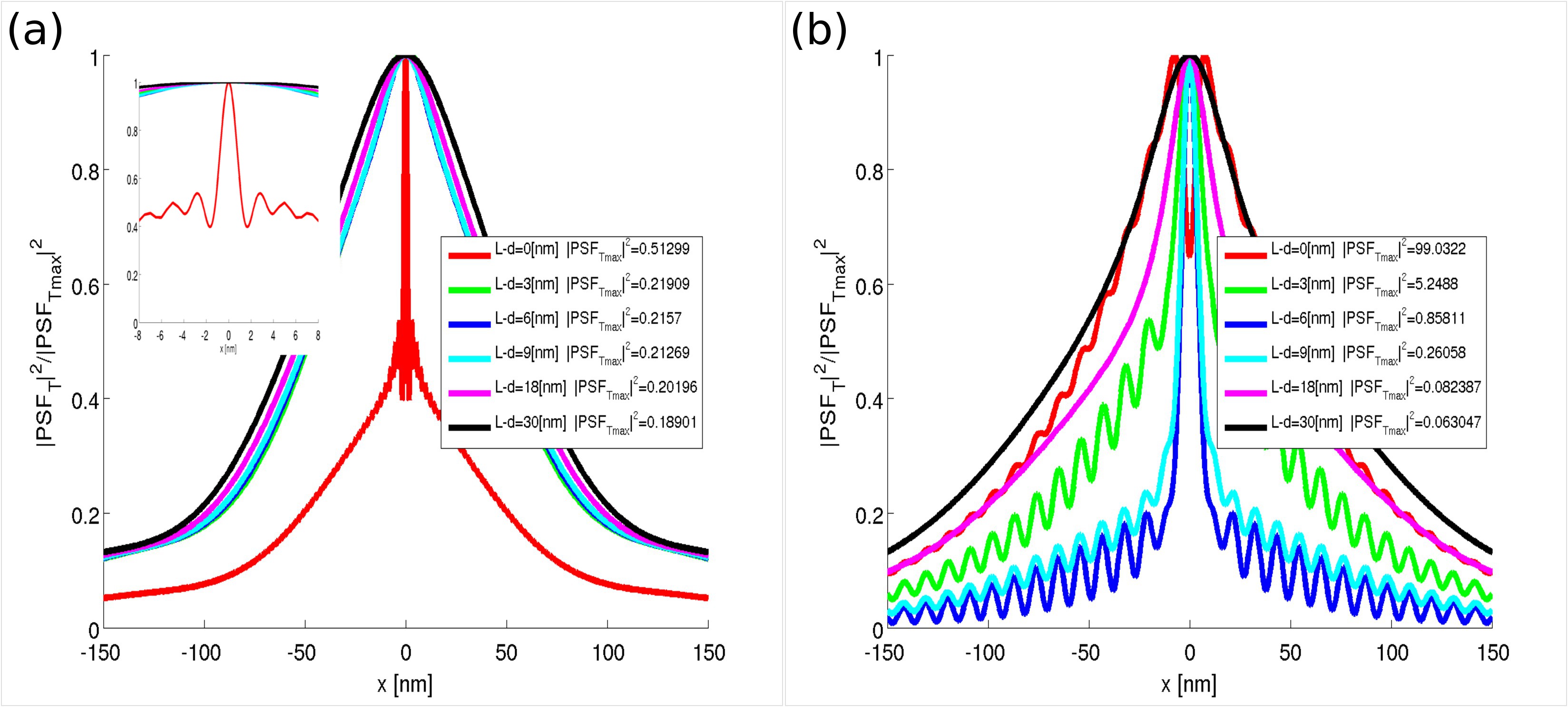
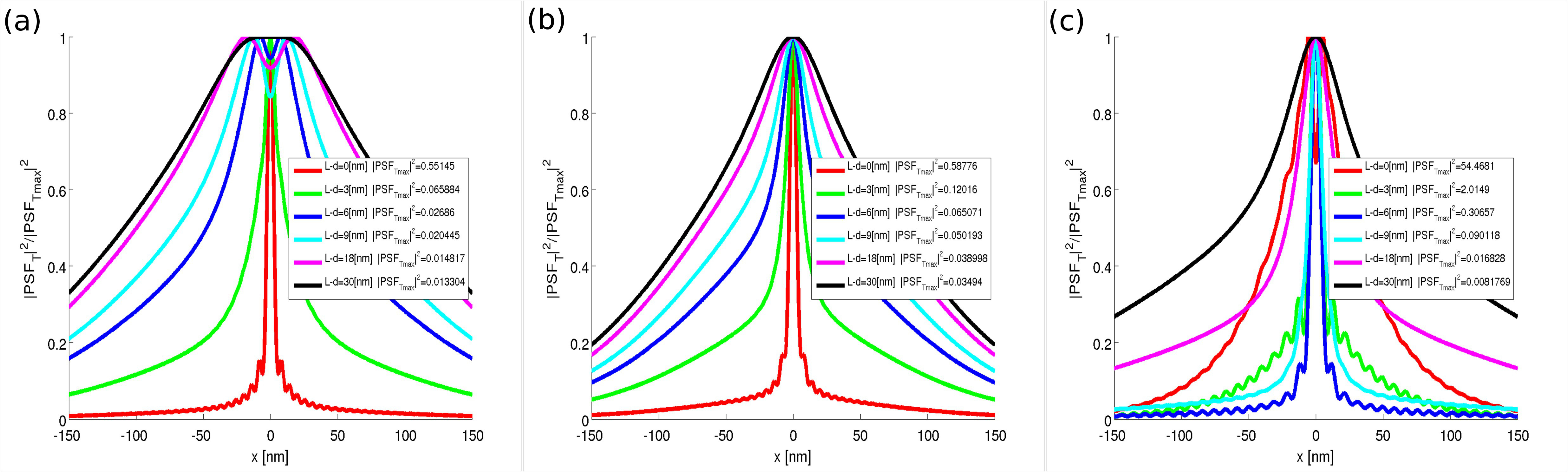
In Fig. 3 the normalized transmission magnitude in the image plane is plotted for several imaging distances . The legend shows the normalization factor for each imaging distance. Fig. 3(a,b) show the results obtained for the longitudinal mode FP resonance with () and (), respectively. Fig. 3(c) is calculated for , corresponding to the plasmonic resonance. For the case where the source is positioned at the surface of the slab (, red line) the longitudinal mode FP mechanism results in an ultra-narrow FWHM of less than 2 nm, for both FP resonances. However, when the imaging distance increases, the FWHM increases and substantial broadening of the is observed. We note that the PSFs of the two FP resonances (Figs. 3(a,b)) are relatively similar. Once again, this is the outcome of the relatively flat dispersion curves of the FP modes. In contrast, the plasmonic resonance (Fig. 3(c)) behaves very differently. One may observe that the is narrower when the source is slightly away of the surface, ( and nm, green and blue lines, respectively which have PSF FWHM of 6 nm) compared with the case where the source is located on the surface (). The question arises, why for the plasmonic resonance case, the PSF narrows with increasing imaging distance, while for the longitudinal mode case, the PSF always broadens with the increase in imaging distance. The underlying reason is revealed from the transmission spectrum, calculated for several imaging distances. In Fig. 4(a,b), we plot the transmission magnitude as a function of of the FP resonance at for and nm. It is seen that for components larger than the vacuum light line (i.e. ) we obtain a rapid decay of the transmission for a distance of nm, compared with the case. This observation explains the broader PSF for the latter case (Fig. 3(a), blue vs. red curve).
The transmission spectrum is also useful for explaining the PSF results of the plasmonic resonance. In Fig. 4(c,d), it is seen that for nm the transmission spectrum is more flat as compared with the case (mind that Fig. 4(c) is in logarithmic scale). Therefore, the PSF becomes narrower (see Fig. 3(c), blue vs. red line).
The relatively large imaginary component of , sets a practical limitation on the slab thickness, preventing the use of slabs thicker than nm. Indeed, this thickness is known to be the critical dimension for observing non-local effects in Ag yanai . By increasing beyond nm, the PSF becomes wider, and the transmission magnitude reduces. This is shown in Fig. 5 presenting the calculated for nm and two frequencies, (corresponding to the FP resonance with ) and . The FWHM of is now nm for the longitudinal FP resonance case with , which is about times larger than the FWHM obtained for nm. For the plasmonic resonance case, the increase of the layer thickness has a more moderate effect. For the case shown in Fig. 3(c), with nm, the FWHM is nm, while for the case shown in Fig. 5(b) with nm, the FWHM is found increase only slightly, to nm.
Finally, we consider the possibility of using a slab made of potassium (K) rather than Ag. We assume the following parameters for K blaber : eV, , and . Because the plasma frequency of K is lower than that of Ag and is in the soft UV range, this metal might be more appealing for practical demonstrations of the SDL imaging effect in the UV, e.g. for lithography applications. In Fig. 6(a,b) we show the PSF for the () and () FP resonances, calculated for a K layer thickness of nm. In Fig. 6(c) we show the PSF for the plasmonic resonance case (). Because of the higher ohmic losses of this metal, the PSF in all three cases is evidently wider as compared to the Ag case. Yet, it may still be a more practical choice from the technological point of view Anderegg .
IV Conclusion
In conclusion, we have analyzed the scenario of SDL imaging based on longitudinal modes excited in a spatially dispersive metallic slab above the metal plasma frequency. Our results show that in this regime, for frequencies satisfying ( is an odd number) a transmission spectrum nearly flat with is obtained, resulting in an ultra narrow PSF for the case of full contact (). This PSF is significantly more narrow than the one obtained with the conventional plasmonic based “poor man’s lens” operated near . However, when is larger than few nanometers, the situation is inverted and the plasmonic “poor men lens” becomes a much better choice as it provides much narrower PSF. Another interesting difference is related to the wavelength of choice. With our proposed approach, the frequency of operation can be tuned (either by changing the layer thickness, or by choosing a higher order FP resonance), while for the SP resonance case the operation frequency is fixed in the vicinity of . We believe that the proposed concept could have several useful applications for fields such as nano-lithography, sensing, and microscopy, to name a few.
Appendix A Calculation of the transmission amplitude for a spatially dispersive slab
For completeness, we derive here the expression for the transmission amplitude for the case of a spatially dispersive slab surrounded by local media. Similar derivations are available for the slab case melnyk ; forstmann-book ; david_sci_rep , and the more general periodic case yanai . The slab geometry and the field amplitudes are depicted in Fig. 7. The incident and reflected amplitudes are denoted by and respectively. In the slab, we define two transverse mode amplitudes and , propagating and counter-propagating respectively, and two longitudinal mode amplitudes and . The transmitted mode amplitude is . To derive the complex transmission amplitude , we match all fields according to the assumed ABC. For this geometry, there are three types of incidence of the various modes:
-
1.
Transverse mode incident from a spatially non-dispersive medium onto a spatially dispersive medium
-
2.
Transverse mode incident from a spatially dispersive medium onto a spatially non-dispersive medium
-
3.
Longitudinal mode incident from a spatially dispersive medium onto a spatially non-dispersive medium
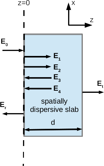
Figure 7: Schematic showing the field components of the various modes for the scenario of a spatially dispersive slab surrounded by local media.
Employing the ABC, the transmission and reflection coefficients for these three incidence types can be derived:
| (4a) |
| (4b) |
| (4c) |
| (4d) |
| (4e) |
| (4f) |
| (4g) |
| (4h) |
| (4i) |
For these nine coefficients, and are for reflection and transmission respectively. The subscripts and are for longitudinal and transverse modes respectively, and the subscripts and correspond to each of the three incidence types respectively. For example, stands for the reflection coefficient of a transverse mode due to a longitudinal mode incident from a spatially dispersive medium onto air. We define six additional auxiliary transmission and reflection coefficients, based on those defined in Eq.(4): , , , , and . Here, and are the phases accumulated by the transverse and longitudinal modes respectively when transversing the slab. With these definitions, we write a system of equation describing the mode amplitudes:
| (6b) |
| (6c) |
| (6d) |
| (6e) |
| (6f) |
Here we define: , , and . Eq. (6) describes all field amplitudes for this geometry.
Acknowledgements.
This research was supported by the AFOSR.References
- (1) J. B. Pendry, “Negative refraction makes a perfect lens,” Phys. Rev. Lett. 85, 3966 (2000).
- (2) V. G. Veselago, “The electrodynamics of substances with simultaneously negative values of and ,” Sov. Phys. Usp. 10, 509 (1968).
- (3) R. E. Collin,” Frequency dispersion limits resolution in Veselago lens,” J. PIER B, 19, 233-261 (2010).
- (4) N. Fang, H. Lee, C. Sun, and X. Zhang, “Sub-diffraction-limited optical imaging with a silver superlens,” Science 308, 534 (2005).
- (5) D. Melville and R. Blaikie, “Super-resolution imaging through a planar silver layer,” Opt. Express 13, 2127-2134 (2005).
- (6) Chaturvedi, W. Wu, V. J. Logeeswaran, Z. Yu, M. S. Islam, S. Y. Wang, R. S. Williams, and N. X. Fang, “A smooth optical superlens,” Appl. Phys. Lett. 96 (4), 043102 (2010).
- (7) S. A. Ramakrishna, J. B. Pendry, D. Schurig, D. R. Smith, and S. Shultz, , “The asymmetric lossy near-perfect lens,” J. Mod. Opt. 50, 1419 (2003).
- (8) I. A. Larkin and M. I. Stockman, “Imperfect Perfect Lens,” Nano Lett. 5(2), 339-343 (2005).
- (9) R. Ruppin, “Non-local optics of the near field lens,” J. Phys. Condens. Matter 17, 1803 (2005).
- (10) R. Ruppin and K. Kempa, ”Nonlocal effects on the imaging properties of a silver superlens.” Phys. Rev. B 72, 153105 (2005).
- (11) C. David, N.A. Mortensen, and J. Christensen, “Perfect imaging, epsilon-near zero phenomena and waveguiding in the scope of nonlocal effects,” Sci. Rep. 3, 2526 (2013).
- (12) V. M. Agranovich and V. L. Ginzburg, Spatial Dispersion in Crystal Optics and the Theory of Excitons (Springer-Verlag, 1984).
- (13) A. A. Rukhadze and V. P. Silin, “Electrodynamics of media with spatial dispersion,” Sov. Phys. Usp. 4, 459 (1961).
- (14) F. Forstmann and R. R. Gerhardts, Metal Optics Near the Plasma Frequency (Springer-Verlag, Berlin, 1986).
- (15) A. D. Boardman and R. Ruppin, “The boundary conditions between spatially dispersive media,” Surf. Sci. 112, 153 (1981).
- (16) P. J. Feibelman, “Surface electromagnetic fields,” Prog. Surf. Sci. 12, 287–408 (1982).
- (17) A. D. Boardman, Electromagnetic Surface Modes (Wiley, 1982).
- (18) J. M. Pitarke, V. M. Silkin, E. V. Chulkov, and P. M. Echenique, “Theory of surface plasmons and surface-plasmon polaritons,” Rep. Prog. Phys. 70, 1–87 (2007).
- (19) G. W. Hanson, “Drift-Diffusion: A Model for Teaching Spatial-Dispersion Concepts and the Importance of Screening in Nanoscale Structures,” IEEE Antennas Propag. Mag. 52, 198 (2010).
- (20) N. A Mortensen, S. Raza, M. Wubs, T. Søndergaard and S. I. Bozhevolnyi,”Generalized nonlocal optical response in nanoplasmonics,” Nat. Comm. 5, 3809 (2014)
- (21) M. Anderegg, B. Feuerbacher, and B. Fitton, “Optically Excited Longitudinal Plasmons in Potassium,” Phys. Rev. Lett. 27, 1565–1568 (1971).
- (22) C. Ciracì, R. T. Hill, J. J. Mock, Y. Urzhumov, A. I. Fernández-Domínguez, S. A. Maier, J. B. Pendry, A. Chilkoti, and D. R. Smith, “Probing the ultimate limits of plasmonic enhancement,” Science 337(6098), 1072–1074 (2012).
- (23) G. Toscano, S. Raza, A.-P. Jauho, N. A. Mortensen, and M. Wubs, “Modified field enhancement and extinction by plasmonic nanowire dimers due to nonlocal response,” Opt. Express 20, 4176-4188 (2012).
- (24) S. Raza, N. Stenger, S. Kadkhodazadeh, S. V. Fischer, N. Kostesha, A.-P. Jauho, A. Burrows, M. Wubs, and N. A. Mortensen, “Blueshift of the surface plasmon resonance in silver nanoparticles studied with EELS,” Nanophotonics 2, 131-138 (2013).
- (25) P. Ginzburg and A. V. Zayats,”Localized surface plasmon resonances in spatially dispersive nano-objects: phenomenological treatise,” ACS Nano 7, 4334 (2013).
- (26) T. Teperik, P. Nordlander, J. Aizpurua, and A. G. Borisov, “Robust Subnanometric Plasmon Ruler by Rescaling of the Nonlocal Optical Response,” Phys. Rev. Lett. 110, 263901 (2013).
- (27) R. Esteban, A. G. Borisov, P. Nordlander, and J. Aizpurua, “Bridging quantum and classical plasmonics with a quantum-corrected model,” Nature Comm. 3, 825 (2012).
- (28) L. Stella, P. Zhang, F. J. García-Vidal, A. Rubio, and P. García-González, ”Performance of Nonlocal Optics When Applied to Plasmonic Nanostructures,” J. Phys Chem. C 117 (17), 8941-8949 (2013).
- (29) R. C. Monreal, T. J. Antosiewicz, and P. Apell, “Competition between surface screening and size quantization for surface plasmons in nanoparticles,” New J. Phys.15, 083044 (2013).
- (30) A. Moreau, C. Ciracì and D. Smith, “Impact of nonlocal response on metallodielectric multilayers and optical patch antennas,” Phys. Rev. B 87,045401 (2013).
- (31) M. Silveirinha,”Additional boundary condition for the wire medium,” IEEE Trans. Antennas Propag. 54, 1766 2006.
- (32) A. R. Melnyk and M. J. Harrison, “Theory of optical excitation of plasmons in metals,” Phys. Rev. B 2(4), 835–850 (1970).
- (33) M. G. Blaber, M. D. Arnold, and M. J. Ford, ”Search for the Ideal Plasmonic Nanoshell: The Effects of Surface Scattering and Alternatives to Gold and Silver ,” J. Phys. Chem. C 113, 3041 (2009).
- (34) W. H. Wee, and J.B. Pendry, “Universal Evolution of Perfect Lenses,” Phys. Rev. Lett. 106, 165503 (2011).
- (35) B. Zhang and J. B. Khurgin, ”Eigen mode approach to the sub-wavelength imaging with surface plasmon polaritons,” Appl. Phys. Lett. 98, 263102 (2011).
- (36) G. Rosenblatt, G. Bartal, and M. Orenstein, “Single DNG Interface Makes a Better Perfect Lens.” arXiv:1301.0105
- (37) W. C. Chew, Waves and Fields in Inhomogeneous Media (IEEE Press, 1995).
- (38) A. Yanai, N. A. Mortensen, and U. Levy, “Absorption and eigenmode calculation for one-dimensional periodic metallic structures using the hydrodynamic approximation,” Phys. Rev. B 88, 205120 (2013).