Evaluation of the training objectives with surface electromyography

Abstract

In this work the multifractal analysis of the kinesiological surface electromyographic signal is proposed. The goal was to investigate the level of neuromuscular activation during complex movements on the laparoscopic trainer. The basic issue of this work concerns the changes observed in the signal obtained from the complete beginner in the field of using laparoscopic tools and the same person subjected to the series of training. To quantify the complexity of the kinesiological sEMG, the nonlinear analysis technique, namely the MultiFractal Detrended Fluctuation Analysis was adopted. The analysis was based on the parameters describing the multifractal spectrum – Hurst exponent and the spectrum width. The statistically significant differences for a selected group of muscles at the different states (before and after training) are presented. Additionally, as the base case, the relaxation state was considered and compared with the working states.

1 Introduction

The improper patterns of muscle recruitment are often the cause for the decrease of the efficiency of the movements in many aspects of life. This automatically entails reduction of the precision and is also the reason for an increasing fatigue [1, 2]. This work concerns the issue of the ergonomic handling of the laparoscopic instruments. At the moment most of the assessments are performed subjectively by a trainer either locally or - in some rare cases remotely - with the use of the video-assessment tools. These methods lack both repeatability and specificity. The effectiveness of the surface electromyography (sEMG) in the assessment of the level of involvement of the muscular system has some strong evidence [3, 4, 5]. Yet still some relevant and unsolved issues need to be addressed. To compare the signal of a muscle activation at the different levels of involvement for the selected individual muscle groups located in the human arms a simple experiment was invented. As its details will be presented in the next section, here we will only mention that we have recorded the sEMG signals from the untrained and trained volunteers. The detected differences in the signals received from the volunteers performing complex movements on laparoscopic trainer can open new opportunities of using sEMG as a helpful tool in the process of the individual training in rather difficult motor tasks. Several works documenting the physiological phenomena and focusing on the nonlinear dynamics including the chaos theory and fractal behaviour have been reported in the last few years [6, 7, 8, 9, 10, 11]. Physiological signals are highly complex, therefore require an appropriate analysis, which will be able to bring us closer to the understanding of the true nature of the process (or processes) behind the signal. Traditional analysis, mainly based on the conventional statistical tests of mean, median etc. may not be sufficient (see for instance the series of articles of analysis of the cardiac rhythm [12, 13]), as the important information embedded in the signal could be easily lost. Additionally, for the description of the neuromuscular activation during functional movements, the influence of the neighbouring muscles due to the location of the electrodes over the group of muscles and the modification of the source position in relation to each electrodes are the main difficulties with the data interpretation [14]. In the discussed case the MultiFractal Detrended Fluctuation Analysis (MFDFA) was applied. The proposed method is based on scaling properties of fluctuations in the time series. MFDFA developed by Kantelhardt et.al. [15, 16] became a popular method for the wide range of application for the study of the nonlinear phenomena [7]. This includes aspects of the biomedical signal analysis [17, 18] which is the case presented here. The paper is organised as follows: Section 2 describes the experimental method. In Section 3 the MFDFA method for data analysis is introduced. The results are presented in Section 4. The last Section summarises the results and draws conclusions.

2 Method

2.1 Subjects and task

Six volunteers (equal gender distribution or just 3 male and 3 female), 24–27 years of age, at similar physical conditions were recruited for the experiment. The experiment was conducted on a laparoscopic trainer – see Fig. 1. All participants were right–handed. Novice users had to tie surgical knots using intra–corporeal, double handed technique. The knots were tied on the metal half–rings using 15 cm long, surgical thread. The task was to tie the largest possible numbers of knots in the allotted time. There were two measurement points: First one at the beginning of the experiment and the second one after a series of training events. The average time required to learn the proper technique took around 3 hours (three series of training, ~60 minutes each).

Figure 1: (color online) A volunteer working on a laparoscopic trainer; 1–laparoscopic box, 2–preview of the performed task, 3–pair of electrodes, 4–the measuring device.

2.2 Experimental data

To quantify the results of the experiment the surface electromyography method (sEMG) was chosen. Muscular activity was recorded from the four groups of muscles on each arm. The selected groups potentially exhibit the largest level of an excessive tension and constitute the main muscle sets engaged in the performed task. The electrodes were located around separated groups of muscles, namely trapezius ridge; deltoids; forearm–long palmar muscle and ulnar wrist flexor; thenar eminence–abductor muscle of thumb and flexor brevis. We used bipolar concentric surface AgCl electrodes, 15x15 mm in size, with a concentrating connector. The inter–electrode distance was set to $1$ cm. Concentric electrodes were used in order to compensate the difficulties with proper placement of electrodes in relation to direction of muscular fibers and also to compensate the changes which are related to the morphology of the shape of the action potential during the movement. We took an extra effort to precisely localise the electrodes over the belly of the muscle in order to avoid the influence from the adjacent muscles and to reduce the cross-talk. The measurements were conducted with the 8 channel surface EMG recorder (OT Bioelettrinica, Torino, IT). The system automatically records the mean value of the EMG signal over a time interval of 125 milliseconds. The Average Rectified Value (ARV) measured in microvolts was collected in the maximum voluntary contraction mode (MVC). The measurement was performed for the complete relaxed state and during the movements before and after the training series. For all these states usual recording time took around 45 minutes.

3 Data analysis

The recorded difference of the electric potential present on the skin which in turn is related to the action potentials propagating along the muscle fibers will be a main source of the analyzed data. As usual the idea was to find quantifiers which will allow to justify the actual state of the group of muscles. We are mainly concerned by the possibility of comparison of the two states not trained and trained ones. The central result of multifractal analysis is a multifractal spectrum (mf–spectrum). The complete procedure and the detailed step-by-step numerical scheme can be found in [15, 16, 19]. Here we will only present the general idea of the MFDFA method and describe the parameters of interest.

3.1 MultiFractal spectrum

The essential aspect of the fractal (and multifractal) analysis lies in the self–similarity. The time series $x(t)$ observed at a time scale $t$ is said to be statistically self–similar with the time series $x(kt)$ observed at $k$ times longer time scale $kt$ when the following relation is fulfilled

$$x(kt)\equiv k^{H}x(t).$$ (1)

The exponent $H$ characterises the type of self–simmilarity. The relation (1) describes the system for which the magnification of a small part is not statistically different from the whole.

The self–similar (self–affine) time series are often express as a fractal, but in less rigorous terminology, see for details [16, 20, 21]. The development of methods for estimating self–similarity exponents has enabled a possibility for the precise description of the the complex multi-scale organization of the signal, even if the signal itself cannot be regarded as a fractal in a strict sense [21]. MFDFA is one among several methods which is widely used to calculate a set of similarity exponents. This method is based on the analysis of the scaling properties of the signal’s fluctuations. It offers a scheme to obtain the multifractal spectrum which indicates the frequency of the occurrence of the singularities.

In the following we will introduce the typical MFDFA as presented in [15] and [19]. In short, the analysis requires the following stages: Suppose that we have time series with $N$ data points $\{x_{i}\}_{1}^{N}$, we perform than four consecutive steps

• Calculate the profile $y_{i}$ as the cumulative sum from the data with the subtracted mean

  $$y_{i}=\sum_{k=1}^{i}[x_{i}-\langle x\rangle].$$ (2)

• The cumulative signal is split into $N_{s}$ equal non-overlapping segments of size $s$. Here, for the length of the segments we use the power of two, $s=2^{r}$. Typically the exponents $r$ would range from $4$ up to $\left\lfloor\log_{2}(N/10)\right\rfloor$. However, the minimum sample size must be larger than the polynomial order to prevent over-fitting of polynomial trend. The use of $N/10$ for the upper limit means that at least $10$ segments will be used in calculations. Larger segment sizes will result with rather weak statistics. Usually the length of the data will not be accordant with the power of two and some data parts would have to be dropped from the analysis. Therefore the same procedure should be performed starting from the last index, and in turn the $2N_{s}$ segments will be taken into account.

• Calculate the local trend $y^{m}_{v,i}$ for $v^{th}$ segment by means of the least–square fit of order $m$. Then determine the variance

  $$F^{2}(s,v)\equiv{1\over s}\sum_{i=1}^{s}\left(y^{m}_{v,i}-y_{v,i}\right)^{2}$$ (3)

  for each segment $v=1,\ldots,N_{s}$. The same procedure has to be repeated in the reversed order (starting from the last index). Next determine the fluctuation function being the $q^{th}$ statistical moment of the calculated variance.

  $$F_{q}(s) = \left(\frac{1}{2N_{s}}\sum_{v=1}^{2N_{s}}[F^{2}(s,v)]^{\frac{q}{2}}\right)^{\frac{1}{q}},\quad q\neq 0,$$ (4)

  $$F_{0}(s) = \exp\left\{{1\over 4N_{s}}\sum_{\nu=1}^{2N_{s}}\ln\left[F^{2}(s,\nu)\right]\right\},\quad q=0.$$ (5)

  The above function needs to be calculated for all segment sizes $s$. We have exploited several different orders of the fitted polynomials and end up with no statistical difference between the results. Here we will present the analysis with the quadratic fit.

• In the last step the determination of the scaling law of the fluctuation function (4) is performed by means of the log–log plots of $F_{q}(s)$ versus segment sizes $s$ for all values of $q$. The function $F_{q}(s)\sim s^{h(q)}$ is naturally smaller for the smaller fluctuations, which results in the increasing function with the increasing segment size. From the $h(q)$ called generalized Hurst exponent we are able to determine several quantifies. Firstly, we work out the mass exponent using the formula

  $$\tau(q)=qh(q)-1.$$ (6)

  The mass exponent $\tau(q)$ it is used to calculate a $q$–order singularity exponent $\alpha=\tau^{\prime}(q)$. This quantity is also known as a Hölder exponent. From the above the $q$–order singularity dimension

  $$D(q)=q\alpha-\tau(q)=q[\alpha-h(q)]+1.$$ (7)

  can be constructed. The singularity dimension $D(q)$ is related to the mass exponent $\tau(q)$ by Legendre transform.

The multifractal spectrum shown schematically in Fig. 2 identifies the deviation of the fractal structure within the time periods for large and small fluctuation [19]. The rare events are defined as the smallest values of generalized Hurst exponent $h(q)$ located at the left end of the spectrum. In the quantitative description of the spectrum we would like to concentrate on the spectrum width $\Delta=h_{R}-h_{L}$ and the global Hurst exponent $H$ (or self–similarity exponent).

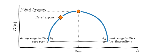
Figure 2: (color online) Schematic picture of the multifractal spectrum with the characteristic parameters: spectrum width, Hurst exponent and $h_{max}$ (the most probable singularity)

These values describe crucial properties for the recorded signals. The spectrum width determines the diversity of periods with the different scales (for high and low fluctuation). The values of Hurst exponent describe the nature of noise found in the time series. The range of the Hurst exponent values can be interpreted [15, 19, 6] as follows $h\in(0,0.5)$ indicates the antipercistency of the signals, $h=0.5$ represent an uncorrelated noise, $h\in(0.5,1)$ indicates the persistency of the series. This interpretation of the entire signal is valid only if the data exhibits the monofractal character. For the multifractal systems the set of the exponents is needed which is caused by the local character of the fluctuations. The shape of mf-spectrum itself has wide, meaningful interpretation [13, 19].

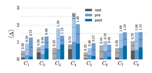
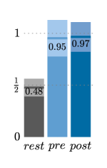
Figure 3: (color online) Mean values of the spectral width $\Delta$. Left panel: comparison of mean values for the individual groups of muscles (see text for details). Right panel: comparison of the mean values for three different states – at rest, before the training (pre) and after the training (post). Numbers refer to the actual values of means. The confidence interval is depicted with the slightly lightened colors for each bar separately.

4 Results

Despite many advantages offered by MFDFA method in the application to the complex biomedical data, some particular steps require from the users the individual decisions which can have significant impact on the final results. The main issue concerns the choice of the scaling range $s$ for the proper estimation of the fluctuation function $F_{q}(s)$ (4). In the literature one can find some useful advices for the appropriate selection the range of the scales [6, 19].

The length of the analysed time series $N$ consists of around $21000$ data points. For the calculations presented in this work the scales (segments length) $s\in(64,512)$ and typical $q\in(-5,5)$ were chosen. The examples of the double logarithmic dependence $F_{q}(s)$ vs $s$ together with the corresponding multifractal spectra are presented in the Fig. 4. Within the selected range of scales the linear dependence of the fluctuation function $F_{q}(s)$ on the segment length $s$ can be observed. Also it can be noticed that for the presented working states (before and after the training) the spectrum is relatively wide and there is no significant difference between the values of mf–spectrum width before and after training.

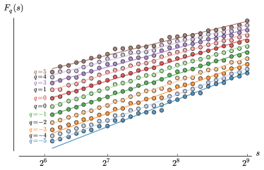
(a) $F_{q}(s)$ before training

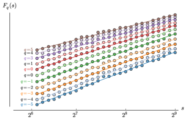
(b) $F_{q}(s)$ after training

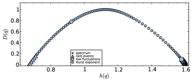
(c) mf–spectrum before training

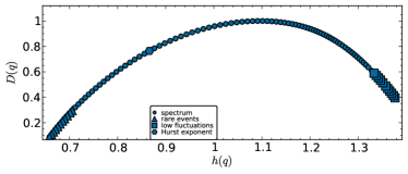
(d) mf–spectrum after training

Figure 4: The example of double logarithmic dependence $F_{q}(s)$ vs $s$ together with the corresponding multifractal spectra presented for the forearm muscle group from the right hand ($C_{6}$).

4.1 Spectrum width

The mean values of the spectral width are presented in the Tab. 1. Channels are assigned to each group of muscles. $C_{1}$–$C_{4}$ represent the left arm and $C_{5}$–$C_{8}$ indicate muscles from the right arm. $C_{1}$ and $C_{5}$ form a pair of the respective trapezius ridge group of muscles located on the left and right arms. Similarly the channels $C_{2}$ and $C_{6}$ record signals from the deltoids, $C_{3}$ and $C_{7}$ from the forearm muscle group (long palmar muscle and ulnar wrist flexor), and finally $C_{4}$ and $C_{8}$ from the group of thenar muscles.

Table 1: Mean values of the spectrum width for all channels and at each state.

Average spectrum width $\langle\Delta\rangle$
Channel number	$C_{1}$	$C_{2}$	$C_{3}$	$C_{4}$	$C_{5}$	$C_{6}$	$C_{7}$	$C_{8}$
Relaxation	0.3 $\pm 0.074$	0.564 $\pm 0.058$	0.35 $\pm 0.13$	0.743 $\pm 0.054$	0.233 $\pm 0.068$	0.441 $\pm 0.147$	0.39 $\pm 0.11$	0.794 $\pm 0.108$
Before training	0.58 $\pm 0.14$	0.577 $\pm 0.103$	1.204 $\pm 0.235$	1.865 $\pm 0.33$	0.465 $\pm 0.078$	0.778 $\pm 0.114$	1.095 $\pm 0.164$	1.063 $\pm 0.2$
After training	0.716 $\pm 0.216$	0.987 $\pm 0.14$	1.126 $\pm 0.1$	1.488 $\pm 0.22$	0.574 $\pm 0.15$	0.504 $\pm 0.14$	1.187 $\pm 0.155$	1.147 $\pm 0.174$

The smallest value of the spectrum width for each channel occurs at the relaxation state. The Wilcoxon test at the significance level of $\alpha=0.05$ was used in order to compare the relaxation state with the work states before and after the training. With the exception of $C_{5}$ and $C_{8}$ all other channels indicate a statistical significance at the selected level ($p<0.05$). This effect is clearly apparent in the right panel of Fig. 3 where the mean values of the mf–spectrum $\langle\Delta\rangle$ calculated from all the channels in the three states (rest, pre, post) are presented. The left diagram in Fig. 3 suggests the similar character of the spectrum width for the corresponding muscles in the right and left arms. For the series obtained before and after the training the highest value of the mf–spectrum width occurs for the groups of the forearm ($C_{3}$ and $C_{7}$) and thenar ($C_{4}$ and $C_{8}$) muscles, see Tab. 1 for details. The spectrum width can serve as an effective predictor for identification of the relaxation state of the muscle activity. On the other hand the width $\Delta$ alone cannot distinguish between the working states before and after the training.

4.2 Hurst exponent

The most important aspect of this work was the identification of the statistically different parameters which could be applied to distinguish between the signals obtained from the skilful and inexperienced student. This quantifiers could be than use for automatic evaluation of one’s ability of handling laparoscopic tools. Firstly we would like to focus on these two working states (pre and post) by means of the Hurst exponent $H$. In contrast to the just analysed width $\langle\Delta\rangle$, the mean Hurst exponent $\langle H\rangle$ indicates the statistical difference between of the data recorded before and after the training, c.f. Fig. 5. We grouped together the values for the corresponding clusters of muscles from the left and right arm for all six volunteers and calculated the arithmetic mean values of the Hurst exponent $\langle H\rangle$ for the corresponding channels separately. This values are summarized in the Table 2 and presented in the left panel of Fig. 5. For all the muscle groups the values of the Hurst exponent of the series after the training (post state) are significantly lower, see Fig. 5. The statistical significance occurs for deltoids ($C_{2}$ and $C_{6}$, with $p=0.0096$) and forearm ($C_{3}$ and $C_{7}$, with $p=0.0077$). The visual representation on this dependence is presented as the box plot in Fig. 6.

Table 2: Average values of the Hurst exponent $\langle H\rangle$ for the corresponding groups of muscles for the left ($C_{1}$–$C_{4}$) and right ($C_{5}$–$C_{8}$) hand at each of the three recorded states.

Average Hurst exponent $\langle H\rangle$
Muscles group	Trapezius ridge	Deltoid	Forearm	Thenar
	($C_{1}+C_{5}$)	($C_{2}+C_{6}$)	($C_{3}+C_{7}$)	($C_{4}+C_{8}$)
Relaxation/rest	$0.791\pm 0.071$	$0.894\pm 0.097$	$0.715\pm 0.055$	$1.304\pm 0.057$
Before training/pre	$0.868\pm 0.053$	$1.006\pm 0.035$	$0.853\pm 0.043$	$0.904\pm 0.067$
After training/post	$0.752\pm 0.042$	$0.811\pm 0.047$	$0.646\pm 0.0376$	$0.749\pm 0.06$

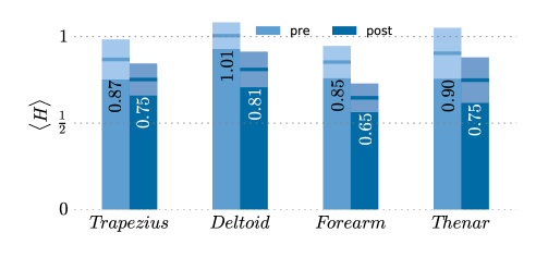
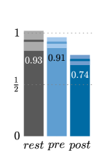
Figure 5: (color online) Mean values of the Hurst exponent. Left panel: comparison of mean values for the individual groups of muscles (see text for details). Right panel: comparison of the mean values for three different states – at rest, before the training (pre) and after the training (post). Bars indicate standard deviations. Numbers refer to the actual values of means. The confidence interval is depicted with the slightly lightened colors for each bar separately.

Figure 6: (color online) The box-and-whisker diagram of the average Hurst exponent $\langle H\rangle$ for two different groups of muscles at two different working states. The average Hurst exponents were calculated for both arms together. The plot for the forearm muscle group (long palmar muscle and ulnar wrist flexor) is shown on two diagrams on the l.h.s. The two diagrams on the r.h.s correspond to the deltoids. Pre and post reflects the abilities of using the laparoscopic tools before and after the training, respectively. The boxes correspond to the estimated quartiles and whiskers indicate a variability outside the upper and lower quartiles, i.e. the minimum and maximum values.

4.3 Thenar group of muscles

Upon the comparison of the signals acquired at rest and before the training sessions with those after the training the significant difference of the calculated averages of the Hurst exponents can be seen. This result is demonstrated in the right panel of the Fig. 5, where the mean values of Hurst exponent taken from the all the muscles together are presented for each of the states rest (gray), pre– (light blue) and post–training (blue). The dominant impact of this dissimilarity lies in the mean value of the Hurst exponent of the thenar muscles which show a statistically significant ($p=0.0037$) increase of the exponent for the relaxation state separately. This findings were quite unexpected as they indicate the different character of irregular component for the rest state of the discussed group of muscles alone. At the rest state the value is relatively high $\langle H\rangle_{C_{4},C_{5}}^{rest}=1.3037$ and is typically assigned to the integrated noise (random walk) [19]. For all the other muscle groups, the relaxation states show the persistence character [19], which is characteristic to the noisy nature of the time series, c.f. Tab. 2.

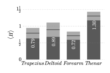
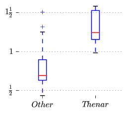
Figure 7: (color online) Average Hurst exponent presented for all group of muscles calculated for both arms together. The left panel shows bar chart for all of the groups separately. Please note that the thenar group of muscles possesses the highest, Brownian–motion–like, value of $\langle H\rangle$. All other groups can be interpreted as noisy signals. The confidence interval is depicted with the light grey for each bar separately. On the r.h.s. the box-and-whisker diagram of the average Hurst exponent is compared for joined groups of the trapezius, deltoid, and forearm muscles versus the thenar group. The boxes correspond to the estimated quartiles and whiskers indicate a variability outside the upper and lower quartiles, i.e. the minimum and maximum values.

The discussed cases are depicted in the Fig. 7 which compares the individual raw signals that indicate the biggest difference of the Hurst exponent at the relaxation state. Fig. 8 presents raw time series acquired from one of the volunteers from four groups of muscles left thenar, right thenar, left trapezius, right trapezius (top to bottom). The difference in the muscle activity – significantly lower amplitudes for the trapezius ridge and much larger fluctuations for the thenar group are clearly visible.

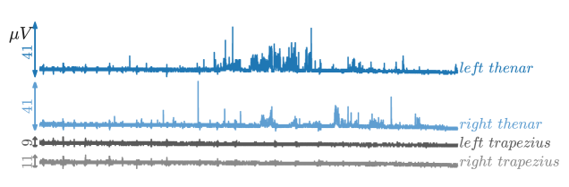
Figure 8: (color online) Exemplary raw sEMG signals acquired from one of the volunteers before the analysis. The arrows present the ranges of the recorded values of the signal in $\mu$V. Groups of muscles from top to bottom: left thenar, right thenar, left trapezius, right trapezius. The strong difference in the character of the signals can be notice just by the naked eye.

In addition, one can notice that for the thenar group the average spectral widths $\Delta$ also take the highest values out of all muscle groups (see Tab 1) for details).

This very muscle group exhibits several difficulties at the measurement. For instance the tools constantly touch the skin and can also touch the electrodes from time to time. This might cause an excessive sweating which in turn influence the signal. Last issue is the area of the electrodes in a relation to the area of the muscles. All of the above matter mainly at the work states, i.e. when the volunteer perform the actual task with the laparoscopic tools and are rather irrelevant for the rest state.

5 Conclusions

The signal from the surface electromyography recorded during the complex movements on the laparoscopic trainer was analysed. The main goal was to find a statistical difference between the signals acquired before (pre) and after (post) the training. In addition the relaxation (rest) state was considered. In order to quantify the complexity of the series the selected parameters which characterize a multifractal spectrum was used. The study of the spectral width does not allow to determine the differences in the pre–post states but is is sufficient to distinguish between rest and work states. Due to the small sample and also the necessity of using the non-parametric test, the statistical power of the test was respectively lower. However the investigation of the values of the Hurst exponent indicate that this parameter seems to be a better classifier between the analysed states (before and after the training) than multifractal spectrum width. For all of the examined muscle groups for both arms the values of the Hurst exponent appear to be lower after the series of training, however this difference is statistically significant only for the deltoid and forearm muscle groups. The rather unexpected findings is the character of the thenar muscles. Both the value of mf–spectrum width and the global Hurst exponent are distant from all other groups at the rest state. In a summary it can be concluded that surface electromyography indicates a potential method for the evaluation of complex dynamics of the action potential of the muscles. The research on the dynamical properties of the sEMG signals is still at early stage where many aspects are waiting to be discovered.

References

- [1] Aggarwal R, Moorthy K, Darzi A. Laparoscopic skills training and assessment. British Journal of Surgery. 2004;91(12):1549–1558.
- [2] Forsman M, Birch L, Zhang Q, Kadefors R. Motor unit recruitment in the trapezius muscle with special reference to coarse arm movements. Journal of Electromyography and Kinesiology. 2001;11(3):207–216.
- [3] Hug F. Can muscle coordination be precisely studied by surface electromyography? Journal of Electromyography and Kinesiology. 2011;21(1):1–12.
- [4] Merletti R, Parker PA. Electromyography: physiology, engineering, and non-invasive applications. vol. 11. John Wiley & Sons; 2004.
- [5] Barbero M, Merletti R, Rainoldi A. Atlas of muscle innervation zones: understanding surface electromyography and its applications. Springer Science & Business Media; 2012.
- [6] Gierałtowski J, Żebrowski J, Baranowski R. Multiscale multifractal analysis of heart rate variability recordings with a large number of occurrences of arrhythmia. Physical Review E. 2012;85(2):021915.
- [7] Goldberger AL. Non-linear dynamics for clinicians: chaos theory, fractals, and complexity at the bedside. The Lancet. 1996;347(9011):1312–1314.
- [8] Hampson KM, Mallen EA. Multifractal nature of ocular aberration dynamics of the human eye. Biomedical optics express. 2011;2(3):464–470.
- [9] Bryce R, Sprague K. Revisiting detrended fluctuation analysis. Scientific reports. 2012;2.
- [10] Chowdhury RH, Reaz MB, Ali MABM, Bakar AA, Chellappan K, Chang TG. Surface electromyography signal processing and classification techniques. Sensors. 2013;13(9):12431–12466.
- [11] Hakonen M, Piitulainen H, Visala A. Current state of digital signal processing in myoelectric interfaces and related applications. Biomedical Signal Processing and Control. 2015;18:334–359.
- [12] Goldberger AL, Rigney DR, West BJ. Chaos and fractals in human physiology. Sci Am. 1990;262(2):42–49.
- [13] Makowiec D, Gała R, Dudkowska A, Rynkiewicz A, Zwierz M, et al. Long-range dependencies in heart rate signals—revisited. Physica A: Statistical Mechanics and its Applications. 2006;369(2):632–644.
- [14] Konrad P. The abc of emg. A practical introduction to kinesiological electromyography. Noraxon, Scottsdale; 2005.
- [15] Kantelhardt JW, Zschiegner SA, Koscielny-Bunde E, Havlin S, Bunde A, Stanley HE. Multifractal detrended fluctuation analysis of nonstationary time series. Physica A: Statistical Mechanics and its Applications. 2002;316(1):87–114.
- [16] Kantelhardt JW. Fractal and multifractal time series. In: Encyclopedia of Complexity and Systems Science. Springer; 2009. p. 3754–3779.
- [17] Gupta V, Suryanarayanan S, Reddy NP. Fractal analysis of surface EMG signals from the biceps. International journal of medical informatics. 1997;45(3):185–192.
- [18] Ivanov PC, Amaral LAN, Goldberger AL, Havlin S, Rosenblum MG, Struzik ZR, et al. Multifractality in human heartbeat dynamics. Nature. 1999;399(6735):461–465.
- [19] Ihlen EA. Introduction to multifractal detrended fluctuation analysis in Matlab. Frontiers in physiology. 2012;3.
- [20] Lakhtakia A, Messier R, Varadan VV, Varadan VK. Self-similarity versus self-affinity: the Sierpinski gasket revisited. Journal of Physics A: Mathematical and General. 1986;19(16):L985.
- [21] Abry P, Gonçalves P, Lévy Véhel J. Scaling, Fractals and Wavelets. Digital signal and image processing series. London (UK): ISTE – John Wiley & Sons, Inc.; 2009.