The Riemann zeros as energy levels of a Dirac fermion
in a potential built from the prime numbers in Rindler spacetime
Abstract
We construct a Hamiltonian whose discrete spectrum contains, in a certain limit, the Riemann zeros. is derived from the action of a massless Dirac fermion living in a domain of Rindler spacetime, in 1+1 dimensions, that has a boundary given by the world line of a uniformly accelerated observer. The action contains a sum of delta function potentials that can be viewed as partially reflecting moving mirrors. An appropriate choice of the accelerations of the mirrors, provide primitive periodic orbits associated to the prime numbers , whose periods, measured by the observer’s clock, are . Acting on the chiral components of the fermion , becomes the Berry-Keating Hamiltonian , where is identified with the Rindler spatial coordinate and with the conjugate momentum. The delta function potentials give the matching conditions of the fermion wave functions on both sides of the mirrors. There is also a phase shift for the reflection of the fermions at the boundary where the observer sits. The eigenvalue problem is solved by transfer matrix methods in the limit where the reflection amplitudes become infinitesimally small. We find that for generic values of the spectrum is a continuum, where the Riemann zeros are missing, as in the adelic Connes model. However, for some values of , related to the phase of the zeta function, the Riemann zeros appear as discrete eigenvalues immersed in the continuum. We generalize this result to the zeros of Dirichlet -functions, associated to primitive characters, that are encoded in the reflection coefficients of the mirrors. Finally, we show that the Hamiltonian associated to the Riemann zeros belongs to class AIII, or chiral GUE, of Random Matrix Theory.
I Introduction
A century ago, Pólya and Hilbert suggested that the imaginary part of the non trivial zeros of the Riemann zeta function, would be the oscillation frequencies of a physical system. The reality of these frequencies will provide a proof of the celebrated Riemann hypothesis (RH) R59 which has deep consequences for the distribution of the prime numbers E74 -C03 . There are evidences that the Riemann zeros are the eigenvalues of a quantum Hamiltonian: i) the Montgomery-Odlykzo law according to which the statistical distribution of the zeros is given, locally, by the Gaussian Unitary Ensemble (GUE) of Random Matrix Theory (RMT) M74 -Me ; ii) analogies between trace formulas relating periods of classical trajectories and spectra in Quantum Chaos Theory and explicit formulas relating prime numbers and Riemann zeros B86 -B03 , and iii) Selberg’s trace formula relating the lengths of the geodesics on a compact Riemann surface with negative curvature and the eigenvalues of the Laplace-Beltrami operator S42 ; H76 . The picture proposed by Berry in 1986, is that the binomium primes/zeros is similar to the binomium classical/quantum for a dynamical chaotic system B86 . Furthermore, it was conjectured that the classical Hamiltonian underlying the Riemann zeros should be quasi-one dimensional, breaking time reversal symmetry and with isolated periodic orbits whose periods are the logarithm of the prime numbers (see K99 ; B03 for reviews of this approach, SH11 ; Wat for general references and MSa -DR for introductions and historical background).
In 1999 Berry and Keating (BK) BK99 ; BK99b , and Connes C99 , suggested that a spectral realization of the Riemann zeros could be achieved from the quantization of the simple classical Hamiltonian , where and are the position and momentum of a particle moving in the real line. The Hamiltonian is one dimensional, breaks the time reversal symmetry, is integrable, not chaotic, with unbounded classical trajectories and its quantization yields a continuum spectrum S07a ; TM07 . The connection found by Berry, Keating and Connes between and the Riemann zeros, was semiclassical, and relied on two different regularizations schemes. Berry and Keating introduced a Planck cell regularization of the phase space imposing the constraints and with , obtaining semiclassical energies that agree asymptotically with the average location of the Riemann zeros BK99 . In Connes’s work, there is a cutoff , and the constraints and , such that in the limit , the semiclassical spectrum becomes a continuum with missing spectral lines associated to the average Riemann zeros C99 . The interpretation of the zeros as missing spectral lines, would also explain a mysterious sign problem in the fluctuation term of the number of zeros C99 . The possible connection between and the Riemann zeros motivated several works in the past two decades, some of them will be discussed in more detail below A99 -N14 .
The previous semiclassical versions of were formulated as consistent quantum mechanical models in references ST08 ; SL11 ; S12 ; BK11 . Connes’s version was realized in terms of a charge particle moving in a box of size , and subject to the action of a uniform perpendicular magnetic field and an electrostatic potential ST08 . For strong magnetic fields the dynamics is restricted to the lowest Landau level, where the potential acts effectively as the quantum Hamiltonian. In this realization, the smooth part of the counting formula of the Riemann zeros appears as a shift of the energy levels (that become a continuum in the limit and not as an indication of missing spectral lines. The Landau model with potential, has been used in an analogue model of Hawking radiation in a quantum Hall fluid St13 .
On the other hand, the Berry-Keating version of was revisited recently using the classical Hamiltonian defined in the half line SL11 ; S12 (hereafter denoted as the model). The role of the term is to bound the classical trajectories which become periodic, unlike the trajectories of that are unbounded. The Hamiltonian can be quantized in terms of the operator , where and , and its spectrum agrees asymptotically with the average Riemann zeros provided . A similar result was obtained by Berry and Keating using the Hamiltonian that is invariant under the exchange BK11 . These two works provided an spectral realization of the average Riemann zeros, but not of the actual zeros. From the Quantum Chaos perspective, the reason of this failure lies in the fact that these variants of are non chaotic and does not contain periodic orbits related to the prime numbers BK11 . More generally, any one dimensional classical and conservative Hamiltonian is integrable and therefore non chaotic, which seems to lead to nowhere.
In this work we propose a solution of the puzzle that leads to a spectral realization of the Riemann zeros. The main ideas can be explained as follows. Let us consider a chaotic billiard in two spatial dimensions, such as the Sinai’s billiard S70 -St99 . A ball thrown with some energy follows chaotic trajectories that in most cases cover the entire table, except for a discrete set of periodic trajectories, whose periods, that are independent of the energy, dominate the path sum that gives rise to the Gutzwiller formula for the fluctuations of the energy levels. Unlike this, a one dimensional billiard, made of two walls, will be boring since the ball will go back and forth periodically between the walls.
Let us now take semitransparent walls, so that with a certain probability the ball passes through or bounces off. In such a billiard the particle may follow several trajectories depending on the outcome at each wall. One may say this is a quasi-one dimensional billiard. In Sinai’s billiard, or in the motion on compact Riemann surfaces, the particle follows geodesics, which implies that the periods of the closed orbits are independent of the energy. In the quasi-1D billiard, one can achieved the same property by choosing massless particles, say photons or massless fermions, whose trajectories lie on the light cone in Minkowsky space-time. The soft walls should then be viewed as semitransparent mirrors, or beam splitters.
The last ingredient one has to incorporate into the quasi-1D billiard, or rather the array of mirrors, is chaos. In table billiards, chaos is generated by a border that defocuses the trajectories, and in compact billiards, chaos is produced by the negative curvature of the space that separates nearby trajectories exponentially fast. If the 1D mirrors stay at fix positions, nearby light-ray trajectories will stay close in space-time. However, if the mirrors are accelerated, then slightly delayed light rays, will generally have their reflected rays departing exponentially fast from one another after several reflections. Hence in this model, the source of chaos is acceleration. The simplest situation is when the mirrors are uniformly accelerated, in which case they are called moving mirrors in the literature of Quantum Field Theory in curved spacetimes wil . We shall then consider an infinite array of moving mirrors whose accelerations, and reflection properties, will be used to encode number theoretical information. In particular, we shall choose the accelerations inversely proportional to a power of integers, that leads to the appearance of primitive periodic orbits whose periods are the logarithms of the prime numbers. These periods are measured by a moving observer whose acceleration sets the units of this magnitude.
This model realizes in a relativistic framework, Berry’s suggestion of associating primitive periodic orbits to prime numbers B86 . Quantum mechanically, the waves propagating in the array generate an interference pattern that encodes the accelerations and reflection coefficients of the mirrors. Here we find several situations: destructive interference where the Riemann zeros are missing spectral lines as in the adelic Connes’s model and constructive interference where the Riemann zeros are point like spectrum embedded in a continuum. In both cases, the connection between the spectrum of the model and the Riemann zeros involves a limit where the reflection amplitudes vanish asymptotically. This limit is analogue to the semiclassical limit , that leads to the Gutzwiller formula, that was the starting point of the analogies between Quantum Chaos and Number Theory.
The paper is organized as follows. In section II we review the basic definitions of Rindler spacetime that describes the geometry of the model. We formulate the massive Dirac fermion in a domain of the Rindler space-time, we find the Hamiltonian, study its relation with and recover the spectrum of the model, obtaining the interpretation of the parameters and as inverse acceleration and fermion mass. In section III we construct an ideal array of moving mirrors with accelerations and study the reflections of the light rays emitted and absorbed by an observer with acceleration . Using special relativity, we show that the proper time of the observer’s clock is proportional to , and that the choice singularizes the trajectories associated to the prime numbers. We also propose an array where , which has regular trajectories, and whose discrete spectrum is proportional to the integers (this model will be denoted harmonic). In section IV we construct the Hamiltonian of a massless Dirac fermion with delta function potentials associated to the moving mirrors of section III. We derive the matching conditions for the wave functions and show that the corresponding Hamiltonian is self-adjoint for generic values of the accelerations and the reflection coefficients. The eigenvalue problem for the Hamiltonian is formulated using transfer matrix methods, and in a semiclassical limit we find the conditions for the existence of discrete eigenvalues. In so far the construction is general, but then we analyze several examples and make contact with the Riemann zeta function and the Dirichlet functions. In section V, the identify the symmetry class of the Hamiltonian under time reversal (T), charge conjugation (C) and parity (P). In the conclusions we summarize our results and discuss future developments. In Appendix A we derive the spectrum of the harmonic model.
II The massive Dirac fermion in Rindler spacetime
II.1 Rindler spacetime
We start with some basic definitions and set up our conventions. The 1+1 dimensional Minkowski space-time is defined by a pair of coordinates , a flat metric , with signature , and line element
| (1) |
that is invariant under translations and Lorentz transformations (we set the units of the speed of light ). The change of coordinates,
| (2) |
brings (1) to the form
| (3) |
and are the Rindler space and time coordinates respectively R66 ; Gra . The Rindler metric (3) is invariant under shifts of , generated by the Killing vector . Restricting to positive values, defines the region called right Rindler wedge R66 -URMP ,
| (4) |
that in Minkowski coordinates is described by the quadrant . The value represents a horizon of the metric (3), that is similar to the horizon of a black hole, the reason being that the Schwarzschild metric, near the black hole horizon, is approximately the Rindler metric Gra .
Rindler spacetime is the natural arena to study the physical phenomena associated to accelerated observers R66 , such as the Unruh effect U76 ; URMP . Let us consider an observer whose world line is given by (2), with a constant value. The proper time, , measured by the observer is defined by , and its relation to follows from (3)
| (5) |
plus an additive constant that is set to 0 in (5). The observer’s trajectory (2), written in terms of its proper time, reads
| (6) |
and has a constant proper acceleration, , defined as the Minkowski norm of the vector
| (7) |
Restating the speed of light, . This quantity plays an central role in the Unruh effect according to which an observer, with proper acceleration , detects a thermal bath with temperature (in units ) U76 . Replacing by the surface gravity of an observer near the horizon of a black hole, yields the Hawking temperature H74 ; H75 . The similarity between the Hawking and Unruh formulas lies in the equivalence principle of General Relativity.
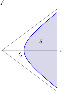
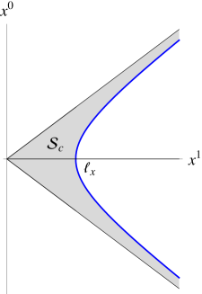
In our approach to a spectral realization of the Riemann zeros, we shall introduce an observer with acceleration, . The observer’s world line, , divides into the regions and located to her right and left,
| (8) | |||||
such that . Let us next study the dynamics of a Dirac fermion in .
II.2 Dirac fermion
A representation of the Dirac’s gamma matrices in 1+1 dimensions is given by yellow
| (9) |
where are the Pauli matrices. satisfy the Clifford algebra
| (10) |
In an abuse of notation, denotes the 1+1 analogue of the 1+3 gamma matrix , and it defines the chirality of the fermions. A Dirac fermion is a two component spinor
| (11) |
where are the conjugate of . The fields are the chiral components of , namely . Let us introduce the light cone coordinates , and the derivatives
| (12) | |||||
where the Minkowski metric (1) becomes . Under a Lorentz transformation with boost parameter , that is velocity , the light cone coordinates and the Dirac spinors transform as
| (13) |
and the Rindler coordinates as
| (14) |
Hence the spinors
| (15) |
remain invariant under (14). The spaces and are mapped into themselves under Lorenzt transformations.
II.3 Dirac action of a massive fermion
The Dirac action of a fermion with mass in the space-time domain is (units )
has a boundary corresponding to the worldline . The variational principle applied to (II.3) gives the Dirac equation
| (17) |
and the boundary condition
| (18) |
where is an infinitesimal variation of , is the Levi-Civita tensor , and is the tangent to in the Rindler coordinates (2). The Dirac equation (17) reads in components
| (19) |
In the massless case, the fields decouple and describe a right moving fermion, , and a left moving fermion, , in terms of which one can construct a Conformal Field Theory with central charge yellow . The mass term couples the two modes and therefore conformal invariance is lost. The action principle applied to the last expression of eq.(II.3) gives
| (20) |
and the boundary condition
| (21) |
Eqs.(20) and (21) are of course equivalent to (19) and (18) respectively. The infinitesimal generator of translations of the Rindler time , acting on the fermion wave functions, is the Rindler Hamiltonian , that can be read off from (20)
| (22) |
| (23) |
where , is the momentum operator associated to the radial coordinate . The operator
| (24) |
coincides with the quantization of the classical Hamiltonian proposed by Berry and Keating BK99 , where is the radial Rindler coordinate. The eigenfunctions of (24) are
| (25) |
with eigenvalues in the real numbers IR if S07a ; TM07 . Thus consists of two copies of , with different signs corresponding to opposite chiralities that are coupled by the mass term. In CFT the operator , with , corresponds to the sum of Virasoro operators that generate the dilation transformations.
II.4 Self-adjointess of
The action (II.3) is invariant under the transformation . The corresponding Noether current is , and is conserved, i.e. . The charge associated to can be integrated along the space-like line (2) with constant . Using (15) one finds
| (26) |
where are the complex conjugate of . Hence the scalar product of two wave functions, in the domain , can be defined as
| (27) |
The Hamiltonian is hermitean (or symmetric) respect to this scalar product if
| (28) |
when acting on a subspace of the total Hilbert space. Partial integration gives
| (29) |
Hence is hermitean provided
| (30) |
The latter condition is equivalent to eq.(21). The solution of (30) is
| (31) |
where . The quantity has the physical meaning of the phase shift produced by the reflection of the fermion with the boundary. It will play a very important role in what follows.
is not only hermitean but also self-adjoint. According to a theorem due to von Neumann, an operator is self-adjoint if the deficiency indices are equal vN ; GP90 . These indices are the number of linearly independent eigenfunctions of with positive and negative imaginary eigenvalues,
| (32) |
If , the operator is essentially self-adjoint, while if , then admits self-adjoint extensions. In the case of , one finds , and the self-adjoint extensions are parameterized by the phase in eq.(31).
II.5 Spectrum of
The eigenvalues and eigenvectors of the Hamiltonian (23), are given by the solutions of the Schroedinger equation
| (33) |
that satisfy the boundary condition (31). is the Rindler energy. The equations for that follows from (23) are
| (34) |
that lead to the second order differential eqs.
| (35) |
whose general solution is a linear combination of the modified Bessel functions AS72
| (36) |
The phases follows from (34). Let us compute the deficiency indices of , for which it is enough to take ,
| (39) | |||||
| (42) |
The functions diverge exponentially as , that forces , while decreases exponentially and are normalizable provided . The deficiency indices are therefore equal, and the eigenfunctions are (setting )
| (43) |
which yields
| (44) |
up to a common normalization constant. Plugging (44) into (31) yields the equation for the eigenenergies
| (45) |
This equation has positive and negative solutions, but only if or , they come in pairs . Moreover, if , then is also an eigenvalue. The imaginary part of the Riemann zeros also form pairs (i.e. ), and is not a zero since . This situation corresponds to the choice .
The number of eigenvalues, , in the interval (with ) is given in the asymptotic limit by
| (46) |
For there is a similar formula with . Let us compare this expression with the Riemann-Mangoldt formula that counts the number of zeros, , of the zeta function that lie in the rectangle E74
| (47) | |||||
where is the average term and the oscillation term. This expression agrees with (46), to order and , with the identifications
| (48) |
However, the constant term is not reproduced by eq.(46) for , which is the choice for the absence of the zero mode (note that neither gives the 7/8).
Comments:
-
•
In the limit , the spectrum (46) becomes a continuum. This situation arises in three cases: 1) if is kept constant and , the domain becomes , and one recovers the spectrum of a massive Dirac equation in ; 2) if is kept constant, and , the particles become massless and the effect of the boundary , is to exchange left and right moving fermions, that constitutes a boundary CFT yellow , and 3) and that corresponds to a massless fermion in .
-
•
Equation (45) coincides with the spectrum of the quantum Hamiltonian SL11 ; S12
(49) with the identifications
(50) The origin of this coincidence lies in the fact that a classical Hamiltonian of the form S12 can be formulated as a massive Dirac model in a space-time metric built from the potentials and MS12 . In the case of the model this metric is flat, which allows us to formulate this model in terms of the Dirac equation in the domain .
-
•
Gupta et al. proposed recently the Hamiltonian as a Dirac variant of the Hamiltonian G12 . The former Hamiltonian is defined in 2 spatial dimensions and after compactification of one coordinate becomes 1D, with an spectrum that depends on a regularization parameter and which is similar to the one found from the Landau theory with electrostatic potential ST08 .
-
•
Burnol has studied the causal propagation of a massive boson and a massive Dirac fermion in the Rindler right edge relating the scattering from the past light cone to the future light cone to the Hankel transform of zero order and suggesting a possible relation to the zeta function burnol .
II.6 General Dirac action
For later purposes we shall introduce the general relativistic invariant Dirac action in 1+1 dimensions
| (51) |
where, in addition to the mass term, there is a chiral interaction and a minimal coupling to a vector potential (). Moreover can be functions of the space-time position, in which case becomes a scalar potential and a pseudo scalar potential. We saw above that for a constant mass the action (II.3) can be restricted to the domain , preserving the invariance under shifts of the Rindler time . It is clear that if depends in , but not in , the action remains invariant under translations of , and that the Hamiltonian is equal to (23), with replaced by . The same happens with the term if . Concerning the vector potential, the action (51) is invariant provided
| (52) |
in which case (51) becomes
Using gauge transformations one can reduce the number of fields in (II.6). This issue will be consider below in a discrete realization of this model. The equations of motion derived from (II.6) are
| (54) |
and can be written as the Schroedinger equation (22) with Hamiltonian
that acts on the wave functions that satisfy the boundary condition (31).
In summary, we have shown in this section, that the spectrum of the Rindler Hamiltonian, in the domain agrees asymptotically with the average Riemann zeros, under the identifications (48). However, there is no trace of their fluctuations that depend on the zeta function on the critical line. This observation is no surprising since the prime numbers should be included into the model. In the next section we shall take a first step in that direction.
III Moving mirrors and prime numbers
Here we construct an ideal optical system, in Rindler space-time, that allows to distinguish prime numbers from composite. In the next section we shall give a concrete realization of this optical system in the Dirac model. The system consists of an infinite array of mirrors, labelled by the integers , that have the following properties:
-
•
The first mirror, , is perfect, while the remaining ones, , are one-way mirrors (beam splitters) that reflect and transmit the light rays partially. The light rays can be replaced by massless fermions.
-
•
The mirrors move in Minkowski space-time with uniform accelerations , with , such that .
-
•
At time , the mirrors are placed at the positions (units ).
-
•
The worldlines of the mirrors are contained in the domain , whose boundary corresponds to the first mirror, , such that .
-
•
An observer carries the first mirror, and sends and receives light rays whose departure and arrival times she measures with a clock.
-
•
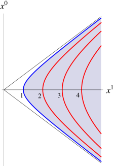
The lengths are given by
(58)
This ansatz can be replaced by ), but the parameter can be set to by scaling the clock’s ticks. Figure 2 depicts the mirror’s worldlines satisfying these conditions with .
We shall next study the propagation of light rays in this optical array using the laws of special relativity. Let us consider a light ray emanating from the point and reaching the point , where are the Rindler coordinates. Along this trajectory the line element (3) vanishes,
| (59) |
corresponding to right moving () or left moving () rays. Suppose that the ray is emitted at the first mirror at time , i.e. , moves rightwards, reflects on the nth mirror and returns to the first mirror, . The value of follows from eq.(59) and (58)
| (60) |
which is twice the change in from to . can be measured by the observer’s clock traveling with the perfect mirror where the ray was emitted and received. The change in the clock’s proper time is given by (see eq.(5)), which in units of , reads
| (61) |
Hence, measuring , the observer can find the value of . If , the ray travels forth and back between the mirrors and . However if , the ray must pass through the intermediate mirrors . Let us next analyze the case of two reflections. Now the ray is emitted at , reaches the mirror , returns to the perfect mirror, reflects again, reaches the mirror and comes back finally to the perfect mirror where the clock records the proper time, that is given by the sum of the intermediate times (61)
| (62) |
Hence the measurement of allows the observer to compute the product . There are more complicated cases as the one illustrated by the following sequence
| (63) | |||
where the ray emitted by the observer is reflected by the mirror , back to the mirror , that reflects the ray forwards to the mirror , that reflects the ray back to the first mirror. The proper time recorded by the clock is
| (64) |
Notice that the case reproduces eq.(62). It is easy to derive a general formula for the proper time elapsed for a trajectory involving intervals, that starts and ends at the first mirror,
| (65) | |||||
and is given by
| (66) |
The numerator of (66) corresponds to reflections: right mover left mover, while the denominator corresponds to reflections: left mover right mover. The argument of in (66) will be in general a rational number. Let us suppose it is the prime . It is clear, from (61), that after one reflection, i.e. , the observer will detect one ray arriving at . Suppose now that the argument of the log is a composite number , say . At time , the observer will detect the ray reflected from the forth mirror, but also one ray from two reflections on the second mirror , which is of course the same as . In a real experiment the two rays arriving at the observer will interfere. The study of this interference is left to the next section.
The previous example suggests that prime numbers correspond to unique paths characterized by observer proper times equal to . Let us prove this statement in the case . Equation (64) becomes
| (67) |
where satisfy the constraints (63). According to (67), divides the product , so it is a prime factor of or . In the former case one has
| (68) |
which is a contradiction because by eq.(63). The same result holds if divides . The generalization to any goes as follows. Suppose that , then from eq.(66)
| (69) |
If divides, say , one gets
| (70) |
which cannot be satisfied because by the conditions (65). This proves that the observer detects a single ray only when it comes from the reflection on a prime mirror, while it detects more than one ray when the rays comes from composite mirrors. This interpretation is purely classical because it presuposes that the rays can be distinguished, and disregards the interference effects. Both effects have of course to be taken into account in a realistic implementation using identical particles, such as photons or masless fermions. The interference pattern emerging for fermions in this array will be purpose of the next section. In any case, one can easily show that this classical model can be used to implement the classical Eratosthenes’s sieve to construct prime numbers.
Comments:
-
•
We mentioned in the introduction, that similarities between counting formulas in Number Theory and Quantum Chaos led Berry to conjecture the existence of a classical chaotic Hamiltonian whose primitive periodic orbits are labelled by the primes , with periods , and whose quantization will give the Riemann zeros as energy levels. A classical Hamiltonian with this property has not yet been constructed, but the mirror system presented above, displays some of its properties. In particular, the rays associated to prime numbers behave as primitive orbits with a period . Moreover, the trajectories and periods of these primitive rays are independent of their energy, that is the frequency of the light.
-
•
One can construct an array of moving mirrors in the domain (recall (8)) with the same properties as the array in . The parameters that characterize the array can be labeled with the negative integers,
(71) where is the perfect mirror located at the boundary . The proper time elapsed is now given by , and is identical to (61) . The relation between the arrays in and corresponds to the inversion transformation .
-
•
The array of mirrors defined in is an analogue computer for the multiplication operation or rather the addition of log’s. To implement the addition operation we shall define an array of mirror with positions, i.e. inverse accelerations,
(72) Where labels the perfect mirror. The analogue of eqs.(61) and (62) is (with )
(73) This is an harmonic array in the sense that the proper times (73), as well as the discrete spectrum (see Appendix A) are given by integer numbers. The harmonic array shows that it is not enough to have accelerated mirrors to generate chaos. The location/accelerations of the mirrors is essential. In the harmonic case, the exponential separation of the mirrors (72) compensates the exponential time dependence of the ray trajectories (59), that give rise to a tessellation of Rindler space-time. In the case of (58), the whole set of ray trajectories does not tessellate the Rindler spacetime which is a manifestation of the arithmetic chaos.
IV Massless Dirac fermion with delta function potentials
In this section we present a mathematical realization of the moving mirrors in the Dirac theory. We start from the massless Dirac action and represent the mirrors by delta function potentials that are obtained discretizing the interacting terms in the general action (II.6). The mass term becomes a contact interaction that turns left moving fermions into right moving ones, and viceversa. The new action remains invariant under translations in Rindler time, so that the Rindler Hamiltonian is a conserved quantity and we look for its spectrum using transfer matrix methods. The Dirac equation with delta function potentials requires a special treatment that we describe in detail (see SM81 -CNP97 for the Dirac equation with delta interactions in Minkowski coordinates).
IV.1 Discretization in Rindler variables
Let us consider the integral
| (74) |
where is a generic function, and is the radial part of the measure . The Rindler time can be easily incorporated into the equations. We shall discretize (74), using the positions of the mirrors given in eq.(58), which amounts to a partition of the half-line into segments of equal width , separated by the points
| (75) |
Let us discretize (74) as
| (76) |
If is a continuous function the last expression of (76) coincides with the middle one, but if is discontinuous one gets
| (77) |
where we used
| (78) | |||||
In the limit , the last expression in eq.(76) converges towards the integral (74) for well behaved functions. Replacing (75) into (76) yields
| (79) |
One could use this formula to discretize the mass term in the Dirac action (II.3). Taking this would yield
| (80) |
However, the corresponding Dirac equation is problematic, because the matching conditions are not consistent with the equations of motion, as shown in references SM81 -CNP97 . This problem is solved by replacing the local delta interactions by separable delta function potentials, that amounts to a point splitting. More concretely, the integral
| (81) |
should be replaced by
| (82) | |||
If and are continuous functions at , this expression is equivalent to (79).
IV.2 The Dirac action with delta function potentials
| (83) |
where is the massless action
| (84) |
and is the discretization of the mass terms and vector potential of (II.6) in the gauge
where
| (86) |
are dimensionless parameters that are equal to the values taken by the functions in (II.6) multiplied by . One can verify that the (83) is invariant under the scale transformation
| (87) |
so that the physical observables only depend on the parameters . In the Dirac model considered in the previous section, the mass is constant, which after discretization implies that . Later on we shall generalize this eq. to , and make contact with the Riemann zeta function .
IV.3 The Hamiltonian
The equations of motion that follows from (83) are
| (88) |
where (78) has been used to integrate around (to simplify the notation the variable has been suppressed). This equation implies that the left and right moving modes propagate freely and independently between the positions ,
| (89) |
Hence the Hamiltonian is (recall (23)),
| (90) |
The delta function terms yield the matching conditions between the wave functions on both sides of ,
| (91) |
that can be written in matrix form as
| (92) |
where is the two component vector (22) and
| (93) |
These matrices are invertible provided
| (94) |
Otherwise, eqs.(91) become a decoupled set of equations, hence from hereafter we shall assume that condition (94) is satisfied and leads to
| (95) |
where
| (96) | |||||
| (99) |
Finally, the variation of the action at the boundary gives the condition (31)
| (102) |
IV.4 Self-adjointness of the Hamiltonian
One should expect the Hamiltonian (90), acting on wave functions subject to the BC’s (95) and (102), to be self-adjoint. We shall next show that this is indeed the case. The scalar product, given by eq. (27), will be written as
| (103) |
To show that is a self-adjoint operator we follow the approach of Asorey et al. based on the consideration of the boundary conditions that turns out to be equivalent to the von Neumann theorem AIM05 . The starting point is the bilinear
| (104) |
where are two wave functions. This quantity measures the net flux or probability flowing across the boundary of the system, which for a unitary time evolution generated by must vanish. The self-adjoint extensions of select subspaces of the total Hilbert space where . In the case of the Hamiltonian (90) one finds
The term proportional to already cancels out by eq.(102). Imposing the independent cancellation of the terms proportional to yields
| (106) |
which we write as
| (107) |
where and . The general solution of (107) is obtained if and are related by a transformation
| (108) |
where satisfies
| (109) |
which implies that belongs to the Lie group . The non compact character of arises in this problem from to the relative minus sign of the terms in the Hamiltonian (90). The factor can be eliminated by a phase transformation of the field in the interval , which reduces the group to , that is
| (110) |
The matrices (96) are of this form, that ensures that is self-adjoint acting on the wave functions satisfying the conditions (95) and (102). One can further reduce the number of parameters in applying another transformation. Let us label the wave functions with an integer
| (111) |
and make the transformation
| (112) |
that induces the following changes in the boundary values
| (113) |
and in the matrices (recall (95))
| (114) |
The parameters can then be used to bring (96) into the form
| (117) |
corresponding to an element in the coset . We use the same notation for the transformed parameters as in (96).
IV.5 Eigenvalue problem
We shall now consider the eigenvalue problem of the Hamiltonian (90), acting on normalizable wave functions subject to the boundary conditions (95) and (102) The eigenfunctions of are given by
| (118) |
so for the interval (recall (111))
| (119) |
where will depend, in general, on the eigenenergy and is measured in units of (in what follows we take ). The phases have been introduced by analogy with the eigenfunctions (44). The values of on both sides of are given by
| (120) | |||||
Let us write these equations in matrix form in terms of the vector
| (121) |
and the matrix
| (122) |
such that (120) read
| (123) | |||||
Plugging these eqs. into the matching condition (95) yields
| (124) |
so
| (125) |
and substituting (117)
| (128) |
To simplify the notations let us define
| (129) |
so that
| (132) |
The parameters have the meaning of reflections amplitudes associated to the mirror. The absence of a mirror at the position is expressed by the condition , so that . Concerning the condition (102), equation (119) implies
| (133) |
that can be written as
| (134) |
Therefore, the eigenvalue problem has been reduced to find the energies for which the amplitudes , satisfying (125) and (134), yield wave functions (119) that are normalized in the discrete sense (Kronecker delta function) or in the continuous sense (Dirac delta function), corresponding to the discrete or continuum spectrum of the Hamiltonian. To this aim, we shall also need the norm and scalar product of the wave functions written in terms of the amplitudes. Using eq.(103), the norm of (119) is given by
| (135) |
and the scalar product of two eigenfunctions with energies and by
| (136) |
where and is the complex conjugate of . Since the Hamiltonian is self-adjoint this product will vanish.
IV.6 Semiclassical approximation
The recursion relation (125), together with the initial condition (134), gives all the vectors in terms of
| (137) |
Except for some simple cases, as the harmonic model (see Appendix A), it will impossible to find close analytic expressions of the product of matrices appearing in (137). The only hope to made progress is to evaluate (137) in the limit where the coefficients are infinitesimally small. We shall then assume that are proportional to a parameter that will be taken to zero at the end of the computation. This parameter plays the role of Planck’s constant, so the limit , will be interpreted as semiclassical. This interpretation is supported by the discretization of the massive Dirac equation, that led to eq.(86), according to which . The connection with the average Riemann zeros was achieved for , that corresponds in the semiclassical Berry-Keating model to the Planck constant .
Taking , the matrix given in eq.(132) can be replaced in the limit , by
| (140) |
can be expressed exactly as the exponential of a matrix of the form of , but in the limit , it will converge towards the expression given in (140) up to order . Plugging (140) into (137) yields
| (141) |
It is convenient to define a matrix , of order , corresponding to the choice of , which does not depend on because . The vector can be replaced by , where is equal to up to terms of order . Eq.(141) can then be written as
| (142) |
where has been replaced by since they become the same quantity in the limit . The product of exponentials of matrices can be approximated by the Baker-Campbell-Haussdorf formula GP90
| (143) |
that yields
| (144) |
Let us next define
| (145) |
where and are real for real values of . The factor 2 multiplying in eq.(140) can be absorbed into the parameter , so without loss of generality we can write
| (146) |
whose norm is
| (147) |
The discrete eigenvalues of the Hamiltonian are those for which the norm (135) is finite, which is ensured if (147) vanishes sufficiently fast when . The approximation we have performed above is a sort of inverse Trotter-Suzuki decomposition, e.g. , where a product of exponentials of non commuting operators is replaced by the exponential of their sum T59 ; S76 . Let us consider some examples.
IV.6.1 Harmonic model
This model is defined by the parameters (see eq.(72) with )
| (148) |
Let us remind that in this case the mirrors (delta functions) are labelled by , while the boundary is located at . can be positive or negative and is the semiclassical parameter. This model has an exact solution given in Appendix A, that allow us to verify the semiclassical approximation done below. From (145) one finds
| (151) |
In the case , one can choose and . This identification is not unique but simplifies the calculation. The norm (147) is given by
| (152) |
while the norm of the wave function , whose amplitudes are , reads (see eq. (135))
| (153) |
This series diverges for all values of different from and . This means that the energies , do not belong to the spectrum. On the other hand, if
| (154) |
the state has the norm
| (155) |
The parameter can be absorbed into the normalization constant of the state. Hence, in the two cases (154) there is an infinite number of normalized states with energies .
In the case , one can choose
| (156) |
The limit , yields and one recovers the previous result. If , eq.(156) shows that , hence the norm of will be bounded and the corresponding states will be normalizable in terms of Dirac delta functions, e.g. they belong to the continuum spectrum.
In summary, the spectrum of Hamiltonian of the harmonic model, in the limit , is given by the union of a continuum part, , and a discrete part, , where
| (157) | |||||
| (158) |
Note that in the case , the energies are missing in the continuum. For finite values of the spectrum is given by (see Appendix A)
| (159) |
where (see eq.(230)), so if the gap between the intervals closes and the continuum spectrum becomes , and the discrete spectrum as in (157). When , one also recovers the spectrum in (158).
Let us consider another example with the same values of but exponential decaying reflection amplitudes
| (160) |
that yields
| (161) |
If , one recovers eq.(151). Let us see if the discrete spectrum of the previous model survives when . Taking yields
| (162) |
Hence for any finite value of , the quantities are bounded, and therefore the state belongs to the continuum, e.g. the discrete spectrum disappears, but it can be recovered in the limit , where .
IV.6.2 Polylogarithm model
This model is defined by the parameters (see eq.(58) with )
| (163) |
The positivity conditions on and ensures that as , including the case where . The norm of the wave function is given by (see eq.(135))
| (164) |
so its convergence depends on the asymptotic behavior of . The ansatz (163) yields
| (165) |
that in limit becomes
| (166) |
where is the polylogarithm function wiki . In the limit there is the expansion
| (167) |
If , the term proportional to drops out and one is left with
| (168) |
which implies that the norm of converges towards a constant, for any value of , and therefore the series (164) diverges logarithmically signaling a continuum of states normalizable in the Dirac delta sense. If , the term proportional to dominates hence
| (169) |
leading to
| (170) |
If is kept fixed, the norm of is bounded and one gets again a continuum spectrum. Let us see what happens in the limit . Here , and therefore the norm of does not blow up, and actually converges to zero, if and only if
| (171) |
This result suggests that a regularized version of this model, involving the limit , should contain eigenstates satisfying (171). For , the Stirling formula provides the asymptotic behavior
| (172) |
that in the limit , becomes a continuum. The parameter regularizes the model and in some respects is analogue to the cutoff in Connes’s model, with . However, in eq.(172) the term , appears with an opposite sign as compared with Connes model, and it does not have the meaning of missing spectral lines, but rather of a finite energy correction. Notice also that if , the spectrum has the symmetry , provided if or if , like in the harmonic model analyzed above.
In summary, for the spectrum is a continuum related to the Riemann zeta function . This result is consistent with the studies carried by several authors in the past where the zeta function appears in connection to the scattering states of some physical system PF75 -J03 . However, for the connection with the zeta function is lost and only the smoothed zeros appear as a finite size correction to the level counting formula, in analogy with Connes’s version on the model, but with opposite sign. We are then forced to look for another ansatz for the reflection coefficients , if the zeros are to be realized as discrete eigenvalues of the Hamiltonian in the semiclassical limit. A hint is provided by the harmonic model, where the eigenvalues , arises from the blow up of as . This property leads us to the next example.
IV.6.3 Riemann model
The model is defined by the parameters
| (173) |
where is the Moebius function that vanishes if contains as divisor the square of a prime, and it is equal to 1 ( if is the product of an even (odd) number of distinct primes, that is Apostol
| (174) |
In this expression are different prime numbers. Integer numbers for which are called square free. The Moebius function has been used to construct an ideal gas of primons with fermionic statistics J90 ; S90 . In our model, appears in order to amplify the interference between waves so that the Riemann zeros are not swept out in the semiclassical limit and become visible. In the limit one finds
| (175) |
The case is equivalent to the Prime Number Theory, that was proved by Hadamard and de la Vallée-Poussin by showing that E74 . Repeating the analysis performed in the previous models, we find that for , the spectrum is given by IR . Indeed, for all values of , the norm of approaches a constant value in the limit , and consequently the norm (164) diverges logarithmically. The same thing occurs for , under the RH according to which this region will be free of zeros.
We are then left with the model with to provide a spectral realization of the zeros. Let us first approach this case in the limit when is a zero, that is . Expressing the zeta function on the critical line as , where and are the Riemann Siegel functions E74 one finds
| (176) |
where . For the sake of the argument we have assumed that is a simple zero of , a fact that is unknown to hold for all zeros. If that is the case, the sign of the derivative of at the zeros satisfy the rule
| (177) |
where the positive zeros are labelled as and the negative zeros as Equation (177) can be derived from the continuity of and the fact that . Plugging (176) and (177) into (175) gives
| (178) |
that leads to the choice
| (179) |
Hence the limit , implies , whereby the amplitude blows up unless the parameter satisfies
| (180) |
in which case , corresponding to a normalizable state. This is an important result that we shall derive more rigorously a bit later, but now let us discuss its implications.
-
•
The value of satisfying eq.(180) can be written as (with )
(181) where is the average number of zeros in the range (see eq.(47)). In the absence of fluctuations the average would be exact, that is , whereby . Hence a single value of would work for all the zeros. But the existence of fluctuations make things more interesting. To hear a given zero B12 one has to fine tune according to eq.(181), which pass to depend on the phase of the zeta function, . One thus obtains that the Riemann zeros and the phase of the zeta function both acquire a physical meaning in the model.
-
•
Berry B86 , and Badhuri et al. BKL95 have argued that a better approximation to the average zeros is obtained if
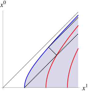
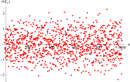
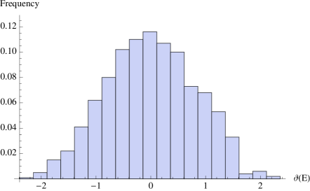
(182) This result can be visualized by plotting the real and imaginary parts of in the complex plane for a large interval of . One obtains a collection of loops that cut the real axis at the Gram points where , and that just before crossing the origin at , the loop cuts the imaginary axis, where . Badhuri et al. also show that gives roughly the scattering phase shift of a non relativistic particle in an inverted harmonic potential ( with a hard wall at the origin. Now, replacing (182) into (181) gives that in average . This result is confirmed in Fig. 3 which shows for the first zeros together with an histogram.
So far we have considered the value of , using eq.(175). To show the existence of discrete states for , we need the finite sum giving , that can be computed using the Perron’s formula Apostol ; Ba11
| (183) |
where means that the last term in the sum must be multiplied by 1/2 when is an integer. The integral (183) can be done by residue calculus Ba11
| (184) |
where the sum runs over the poles of located to the left of the line of integration, that is . For , the sum (183) is basically the Mertens functions that plays an important role in Number Theory E74 -D . Here we are interested in the values , with a real number. Eq.(183) imposes the condition . Hence the poles of that contribute to (184) have their real part smaller than , that is . The origin is a simple pole if and a multiple pole if . In the latter case we shall assume that is a simple zero so that the pole is double. The corresponding residues are given by
| (185) |
The remaining poles of come from the zeros of , except the case , that is included in (185). The trivial zeros of contribute with the poles , with residue
| (186) |
The non trivial zeros of , denoted as , contribute with the poles (note that ), with residue
| (187) |
Collecting results we find
| (188) | |||||
These equations are formally exact, so it would be interesting to prove them and find their range of validity. In what follows, we shall derive their consequences. Let us recall that the LHS of (188) gives essentially , where is to be identified with . Neglecting for a while the summands in these expressions one finds
| (189) | |||||
In the first case remains bounded in the limit , that would yield a state in the continuum. In the second case we choose
| (190) |
that can be compared with (179). Then imposing eq.(180), yields the asymptotic behavior of the norm of (see eq.(147))
| (191) |
and a wave function whose norm given by (164)
| (192) |
which is finite for any corresponding to a discrete eigenstate with energy .
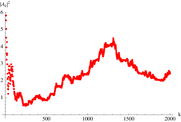
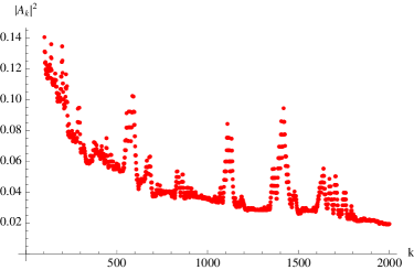
Fig. 4 shows in the case where corresponds to a state in the continuum, and for the first zero , corresponding to a discrete state. In the latter case we took , that guarantees that the norm converges to zero except for some jumps. For other values like the norm increases with . The same pattern is observed for other zeros. The values of are mostly concentrated around 0 (see Fig. 3). Finally, we have computed the norm of the vector , using eq.(164) observing that, for the zeros, it converges to a finite value with the choice (181), and diverges in the remaining cases. These results are in agreement with eq.(192).
Let us now return to the summands in eq.(188) that we neglected in the previous computation. The last term corresponding to the trivial zeros quickly converges to 0 as . The term associated to non trivial zeros on the critical line, , oscillates as , and we expect that it gives subleading contributions to the main term that goes with . Finally, a zero off the critical line, say , would give a contribution , that dominates over the remaining terms, for all values of , leading to
| (193) |
where and do not depend on . The expression of diverges when , but unlike the case of (190), the phase cannot be fixed to a value that cancels the divergent term in the norm (147). Hence , would grow typically as , so that the wave function will not be normalizable even in the continuum sense. This occurs for any value of , so we arrive at the paradoxical conclusion that a zero off the critical line implies that the Hamiltonian does not have eigenstates !! That’s not certainly the case because is a well defined self-adjoint operator, so we must conclude that off critical zeros do not exist. This result seems to provide a proof of the Riemann hypothesis, but one must be very cautious since it relies on several unproven assumptions.
Comments:
-
•
In the spectral realization proposed above there cannot exist zeros outside the critical line in the form of resonances. As explained above, their presence leads to the non existence of eigenvectors of the Hamiltonian .
-
•
von Neumann and Wigner showed that in ordinary Quantum Mechanics it is possible to have a bound state immersed in the continuum VW29 ; GP90 . They used a potential that decays as with oscillations that trap the particle thanks to interference effects. There is a general class of models with this property S69 -CH02 , and they all require a fine tuning of couplings. That this phenomena may happen for the Riemann zeros was suggested in S07a using a model with non local interactions.
-
•
The delta function potential needed to reproduce the zeros depends on the Moebius function that exhibits an almost random behavior. This result is reminiscent of the fractal structure of the quantum mechanical potentials built to reproduce the lowest values of prime numbers and the Riemann zeros. The latter potentials were built from the smooth ones obtained by Mussardo, for the primes M97 , and Wu and Sprung, for the zeros WS , and have a fractal dimension around 2 and 1.5 respectively R95 -SBH08 .
IV.6.4 Dirichlet model
We shall briefly describe how the previous results can be generalized to Dirichlet functions. These are analytic functions constructed from a Dirichlet character as D
| (194) |
where the product runs over the prime numbers (Euler formula). A character of modulus , is an arithmetic function satisfying if divides D . One has that or 0, and if , the character is called real. The number of characters with modulus is given by the Euler totient function , that counts the number of coprime divisors of . For , the character is , that corresponds to the Riemann zeta function . Primitive characters are those that cannot be written as products of characters of smaller modulus , and can be classified into even or odd if respectively.
The -functions associated to primitive characters satisfy the functional relation
| (195) |
where for an even (odd) character, is the character conjugate to , e.g. , and is the Gauss sum
| (196) |
On the critical line , eq.(195) reads
| (197) |
For real it is useful to parameterize the functions as
| (198) |
where is real and is a phase that can be found from eq.(197)
| (199) |
coincides with when is the identity character. For real characters, the zeros of , appear symmetrically, , that is reflected in the properties, and . However for complex characters this symmetry is broken.
The Dirac model associated to will be defined by the parameters
| (200) |
Note that one can deal with complex characters thanks to the existence of two types of mass terms, and . The characters acquire a physical meaning related to the reflection coefficient of the mirror. This provides a unified framework to deal with the whole family of Dirichlet -functions.
We can repeat the analysis done for the zeta function to find the discrete eigenenergies in the spectrum. For example, the asymptotic limit of is given by
| (201) |
which shows that the zeros of appear as poles of , that lead eventually to discrete states, provided is fine tuned appropriately. Assuming that the zeros of are simple, the value of for which is a discrete state is given by
| (202) |
For the zeta function, , eq.(181) is recovered from (202). We expect the zeros of the Dirichlet functions, associated to primitive characters, to form the discrete spectrum of the corresponding Hamiltonians. That would amount to a proof of the Generalized Riemann hypothesis.
V CPT symmetries and AZ classes
The statistical properties of the Riemann zeros, conjectured by Montgomery and confirmed numerically by Odlyzko, have been one of the main motivations to search for a spectral origin of these numbers. The conjecture is that the zeros satisfy, locally, the GUE law, which implies that the Riemann dynamics breaks the time reversal symmetry. Deviations from the GUE law were later on identified by Berry and collaborators, as a trace of the semiclassical origin of the zeros and a breakdown of universality. It is thus of great interest to study the discrete CPT symmetries and RMT universality classes of the Hamiltonians discussed in previous sections.
The action of the time reversal symmetry (), charge conjugation or particle-hole symmetry (), and parity or chirality () on a vector are defined as BL1 ; BL2
| (203) |
where are unitary matrices, i.e. and is the complex conjugate of . Here is the column vector formed by the coefficients of a pure state of a Hilbert space in an orthonormal basis. and are antiunitary transformations and is unitary. A Hamiltonian has or symmetry if it satisfies the conditions
| (204) |
Since is hermitean, , then the symmetry becomes . Notice that is the product of and , and one can choose . There is a basis where and are real, and symmetric or antisymmetric matrices, i.e. and , in which case unitarity implies and . If a symmetry is broken, say , one writes . Counting all the possibilities one arrives to ten symmetry classes, as found by Altland and Zirnbauer (AZ), that include the classical Wigner-Dyson gaussian ensembles: GOE, GUE, and GSE as well as their chiral versions chGOE, chGUE, chGSE AZ . Among the 10 AZ classes there are 4 that break time reversal symmetry, which are the candidates to describe the zeros of and other -functions (see Table 1).
| AZ | Top | |||
|---|---|---|---|---|
| A | 0 | 0 | 0 | 0 |
| AIII | 0 | 0 | 1 | ZZ |
| D | 0 | 1 | 0 | |
| C | 0 | -1 | 0 | 0 |
Table 1.- The AZ classes where the time reversal symmetry is broken. Column ”Top” denotes the topological invariants of the class in one spatial dimension.
Let us review briefly the main properties of the classes of Table 1 and their relations with the problem at hand. Class characterizes Hamiltonians of the form , where is an hermitean matrix, with no further conditions placed on it. The statistical properties of random matrices of this form are described by GUE. As shown in Table 1, all the CPT symmetries are broken and there is no topological invariant in 1D.
Class D characterizes Hamiltonians of the form , where is imaginary and antisymmetric. The eigenvalues of appear in pairs , and if the dimension of the matrix is odd there is a zero eigenvalue. The Berry-Keating Hamiltonian belongs to this class, since here and S11b . The Hamiltonian also belongs to class provided the parameter , that characterizes its self-adjoint extensions, is or . The latter choices ensure that the eigenvalues of come in pairs , and that if , then is eigenvalue SL11 ; S12 . We can thus identify as the topological invariant of class in 1D.
Class C characterizes Hamiltonians of the form , where , and are the Pauli matrices that act in an additional 2 dimensional Hilbert space, that can be seen as a spin 1/2 S11b . Here , so . The eigenvalues of come in pairs , as in class . Srednicki proposed recently that class is associated to the zeros of the Dirichlet -functions whose characters are real and even, that includes the zeta function S11b . He was led to this proposal by a conjecture due to Katz and Sarnak KS99 according to which these -functions form a family related by a sort of symplectic symmetry, and by the fact that the spacings of their zeros agree asymptotically with the GUE distribution.
Class AIII, is a chiral version of GUE (chGUE) and characterizes Hamiltonians with the block structure
| (205) |
where is a complex matrix and the chiral operator. The eigenvalues of come in pairs . If is a matrix of dimension , then the number of zeros eigenvalues is that explains the Z Z topological invariant of this class. Class chGUE, together with its relatives chGOE and chGSE, describe massless Dirac fermions and have been applied to study the QCD Dirac operator, partition functions, etc VW -FS02 .
Let us next study the symmetry classes of the Rindler Hamiltonians constructed in previous sections. First of all, the massless Hamiltonian
| (206) |
admits different representations of the symmetries BL2 . Indeed, and can be realized as or , and as or . Adding a mass term to (206) selects a particular realization, e.g.
| (207) |
This Hamiltonian acts on the wave functions satisfying the BC (31). One can verify that this BC preserves , for all values of , however the symmetry is preserved only if . Hence in these two cases, the Hamiltonian (207) belongs to class BDI (chGOE) since . We mentioned in section II.E that the Hamiltonian ( see eq. (49)) has the same spectrum as (207) with the identifications (50). We show above that the former Hamiltonian belongs to class D, while we have found now that (207) belongs to class chGOE. There is no contradiction between these results. In both cases the symmetry explains the pairing of energies , while the symmetry appears from the doubling of degrees of freedom in the Dirac model.
Finally, let us show that the Dirac model associated to the Riemann zeros belongs to class AIII, with chiral operator . First of all notice that the matching conditions (95) are preserved by the action of , because in this model , and then
| (208) |
On the other hand, if is the eigenfunction with energy it satisfies the BC (102)
| (209) |
where . The function , given in eq.(181) for , satisfies that which, together with the equation , implies that if is an eigenstate with energy , then is an eigenstate with energy . Hence the pairing of energies is explained by the chiral symmetry and not by the charge conjugation symmetry as the Hamiltonian (207). One can perform a change of basis that brings the chiral operator and the Hamiltonian (206) into the form (205), with that is a real and antisymmetric matrix in some orthonormal basis. The Hamiltonian we are dealing with is therefore a subclass within the class chGUE.
VI Conclusions
We have proposed in this paper that a combination of Quantum Mechanics and Relativity Theory is the key to the spectral realization of the Riemann zeros. The old message of Pólya and Hilbert was that Quantum Mechanics should play a central role in this realization, an idea that is behind the successful applications of RMT, and Quantum Chaos, to Number Theory. What is new is that Einstein’s theory of Relativity must also be present. The reason is that the properties of accelerated objects, in Minkowski space-time, can be used to encode and process arithmetic information. In some sense, spacetime becomes an analogue computer, or simulator, that allows an accelerated observer to multiply numbers, and distinguish primes from composite, by measuring the proper times of events involving massless particles. In this way the prime numbers acquire a classical relativistic meaning associated to primitive trajectories of particles, along the lines suggested by the periodic orbit theory in Quantum Chaos.
The combination of Quantum Mechanics and Relativity is of course a Relativistic Quantum Field Theory, that in our case is the Dirac theory of fermions in Rindler space-time, the latter being the geometry associated to moving observers. The time evolution in this space is generated by the Rindler Hamiltonian that coincides with the Berry-Keating Hamiltonian , each sign corresponding to the chirality of the fermion. This operator is also the generator of dilations of the Rindler radial coordinate , but in the presence of delta function potentials, associated to the prime numbers, scale invariance is broken. This has the dramatic effect that the spectrum is a continuum, where the Riemann zeros are missing, in analogy with the result found by Connes in the adelic approach to the RH. However, the moving observer can fine tune the phase factor of the reflection of the fermion at the boundary, in such a way that a bound state appears with an energy given by a Riemann zero. The phase factor at the boundary is given essentially by the phase of the zeta function at the corresponding zero. This result is obtained in a limit where the perturbation of the massless Dirac action by the delta potential is infinitesimally small, so that the bound state is immersed in a continuum of states. This weak coupling limit is reminiscent to the semiclassical limit that leads to the Gutzwiller formula for the fluctuations of the energy levels in chaotic systems. The previous scenario leads to a proof of the Riemann hypothesis but more work is required to fully support this claim.
The present work suggests the possibility of an experimental observation of the Riemann zeros as energy levels. The system proposed here does not look realistic at the moment, but there are theoretical proposals to realize the Rindler geometry using cold atoms and optical lattices Latorre1 ; Javi . Another possible route is to use the Quantum Hall effect where arises as an effective low-energy Hamiltonian ST08 ; St13 . On a more theoretical perspective, this work points towards a relation between Riemann zeros and black holes, whose near horizon geometry is in fact Rindler G . The role played by the privileged observer in our construction reminds the brick wall model introduced by ’t Hooft to regularize the horizon of a black hole H85 . Throughout this paper the prime numbers have been treated as classical objects. However, they turn into quantum objects in the Prime state formed by the superposition of primes in the computational basis of a quantum computer LS1 ; LS2 . This poses the question whether the Prime state could be created with the same tools as the Riemann zeros become energy levels.
Acknowledgements.- I am very grateful for suggestions, and conversations to José Ignacio Latorre, Belén Paredes, Paul Townsend, Michael Berry, Jon Keating, Javier Rodríguez-Laguna, Manuel Asorey, Jose Luis Fernández Barbón, Giuseppe Mussardo, André LeClair, Mark Srednicki, Javier Molina, Luis Joaquín Boya and Miguel Angel Martín-Delgado. This work has been financed by the Ministerio de Ciencia e Innovación, Spain (grant FIS2012- 33642), Comunidad de Madrid (grant QUITEMAD) and the Severo Ochoa Program.
Appendix A The harmonic model
We first discuss some general properties of the transfer matrix that will be used later on to derive the exact spectrum of the harmonic model. Let us consider the transfer matrix (132), with , and the condition . It is easy to see that can be written as
| (210) |
where are the eigenvalues of (positive from the condition )
| (211) | |||||
and
| (212) |
Replacing (210) into (125) gives the recursion relation
| (213) |
We now define the vector
| (214) |
that satisfies
| (215) |
where
| (216) |
Notice that
| (217) |
Eq.(215), gives an alternative way to solve the eigenvalue problem that admits an interesting physical interpretation as the evolution of a kicked rotator with spin 1/2 St99 . In this interpretation the term represents the rotation of the spin around the -axis, with an energy during a time elapse , after which the spin is kicked with an imaginary magnetic field with strength along the -direction. Kicked rotators of this sort are currently employed to analyze quantum chaos in simple situations St99 .
Let us next consider the harmonic model defined by eq.(148), that according to eqs.(211, 216) correspond to constant values of and
| (218) |
In this case the recursion relation (215) can be iterated yielding
| (219) |
where the matrix is given by
| (220) |
Making the replacement , the matrix changes by an overall sign, which in turn implies that the spectrum has a periodicity. Let us consider the case where , that yields
| (221) |
which is convergent only in the following two cases
| (224) | |||||
| (227) |
These are normalizable eigenstates for all values of the coupling constant , even in the limit . Normalizable states for are also possible. The relation between the energy, , and is given by
| (228) |
that in the limit gives the discrete eigenvalues . Plugging in (228) we recover the cases (224). The continuum spectrum of the model can be derived from the condition that is an elliptic matrix (note that )
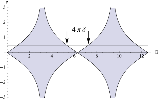
| (229) |
and consists of energy bands separated by a gap that are shown in Fig. 5
| (230) |
In the limit , the gap closes, and the discrete energy states become immersed in the continuum IR .
References
- (1) B. Riemann, ”On the number of primes less than a given magnitude”, translated by H. M. Edwards from ”Ueber die Anzahl der Primzahlen unter einer gegebenen Grösse” (1859) in E74 .
- (2) H.M. Edwards, Riemann’s Zeta Function, Academic Press, New York, 1974.
- (3) E.C. Titchmarsh, The Theory of the Riemann Zeta Function, Oxford Univ. Press, Oxford, 1986.
- (4) H. Davenport, Multiplicative Number Theory, Grad. Texts in Math., vol. 74, Springer-Verlag, New York, 2000.
- (5) E. Bombieri, Problems of the Millennium: The Riemann Hypothesis, Clay Mathematics Institute, (2000).
- (6) P. Sarnak, Problems of the Millennium: The Riemann Hypothesis, Clay Mathematics Institute, (2004).
- (7) B. Conrey, ”The Riemann Hypothesis , Notices of AMS, March, 341 (2003).
- (8) H.L. Montgomery, ”Distribution of the zeros of the Riemann zeta function”, in Proceedings Int. Cong. Math. Vancouver 1974, Vol. I, Canad. Math. Congress, Montreal, 379 (1975).
- (9) A.M. Odlyzko, ”Supercomputers and the Riemann zeta function”, in Supercomputing 89: Su- percomputing Structures & Computations, Proc. 4-th Intern. Conf. on Supercomputing, In- ternational Supercomputing Institute, St. Petersburg, FL, 348 (1989).
- (10) A. M. Odlyzko, The 1020-th zero of the Riemann Zeta Function and 70 Million of its Neighbors, www.dtc.umn.edu/?odlyzko/unpublished.
- (11) Bohigas and M. J. Gianonni, in Mathematical and Computational Methods in Nuclear Physics, edited H. Araki, J. Ehlers, K. Hepp, R. Kippenhahn, H. Weidenmuller and J. Zittart (Springer Verlag, Berlin, 1984).
- (12) M. L. Mehta, Random Matrices, Elsevier Ltd. The Netherlands, 2004.
- (13) M. V. Berry, “Riemann’s zeta function: a model for quantum chaos?”, in Quantum Chaos and Statistical Nuclear Physics, edited by T. H. Seligman and H. Nishioka, Springer Lecture Notes in Physics Vol. 263 , p. 1, Springer, New York (1986).
- (14) E. Bombieri, “Prime territory: exploring the infinite landscape at the base of the number system”, The Sciences 32, 30 (1992).
- (15) M. C. Gutzwiller, Chaos in Classical and Quantum Mechanics, Springer Verlag, New York, 1990.
- (16) J. P. Keating, ”Periodic orbits, spectral statistics and the Riemann zeros”, in Supersymmetry and Trace Formulae: Chaos and Disorder, eds. I.V. Lerner, J.P. Keating & D.E Khmelnitskii (Plenum Press), 1-15 (1999).
- (17) P. Leboeuf, A. G. Monastra, O. Bohigas, ”The Riemannium”, Reg. Chaot. Dyn. 6, 205 (2001); arXiv:nlin/0101014.
- (18) E. Bogomolny, ”Quantum and Arithmetical Chaos”, in Frontiers in Number Theory, Physics and Geometry, Les Houches, 2003; arXiv:nlin/0312061
- (19) A. Selberg, ”Harmonic analysis and discontinuous groups in weakly symmetric Riemannian spaces with applications to Dirichlet series”, Journal of the Indian Mathematical Society 20, 47 (1956).
- (20) D. A. Hejhal, ”The Selberg trace formula for ”., vol. 548 of Lecture Notes in Mathematics, Springer- Verlag (1976).
- (21) D. Schumayer, D. A. W. Hutchinson, ”Physics of the Riemann Hypothesis”, Rev. Mod. Phys. 83, 307 (2011); arXiv:1101.3116.
- (22) M. Watkins, Number Theory and Physics arxiv: http://empslocal.ex.ac.uk/people/staff/mrwatkin//zeta/physics.htm
- (23) M. du Satoy, The Music of the Primes, Harper Collins, NewYork (2003).
- (24) K. Sabbagh, Dr. Riemann’s zeros, Atlantic books, London (2003).
- (25) J. Derbyshire, Prime obsession, A plume book, New York (2003).
- (26) D. Rockmore, Stalking the Riemann hypothesis, Jonathan Cape, London (2005).
- (27) M.V. Berry, J.P. Keating, “ and the Riemann zeros”, in Supersymmetry and Trace Formulae: Chaos and Disorder, ed. J.P. Keating, D.E. Khmelnitskii and I. V. Lerner, Kluwer, 1999.
- (28) M. V. Berry, J. P. Keating, “The Riemann zeros and eigenvalue asymptotics”, SIAM Review 41, 236, 1999.
- (29) A. Connes, “Trace formula in noncommutative geometry and the zeros of the Riemann zeta function”, Selecta Mathematica New Series 5 29, (1999); math.NT/9811068.
- (30) B. Aneva, ”Symmetry of the Riemann operator”, Phys. Lett. B 450, 388 (1999).
- (31) G. Sierra, ”The Riemann zeros and the cyclic renormalization group”, J. Stat. Mech.: Theor. Exp. (2005) P12006; math.NT/0510572.
- (32) G. Sierra, ” with interaction and the Riemann zeros”, Nucl. Phys. B 776, 327 (2007); math-ph/0702034.
- (33) J. Twamley and G. J. Milburn, ”The quantum Mellin transform”, New J. Phys. 8, 328 (2006); quant-ph/0702107.
- (34) G. Sierra, ”Quantum reconstruction of the Riemann zeta function”, J. Phys. A: Math. Theor. 40 (2007) 1; math-ph/0711.1063.
- (35) G. Sierra, ”A quantum mechanical model of the Riemann zeros”, New J. Phys. 10, 033016 (2008); arXiv:0712.0705.
- (36) J. C. Lagarias, ”The Schroëdinger operator with Morse potential on the right half line”, Communications in Number Theory and Physics 3 (2009), 323; arXiv:0712.3238.
- (37) J-F. Burnol, ”On some bound and scattering states associated with the cosine kernel”, arXiv:0801.0530.
- (38) G. Sierra and P.K. Townsend, ”The Landau model and the Riemann zeros”, Phys. Rev. Lett. 101, 110201 (2008); arXiv:0805.4079.
- (39) S. Endres and F. Steiner, ”The Berry-Keating operator on and on compact quantum graphs with general self-adjoint realizations”, J. Phys. A: Math. Theor. 43, 095204 (2010); arXiv:0912.3183.
- (40) G. Regniers and J. Van der Jeugt, ”The Hamiltonian and classification of representations”, Workshop Lie Theory and Its Applications in Physics VIII (Varna, 2009); arXiv:1001.1285.
- (41) G. Sierra, ”A Physics pathway to the Riemann hypothesis”, Eds M. Asorey, et al. J. Vicente García Esteve, M. F. Rañada, J. Sesma, Prensas Univ. Zaragoza, Spain (2009); arXiv:1012.4264.
- (42) E. de Rafael, “Large-Nc QCD, Harmonic Sums and the Riemann Zeros”, Nucl. Phys. Proc. Suppl. 207, 290 (2010); arXiv:1010.4657.
- (43) G. Sierra and J. Rodríguez-Laguna, ”The model revisited and the Riemann zeros”. Phys. Rev. Lett. 106, 200201 (2011); arXiv:1102.5356
- (44) G. Sierra, ”General covariant models and the Riemann zeros”, J. Phys. A: Math. Theor. 45 055209 (2012); arXiv:1110.3203.
- (45) M. Srednicki, ”The Berry-Keating Hamiltonian and the Local Riemann Hypothesis”, J. Phys. A: Math. Theor. 44 305202 (2011); arXiv:1104.1850.
- (46) M. Srednicki, ”Nonclasssical Degrees of Freedom in the Riemann Hamiltonian”, Phys. Rev. Lett. 107, 100201 (2011); arXiv:1105.2342.
- (47) M. V. Berry and J. P. Keating, ”A compact hamiltonian with the same asymptotic mean spectral density as the Riemann zeros”, J. Phys. A: Math. Theor. 44, 285203 (2011).
- (48) K. S. Gupta, E. Harikumar and A. R. de Queiroz, ”A Dirac type xp-Model and the Riemann Zeros”, Eur. Phys. Lett. 102 10006 (2013); arXiv:1205.6755.
- (49) J. Molina-Vilaplana and G. Sierra, ”An model on spacetime”, Nucl. Phys. B 877, 107 (2013); arXiv:1212.2436.
- (50) R. V. Ramos and F. V. Mendes, “Riemannian Quantum Circuit”, Phys. Lett. A 378, 1346 (2013) arXiv:1305.3759.
- (51) J. C. Andrade, “Hilbert-Pólya conjecture, zeta-functions and bosonic quantum field theories”, Int. J. Mod.Phys. A28, 1350072 (2013); arXiv:1305.3342.
- (52) J. Kuipers, Q. Hummel and K. Richter, ”Quantum graphs whose spectra mimic the zeros of the Riemann zeta function”, Phys. Rev. Lett 112, 070406 (2014); arXiv:1307.6055.
- (53) M. C. Nucci, ”Spectral realization of the Riemann zeros by quantizing : the Lie-Noether symmetry approach”, Journal of Physics: Conference Series 482, 012032 (2014).
- (54) M. Stone, ”An analogue of Hawking radiation in the quantum Hall effect”, Class. Quantum Grav. 30, 085003 (2013); arXiv:1209.2317.
- (55) Ya. G. Sinai, ”Dynamical systems with elastic reflections”, Russ. Math. Surv. 25, 137, (1970).
- (56) M. V. Berry, ”Quantizing a Clasically Ergodic system: Sinai’s billiard and the KKR method”, Annals of Physics, 131, 163 (1981).
- (57) O. Bohigas, M. J. Giannoni and C. Schmit, ”Characterization of Chaotic Quantum Spectra and Universality of Level Fluctuation Laws”, Phys. Rev. Lett. 52, 1 (1984).
- (58) H.J. Stöckmann, Quantum Chaos: an introduction, Cambridge University Press, Cambridge, 1999.
- (59) C. Holzhey, F. Larsen and F. Wilczek, ”Geometric and Renormalized Entropy in Conformal Field Theory”, Nucl. Phys. B 424 , 443 (1994); arXiv:hep-th/9403108.
- (60) W. Rindler, ”Kruskal space and the uniformly accelerated frame”, Am. J. Phys. 34, 1174 (1966).
- (61) C. W. Misner, K. S. Thorne, and J. A. Wheeler, Gravitation, Ed. W. H. Freeman, (1973).
- (62) L. C. B. Crispino, A. Higuchi, G. E. A. Matsas, ”The Unruh effect and its applications”, Rev. Mod. Phys. 80 787 (2008); arXiv:0710.5373.
- (63) W. G. Unruh, ”Notes on black-hole evaporation”, Phys. Rev. D 14, 870 (1976).
- (64) S. W. Hawking, ”Black-hole explosions”, Nature (London) 248, 30 (1974).
- (65) S. W. Hawking, ”Particle creation by black-holes”, Comm. Math. Phys. 43, 199 (1975).
- (66) P. Di Francesco, P. Mathieu and D. Sénéchal, Conformal Field Theory, Springer-Verlag, London, 1996.
- (67) J. von Neumann. Math. Ann., 102, 49 (1929).
- (68) A. Galindo and P. Pascual, ”Quantum Mechanics I”, Springer-Verlag, Berlin, 1991.
- (69) M. Abramowitz and I. A. Stegun, Handbook of mathematical functions, Dover, New York 1974. (1972).
- (70) J-F. Burnol, ”Spacetime causality in the study of the Hankel transform”, Ann. Henri Poincar 7, 1013 (2006); arXiv:math/0509619.
- (71) B. Sutherland and D. C. Mattis, ”Ambiguities with the relativistic delta-function potential”, Phys. Rev. A 24, 1194 (1981).
- (72) B.H.J. McKellar and G.J.. Stephenson Jr., ”Relativistic quarks in one- dimensional periodic structures”, Phys. Rev. C 35, 2262 (1987).
- (73) M. G. Calkin, D. Kiang and Y. Nogami, ”Nonlocal separable potential in the one-dimensional Dirac equation”, Phys. Rev. B 38, 1076 (1988).
- (74) C. L. Roy, ”Boundary conditions across a d-function potential in the one-dimensional Dirac equation”, Phys. Rev. A 47, 3417 (1993).
- (75) F. Domínguez-Adame, ”The Dirac equation with surface delta interactions”, J. Phys. A 23, 1993 (1990).
- (76) F. A. B. Coutinho, Y. Nogami, and J. F. Perez, ”Generalized point interactions in one-dimensional quantum mechanics”, J. Phys. A 30, 3937 (1997).
- (77) M. Asorey, A. Ibort, G. Marmo, ”Global Theory of Quantum Boundary Conditions and Topology Change”, Int. J. Mod. Phys. A20, 1001 (2005);hep-th/0403048.
- (78) H. F. Trotter, ”On the product of semi-groups of operators”, Proc. Amer. Math. Soc. 10, 545 (1959).
- (79) M. Suzuki, ”Generalized Trotter’s Formula and Systematic Approximants of Exponential Operators and Inner Derivations with Applications to Many-Body Problems”, Commun. Math. Phys. 51, 183 (1976).
- (80) http://en.wikipedia.org/wiki/Polylogarithm
- (81) B. S. Pavlov and L. D. Fadeev, ”Scattering theory and authomorphic functions”, Sov. Math. 3, 522 (1975). Plenum Publishing Corp. translation, N.Y.
- (82) P. D. Lax and R.S. Phillips, Scattering Theory for Automorphic Functions, Princeton University Press (1976).
- (83) M. C. Gutzwiller, ”Classical Quantization of a Hamiltonian with Ergodic Behavior”, Phys. Rev. Lett. 45, 150 (1980).
- (84) M. C. Gutzwiller, ”Stochastic behaviour in quantum scattering”, Physica D 7, 341 (1983).
- (85) N. L. Balazs, and A. Voros, ”Chaos on the pseudo sphere”, Phys. Rep. 143, 109 (1986).
- (86) M. V. Berry, ”Quantum chaology” (The Bakerian lecture), R. Soc. London, Ser. A 413, 183 (1987).
- (87) M. V. Berry, “Hearing the music of the primes: auditory complementarity and the siren song of zeta”, J. Phys. A: Math. Theor. 45 382001 (2012).
- (88) R.K. Bhaduri, A. Khare, and J. Law, ”Phase of the Riemann zeta function and the inverted harmonic oscillator”, Phys. Rev. E 52, 486 (1995); chao-dyn/9406006.
- (89) S. Joffily, ”Jost function, prime numbers and Riemann zeta function”, math-ph/0303014
- (90) T. M. Apostol, Introduction to Analytic Number Theory, Springer, New-York, 1976.
- (91) B. Julia, “Statistical theory of numbers, in Number Theory and Physics”, eds. J. M. Luck, P. Moussa, and M. Waldschmidt, Springer Proceedings in Physics, Vol. 47, 276, Springer-Verlag, Berlin, 1990.
- (92) D. Spector, “Supersymmetry and the Moebius Inversion Function”, Commun. Math. Phys. 127 , 239 (1990).
- (93) R. Baillie, ”Experiments with Zeta zeros and Perron’s formula”, arXiv:1103.6226.
- (94) J. von Neumann and E. P. Wigner, ”Über Merkwürdige Diskrete Eigenwerte”, Z. Phys. 30, 465 (1929).
- (95) B. Simon, ”On positive eigenvalues of one body Schrödinger operators”, Comm. Pure. Appl. Math. 12, 531 (1969).
- (96) M. Arai and J. Uchiyama, ”On the von Neumann and Wigner Potentials”, J. Diff. Eq. 157, 348 (1999).
- (97) J. Cruz-Sampedro, I. Herbst, R. Martí nez-Avendaño, ”Perturbations of the Wigner-Von Neumann potential leaving the embedded eigenvalue fixed”, Annales Henri Poincaré 3, 331 (2002).
- (98) G. Mussardo, “The quantum mechanical potential for the prime numbers”; cond-mat.9712010.
- (99) H. Wu and D. W. L. Sprung, “Riemann zeros and a fractal potential”, Phys. Rev. E 48, 2595 (1993).
- (100) A. Ramani, B. Grammaticos, and E. Caurier, “Fractal potentials from energy levels”, Phys, Rev. E 51, 6323 (1995).
- (101) B. P. van Zyl and D. A. W. Hutchinson, “Riemann zeros, prime numbers, and fractal potentials”, Physical Review E, 67, 066211 (2003).
- (102) D. Schumayer, B. P. van Zyl, P. Brandon and D. A. W. Hutchinson, “Quantum mechanical potentials related to the prime numbers and Riemann zeros”, Phys. Rev. E 78, 056215 (2008).
- (103) D. Bernard and A. LeClair, ”A Classification of random Dirac fermions”, J. Phys A 35, 2555 (2002); arXiv:cond-mat/0109552
- (104) D. Bernard, E.A. Kim, and A. LeClair, ”Edge states for topological insulators in two dimensions and their Luttinger-like liquids”, Phys. Rev. B86 205116 (2012); arXiv:1202.5040.
- (105) A. Altland and M. Zirnbauer, ”Nonstandard symmetry classes in mesoscopic normal-superconducting hybrid structures”, Phys. Rev. B55, 1142 (1997).
- (106) N.M. Katz and P. Sarnak, ”Random matrices, Frobenius eigenvalues and monodromy”, Bull. Am. Math. Soc. 36, 1 (1999) (Am. Math. Soc., Providence, 1999).
- (107) J. J. Verbaarschot and T. Wettig, ”Random Matrix Theory and Chiral Symmetry in QCD”, Annu. Rev. Nucl. Part. Sci. 50, 343 (2000); arXiv:hep-ph/0003017.
- (108) M.A. Stephanov, J.J.M. Verbaarschot and T. Wettig, ”Random Matrices”, Iin the Wiley Encyclopedia of Electrical and Electronics Engineering, Supplement 1 (2001); arXiv:hep-ph/0509286
- (109) J.J.M. Verbaarschot, ”Handbook Article on Applications of Random Matrix Theory to QCD”, Oxford Handbook of Random Matrix Theory, arXiv:0910.4134.
- (110) Y. V. Fyodorov, E. Strahov, ”On correlation functions of characteristic polynomials for chiral Gaussian Unitary Ensemble”, Nucl. Phys. B 647, 581 (2002); arXiv:hep-th/0205215.
- (111) O. Boada, A. Celi, J. I. Latorre and M. Lewenstein, ”Dirac Equation For Cold Atoms In Artificial Curved Spacetimes”, New J.Phys.13:035002 (2011); arXiv:1010.1716.
- (112) J. Rodríguez-Laguna, A. Celi, L. Tarruell and M. Lewenstein, ”Synthetic Unruh effect in cold atoms”. In preparation.
- (113) P. R. Giri, ”Physical realization for Riemann zeros from black hole physics”, arXiv:0905.4939.
- (114) G. t Hooft, ”On the quantum structure of a black hole”, Nucl. Phys. B 256, 727 (1985).
- (115) J. I. Latorre and G. Sierra, “Quantum Computation of Prime Number Functions”, Quant. Inf. and Comp., 14, 0577 (2014); arXiv:1302.6245.
- (116) J. I. Latorre and G. Sierra, ”There is entanglement in the primes”, arXiv:1403.4765.