High order maximum principle preserving finite volume method for convection dominated problems

Pei Yang 111Department of Mathematics, University of Houston, Houston, 77204. E-mail: peiyang@math.uh.edu. Tao Xiong 222Department of Mathematics, University of Houston, Houston, 77204. E-mail: txiong@math.uh.edu. Jing-Mei Qiu 333Department of Mathematics, University of Houston, Houston, 77204. E-mail: jingqiu@math.uh.edu. The first, second and the third authors are supported by Air Force Office of Scientific Computing YIP grant FA9550-12-0318, NSF grant DMS-1217008. Zhengfu Xu 444Department of Mathematical Science, Michigan Technological University, Houghton, 49931. E-mail: zhengfux@mtu.edu. Supported by NSF grant DMS-1316662.


Abstract

In this paper, we investigate the application of the maximum principle preserving (MPP) parametrized flux limiters to the high order finite volume scheme with Runge-Kutta time discretization for solving convection dominated problems. Such flux limiter was originally proposed in [Xu, Math. Comp., 2013] and further developed in [Xiong et. al., J. Comp. Phys., 2013] for finite difference WENO schemes with Runge-Kutta time discretization for convection equations. The main idea is to limit the temporal integrated high order numerical flux toward a first order MPP monotone flux. In this paper, we generalize such flux limiter to high order finite volume methods solving convection-dominated problems, which is easy to implement and introduces little computational overhead. More importantly, for the first time in the finite volume setting, we provide a general proof that the proposed flux limiter maintains high order accuracy of the original WENO scheme for linear advection problems without any additional time step restriction. For general nonlinear convection-dominated problems, we prove that the proposed flux limiter introduces up to 𝒪(Δx3+Δt3)𝒪Δsuperscript𝑥3Δsuperscript𝑡3\mathcal{O}({\Delta x^{3}}+\Delta t^{3}) modification to the high order temporal integrated flux in the original WENO scheme without extra time step constraint. We also numerically investigate the preservation of up to ninth order accuracy of the proposed flux limiter in a general setting. The advantage of the proposed method is demonstrated through various numerical experiments.

Keywords: Convection diffusion equation; High order WENO scheme; Finite volume method; Maximum principle preserving; Flux limiters

1 Introduction

Recently, there is a growing interest in designing high order maximum principle preserving (MPP) schemes for solving scalar convection-dominated problems [17, 16, 15, 9, 10, 12], positivity preserving schemes for compressible Euler and Navier-Stokes equations [8, 13, 11, 18]. The motivation of this family of work arises from the observation that many existing high order conservative methods break down when simulating fluid dynamics in extreme cases such as near-vacuum state. To illustrate the purpose of the family of the MPP methods, we shall consider the solution to the following problem

ut+f(u)x=a(u)xx,u(x,0)=u0(x),formulae-sequencesubscript𝑢𝑡𝑓subscript𝑢𝑥𝑎subscript𝑢𝑥𝑥𝑢𝑥0subscript𝑢0𝑥u_{t}+f(u)_{x}=a(u)_{xx},\qquad u(x,0)=u_{0}(x), (1.1)

with a(u)>0superscript𝑎𝑢0a^{\prime}(u)>0. The solution to (1.1) satisfies the maximum principle, i.e.

if uM=maxxu0(x),um=minxu0(x), then u(x,t)[um,uM].formulae-sequenceif subscript𝑢𝑀subscript𝑥subscript𝑢0𝑥formulae-sequencesubscript𝑢𝑚subscript𝑥subscript𝑢0𝑥 then 𝑢𝑥𝑡subscript𝑢𝑚subscript𝑢𝑀\text{if }u_{M}=\max_{x}u_{0}(x),\text{}u_{m}=\min_{x}u_{0}(x),\text{ then }u(x,t)\in[u_{m},u_{M}]. (1.2)

Within the high order finite volume (FV) Runge-Kutta (RK) weighted essentially non-oscillatory (WENO) framework, we would like to maintain a discrete form of (1.2):

if uM=maxxu0(x),um=minxu0(x), then u¯jn[um,uM] for any n, j,formulae-sequenceif subscript𝑢𝑀subscript𝑥subscript𝑢0𝑥formulae-sequencesubscript𝑢𝑚subscript𝑥subscript𝑢0𝑥 then subscriptsuperscript¯𝑢𝑛𝑗subscript𝑢𝑚subscript𝑢𝑀 for any 𝑛 𝑗\text{if }u_{M}=\max_{x}u_{0}(x),\text{}u_{m}=\min_{x}u_{0}(x),\text{ then }\bar{u}^{n}_{j}\in[u_{m},u_{M}]\text{ for any }n,\text{ }j, (1.3)

where u¯jnsubscriptsuperscript¯𝑢𝑛𝑗\bar{u}^{n}_{j} approximates the cell average of the exact solution with high order accuracy on a given j𝑗jth spatial interval at time tnsuperscript𝑡𝑛t^{n}.

Efforts for designing MPP high order schemes to solve (1.1) can be found in recent work by Zhang et al. [16, 19], as a continuous research effort to design high order FV and discontinuous Galerkin (DG) MPP schemes based on a polynomial rescaling limiter on the reconstructed (for FV) or representing (for DG) polynomials [17]. This approach requires the updated cell average to be written as a convex combination of some local quantities within the range [um,uM]subscript𝑢𝑚subscript𝑢𝑀[u_{m},u_{M}]. For convection-diffusion problems which do not have a finite speed of propagation, it is difficult to generalize such approach to design MPP schemes that are higher than third order accurate. In [9], an alternative approach via a parametrized flux limiter, developed earlier by Xu et al. [15, 12], is proposed for the finite difference (FD) RK WENO method in solving convection diffusion equations. The flux limiter is applied to convection and diffusion fluxes together to achieve (1.3) for the approximated point values in the finite difference framework. In this paper, we continue our effort in applying the MPP flux limiters to high order FV RK WENO methods to maintain (1.3) with efficiency. Furthermore, we provide some theoretical analysis on the preservation of high order accuracy for the proposed flux limiter in FV framework. Finally, we remark that our current focus is on convection-dominated diffusion problems for which explicit temporal integration proves to be efficient. For the regime of medium to large diffusion, where implicit temporal integration is needed for simulation efficiency, we refer to earlier work in [5, 3, 2, 4] and references therein for the construction of the MPP schemes with finite element framework. The generalization of the current flux limiter is not yet available and is subject to future investigation.

The MPP methods in [17, 15, 12] are designed base on the observation that first order monotone schemes in general satisfy MPP property (1.3) with proper Courant-Friedrichs-Lewy (CFL) numbers, while regular high order conservative schemes often fail to maintain (1.3). The MPP flux limiting approach is to seek a linear combination of the first order monotone flux with the high order flux, in the hope of that such combination can achieve both MPP property and high order accuracy under certain conditions, e.g. some mild time step constraint. This line of approach is proven to be successful in [12, 9] for the FD RK WENO schemes and it is later generalized to the high order semi-Lagrangian WENO method for solving the Vlasov-Poisson system [14]. A positivity preserving flux limiting approach is developed in [13] to ensure positivity of the computed density and pressure for compressible Euler simulations. Technically, the generalization of such MPP flux limiters from FD WENO [9] to FV WENO method is rather straightforward. Taking into the consideration that FV method offers a more natural framework for mass conservation and flexibility in handling irregular computational domain, we propose to apply the MPP flux limiters to the high order FV RK WENO method to solve (1.1). The proposed flux limiting procedure is rather easy to implement even with the complexity of the flux forms in multi-dimensional FV computation. Moreover, a general theoretical proof on preserving both MPP and high order accuracy without additional time step constraint can be done for FV methods when solving a linear advection equation; such result does not hold for high order FD schemes [12].

In this paper, for the first time, we establish a general proof that, there is no further time step restriction, besides the CFL condition under the linear stability requirement, to preserve high order accuracy when the high order flux is limited toward an upwind first order flux for solving linear advection problem, when the parametrized flux limiters are applied to FV RK WENO method. In other words, both the MPP property and high order accuracy of the original scheme can be maintained without additional time step constraint. For a general nonlinear convection problem, we prove that the flux limiter preserves up to third order accuracy and the discrete maximum principle with no further CFL restriction. This proof relies on tedious Taylor expansions, and it is difficult to generalize it to results with higher order accuracy (fourth order or higher). On the other hand, such analysis can be extended to a convection-dominated diffusion problem as done in [9]. Furthermore, numerical results indicate that mild CFL restriction is needed for the MPP flux limiting finite volume scheme without sacrificing accuracy. For more discussions, see Section 3.

The paper is organized as follows. In Section 2, we provide the numerical algorithm of the high order FV RK WENO schemes with MPP flux limiters. In Section 3, theoretical analysis is given for a linear advection problem and general nonlinear problems. Numerical experiments are demonstrated in Section 4. We give a brief conclusion in Section 5.

2 A MPP FV method

In this section, we propose a high order FV scheme for the convection-diffusion equation. In the proposed scheme, the high order WENO reconstruction of flux is used for the convection term, while a high order compact reconstruction of flux is proposed for the diffusion term.

For simplicity, we first consider a one dimensional (1D) case. The following uniform spatial discretization is used for a 1D bounded domain [a,b]𝑎𝑏[a,b],

a=x12<x32<<xN12<xN+12=b,Δx=baN.formulae-sequence𝑎subscript𝑥12subscript𝑥32subscript𝑥𝑁12subscript𝑥𝑁12𝑏Δ𝑥𝑏𝑎𝑁a=x_{\frac{1}{2}}<x_{\frac{3}{2}}<\cdots<x_{N-\frac{1}{2}}<x_{N+\frac{1}{2}}=b,\ \Delta x=\frac{b-a}{N}. (2.1)

with the computational cell and cell center defined as

Ij=[xj12,xj+12],xj=12(xj12+xj+12),j=1,2,,N.formulae-sequencesubscript𝐼𝑗subscript𝑥𝑗12subscript𝑥𝑗12formulae-sequencesubscript𝑥𝑗12subscript𝑥𝑗12subscript𝑥𝑗12𝑗12𝑁I_{j}=[x_{j-\frac{1}{2}},x_{j+\frac{1}{2}}],\ x_{j}=\frac{1}{2}(x_{j-\frac{1}{2}}+x_{j+\frac{1}{2}}),\ j=1,2,\cdots,N. (2.2)

Let u¯jsubscript¯𝑢𝑗\bar{u}_{j} denote approximation to the cell average of u𝑢u over cell Ijsubscript𝐼𝑗I_{j}. The FV scheme is designed by integrating equation (1.1) over each computational cell Ijsubscript𝐼𝑗I_{j} and then dividing it by ΔxΔ𝑥\Delta x,

du¯jdt=1Δx(H^j+12CH^j12C)+1Δx(H^j+12DH^j12D),𝑑subscript¯𝑢𝑗𝑑𝑡1Δ𝑥superscriptsubscript^𝐻𝑗12𝐶superscriptsubscript^𝐻𝑗12𝐶1Δ𝑥superscriptsubscript^𝐻𝑗12𝐷superscriptsubscript^𝐻𝑗12𝐷\frac{d\bar{u}_{j}}{dt}=-\frac{1}{\Delta x}(\hat{H}_{j+\frac{1}{2}}^{C}-\hat{H}_{j-\frac{1}{2}}^{C})+\frac{1}{\Delta x}(\hat{H}_{j+\frac{1}{2}}^{D}-\hat{H}_{j-\frac{1}{2}}^{D}), (2.3)

where H^j+12Csuperscriptsubscript^𝐻𝑗12𝐶\hat{H}_{j+\frac{1}{2}}^{C} and H^j+12Dsuperscriptsubscript^𝐻𝑗12𝐷\hat{H}_{j+\frac{1}{2}}^{D} are the numerical fluxes for convection and diffusion terms respectively.

For the convection term, one can adopt any monotone flux. For example, in our simulations, we use the Lax-Friedrichs flux

H^j+12C(uj+12,uj+12+)=12(f(uj+12)+αuj+12)+12(f(uj+12+)αuj+12+),α=maxumuuM|f(u)|.formulae-sequencesuperscriptsubscript^𝐻𝑗12𝐶superscriptsubscript𝑢𝑗12superscriptsubscript𝑢𝑗1212𝑓superscriptsubscript𝑢𝑗12𝛼superscriptsubscript𝑢𝑗1212𝑓superscriptsubscript𝑢𝑗12𝛼superscriptsubscript𝑢𝑗12𝛼subscriptsubscript𝑢𝑚𝑢subscript𝑢𝑀superscript𝑓𝑢\hat{H}_{j+\frac{1}{2}}^{C}(u_{j+\frac{1}{2}}^{-},u_{j+\frac{1}{2}}^{+})=\frac{1}{2}\big{(}f(u_{j+\frac{1}{2}}^{-})+\alpha u_{j+\frac{1}{2}}^{-}\big{)}+\frac{1}{2}\big{(}f(u_{j+\frac{1}{2}}^{+})-\alpha u_{j+\frac{1}{2}}^{+}\big{)},\ \alpha={\max}_{u_{m}\leq u\leq u_{M}}|f^{\prime}(u)|. (2.4)

Here uj+12P(xj+12)approaches-limitsuperscriptsubscript𝑢𝑗12𝑃subscript𝑥𝑗12u_{j+\frac{1}{2}}^{-}\doteq P(x_{j+\frac{1}{2}}), where P(x)𝑃𝑥P(x) is obtained by reconstructing a (2k+1)thsuperscript2𝑘1𝑡(2k+1)^{th} order polynomial whose averages agree with those in a left-biased stencil {u¯jk,,u¯j+k}subscript¯𝑢𝑗𝑘subscript¯𝑢𝑗𝑘\{\bar{u}_{j-k},\cdots,\bar{u}_{j+k}\},

1ΔxIlP(x)𝑑x=u¯l,l=jk,,j+k.formulae-sequence1Δ𝑥subscriptsubscript𝐼𝑙𝑃𝑥differential-d𝑥subscript¯𝑢𝑙𝑙𝑗𝑘𝑗𝑘\frac{1}{\Delta x}\int_{I_{l}}P(x)dx=\bar{u}_{l},\ l=j-k,\cdots,j+k.

The reconstruction procedure for uj+12+superscriptsubscript𝑢𝑗12u_{j+\frac{1}{2}}^{+} can be done similarly from a right-biased stencil. To suppress oscillation around discontinuities and maintain high order accuracy around smooth regions of the solution, the WENO mechanism can be incorporated in the reconstruction. Details of such procedure can be found in [1].

For the diffusion term, we propose the following compact reconstruction strategy for approximating fluxes at cell boundaries a(u)x|xj+12evaluated-at𝑎subscript𝑢𝑥subscript𝑥𝑗12a(u)_{x}|_{x_{j+\frac{1}{2}}}. Without loss of generality, we consider a fourth order reconstruction, while similar strategies can be extended to schemes with arbitrary high order. Below we let ujsubscript𝑢𝑗u_{j} denote approximation to the point values of u𝑢u at xjsubscript𝑥𝑗x_{j}.

  1. 1.

    Reconstruct {ul}l=j1j+2superscriptsubscriptsubscript𝑢𝑙𝑙𝑗1𝑗2\{u_{l}\}_{l=j-1}^{j+2} from the cell averages {u¯l}l=j1j+2superscriptsubscriptsubscript¯𝑢𝑙𝑙𝑗1𝑗2\{\bar{u}_{l}\}_{l=j-1}^{j+2} by constructing a cubic polynomial P(x)𝑃𝑥P(x), such that

    1ΔxIlP(x)𝑑x=u¯l,l=j1,,j+2.formulae-sequence1Δ𝑥subscriptsubscript𝐼𝑙𝑃𝑥differential-d𝑥subscript¯𝑢𝑙𝑙𝑗1𝑗2\frac{1}{\Delta x}\int_{I_{l}}P(x)dx=\bar{u}_{l},\ l=j-1,\cdots,j+2.

    Then ul=P(xl)subscript𝑢𝑙𝑃subscript𝑥𝑙u_{l}=P(x_{l}), l=j1,j+2𝑙𝑗1𝑗2l=j-1,\cdots j+2. We use 1subscript1\mathcal{R}_{1} to denote such reconstruction procedure,

    (uj1,uj,uj+1,uj+2)=1(u¯j1,u¯j,u¯j+1,u¯j+2).subscript𝑢𝑗1subscript𝑢𝑗subscript𝑢𝑗1subscript𝑢𝑗2subscript1subscript¯𝑢𝑗1subscript¯𝑢𝑗subscript¯𝑢𝑗1subscript¯𝑢𝑗2(u_{j-1},u_{j},u_{j+1},u_{j+2})=\mathcal{R}_{1}(\bar{u}_{j-1},\bar{u}_{j},\bar{u}_{j+1},\bar{u}_{j+2}).

    As a reference, the reconstruction formulas for 1subscript1\mathcal{R}_{1} are provided below,

    uj1=1112u¯j1+524u¯j16u¯j+1+124u¯j+2,subscript𝑢𝑗11112subscript¯𝑢𝑗1524subscript¯𝑢𝑗16subscript¯𝑢𝑗1124subscript¯𝑢𝑗2\displaystyle u_{j-1}=\frac{11}{12}\bar{u}_{j-1}+\frac{5}{24}\bar{u}_{j}-\frac{1}{6}\bar{u}_{j+1}+\frac{1}{24}\bar{u}_{j+2},
    uj=124u¯j1+1312u¯j124u¯j+1,subscript𝑢𝑗124subscript¯𝑢𝑗11312subscript¯𝑢𝑗124subscript¯𝑢𝑗1\displaystyle u_{j}=-\frac{1}{24}\bar{u}_{j-1}+\frac{13}{12}\bar{u}_{j}-\frac{1}{24}\bar{u}_{j+1},
    uj+1=124u¯j+1312u¯j+1124u¯j+2,subscript𝑢𝑗1124subscript¯𝑢𝑗1312subscript¯𝑢𝑗1124subscript¯𝑢𝑗2\displaystyle u_{j+1}=-\frac{1}{24}\bar{u}_{j}+\frac{13}{12}\bar{u}_{j+1}-\frac{1}{24}\bar{u}_{j+2},
    uj+2=124u¯j116u¯j+524u¯j+1+1112u¯j+2.subscript𝑢𝑗2124subscript¯𝑢𝑗116subscript¯𝑢𝑗524subscript¯𝑢𝑗11112subscript¯𝑢𝑗2\displaystyle u_{j+2}=\frac{1}{24}\bar{u}_{j-1}-\frac{1}{6}\bar{u}_{j}+\frac{5}{24}\bar{u}_{j+1}+\frac{11}{12}\bar{u}_{j+2}.
  2. 2.

    Construct an interplant Q(x)𝑄𝑥Q(x) such that

    Q(xl)=a(ul),l=j1,,j+2.formulae-sequence𝑄subscript𝑥𝑙𝑎subscript𝑢𝑙𝑙𝑗1𝑗2Q(x_{l})=a(u_{l}),\ l=j-1,\cdots,j+2.

    Then let

    H^j+12D=Q(x)|xj+12.superscriptsubscript^𝐻𝑗12𝐷evaluated-atsuperscript𝑄𝑥subscript𝑥𝑗12\hat{H}_{j+\frac{1}{2}}^{D}=Q^{\prime}(x)|_{x_{j+\frac{1}{2}}}.

    Such procedure is denoted as

    H^j+12D=2(a(uj1),a(uj),a(uj+1),a(uj+2)).superscriptsubscript^𝐻𝑗12𝐷subscript2𝑎subscript𝑢𝑗1𝑎subscript𝑢𝑗𝑎subscript𝑢𝑗1𝑎subscript𝑢𝑗2\hat{H}_{j+\frac{1}{2}}^{D}=\mathcal{R}_{2}(a(u_{j-1}),a(u_{j}),a(u_{j+1}),a(u_{j+2})).

    As a reference, we provide the formula for 2subscript2\mathcal{R}_{2} below

    H^j+12D=124a(uj1)98a(uj)+98a(uj+1)124a(uj+2).superscriptsubscript^𝐻𝑗12𝐷124𝑎subscript𝑢𝑗198𝑎subscript𝑢𝑗98𝑎subscript𝑢𝑗1124𝑎subscript𝑢𝑗2\displaystyle\hat{H}_{j+\frac{1}{2}}^{D}=\frac{1}{24}a(u_{j-1})-\frac{9}{8}a(u_{j})+\frac{9}{8}a(u_{j+1})-\frac{1}{24}a(u_{j+2}).
Remark 2.1.

The reconstruction processes for 1subscript1\mathcal{R}_{1} and 2subscript2\mathcal{R}_{2} operators are designed such that H^j+12Dsuperscriptsubscript^𝐻𝑗12𝐷\hat{H}_{j+\frac{1}{2}}^{D} is reconstructed from a compact stencil with a given order of accuracy. Because of such design, for the linear diffusion term a(u)=u𝑎𝑢𝑢a(u)=u, 1subscript1\mathcal{R}_{1} and 2subscript2\mathcal{R}_{2} can be combined and the strategy above turns out to be a classical fourth order central difference from a five-cell stencil with

H^j+12D=1Δx(12u¯j11512u¯j+1512u¯j+1112u¯j+2).superscriptsubscript^𝐻𝑗12𝐷1Δ𝑥12subscript¯𝑢𝑗11512subscript¯𝑢𝑗1512subscript¯𝑢𝑗1112subscript¯𝑢𝑗2\hat{H}_{j+\frac{1}{2}}^{D}=\frac{1}{\Delta x}(\frac{1}{2}\bar{u}_{j-1}-\frac{15}{12}\bar{u}_{j}+\frac{15}{12}\bar{u}_{j+1}-\frac{1}{12}\bar{u}_{j+2}).

If each of ulsubscript𝑢𝑙u_{l} (l=j1,j+2𝑙𝑗1𝑗2l=j-1,\cdots j+2) in Step 1 is reconstructed from symmetrical stencils (having the same number of cells from left and from right), the reconstruction of H^j+12Dsuperscriptsubscript^𝐻𝑗12𝐷\hat{H}_{j+\frac{1}{2}}^{D} will depend on a much wider stencil {uj3,uj+4}subscript𝑢𝑗3subscript𝑢𝑗4\{u_{j-3},\cdots u_{j+4}\}. Such non-compact way of reconstructing numerical fluxes for diffusion terms will introduce some numerical instabilities when approximating nonlinear diffusion terms in our numerical tests, whereas the proposed compact strategy does not encounter such difficulty.

We use the following third order total variation diminishing (TVD) RK method [6] for the time discretization of (2.3), which reads

u(1)=u¯n+ΔtL(u¯n),superscript𝑢1superscript¯𝑢𝑛Δ𝑡𝐿superscript¯𝑢𝑛\displaystyle u^{(1)}=\bar{u}^{n}+\Delta tL(\bar{u}^{n}),
u(2)=u¯n+Δt(14L(u¯n)+14L(u(1))),superscript𝑢2superscript¯𝑢𝑛Δ𝑡14𝐿superscript¯𝑢𝑛14𝐿superscript𝑢1\displaystyle u^{(2)}=\bar{u}^{n}+\Delta t(\frac{1}{4}L(\bar{u}^{n})+\frac{1}{4}L(u^{(1)})), (2.5)
u¯n+1=u¯n+Δt(16L(u¯n)+16L(u(1))+23L(u(2))),superscript¯𝑢𝑛1superscript¯𝑢𝑛Δ𝑡16𝐿superscript¯𝑢𝑛16𝐿superscript𝑢123𝐿superscript𝑢2\displaystyle\bar{u}^{n+1}=\bar{u}^{n}+\Delta t(\frac{1}{6}L(\bar{u}^{n})+\frac{1}{6}L(u^{(1)})+\frac{2}{3}L(u^{(2)})),

where L(u¯n)𝐿superscript¯𝑢𝑛L(\bar{u}^{n}) denotes the right hand side of equation (2.3). Here u¯nsuperscript¯𝑢𝑛\bar{u}^{n} and u(s)superscript𝑢𝑠u^{(s)}, s=1,2𝑠12s=1,2 denote the numerical solution of u𝑢u at time tnsuperscript𝑡𝑛t^{n} and corresponding RK stages. The fully discretized scheme (2) can be rewritten as

u¯jn+1=u¯jnλ(H^j+12rkH^j12rk)superscriptsubscript¯𝑢𝑗𝑛1superscriptsubscript¯𝑢𝑗𝑛𝜆superscriptsubscript^𝐻𝑗12𝑟𝑘superscriptsubscript^𝐻𝑗12𝑟𝑘\bar{u}_{j}^{n+1}=\bar{u}_{j}^{n}-\lambda(\hat{H}_{j+\frac{1}{2}}^{rk}-\hat{H}_{j-\frac{1}{2}}^{rk}) (2.6)

with λ=ΔtΔx𝜆Δ𝑡Δ𝑥\lambda=\frac{\Delta t}{\Delta x} and

H^j+12rk=16(H^j+12C,nH^j+12D,n)+16(H^j+12C,(1)H^j+12D,(1))+23(H^j+12C,(2)H^j+12D,(2)).superscriptsubscript^𝐻𝑗12𝑟𝑘16superscriptsubscript^𝐻𝑗12𝐶𝑛superscriptsubscript^𝐻𝑗12𝐷𝑛16superscriptsubscript^𝐻𝑗12𝐶1superscriptsubscript^𝐻𝑗12𝐷123superscriptsubscript^𝐻𝑗12𝐶2superscriptsubscript^𝐻𝑗12𝐷2\hat{H}_{j+\frac{1}{2}}^{rk}=\frac{1}{6}(\hat{H}_{j+\frac{1}{2}}^{C,n}-\hat{H}_{j+\frac{1}{2}}^{D,n})+\frac{1}{6}(\hat{H}_{j+\frac{1}{2}}^{C,(1)}-\hat{H}_{j+\frac{1}{2}}^{D,(1)})+\frac{2}{3}(\hat{H}_{j+\frac{1}{2}}^{C,(2)}-\hat{H}_{j+\frac{1}{2}}^{D,(2)}).

Here H^j+12C,(s),H^j+12D,(s)(s=1,2)superscriptsubscript^𝐻𝑗12𝐶𝑠superscriptsubscript^𝐻𝑗12𝐷𝑠𝑠12\hat{H}_{j+\frac{1}{2}}^{C,(s)},\ \hat{H}_{j+\frac{1}{2}}^{D,(s)}\ (s=1,2) are the numerical fluxes at the intermediate stages in the RK scheme (2).

It has been known that the numerical solutions from schemes with a first order monotone flux for the convection term together with a first order flux for the diffusion term satisfy the maximum principle, if the time step is small enough [19]. However, if the numerical fluxes are of high order such as the one from the reconstruction process proposed above, the MPP property for the numerical solutions does not necessarily hold under the same time step constraint. Next we apply the parametrized flux limiters proposed in [12] to the scheme (2.6) to preserve the discrete maximum principle (1.3).

We modify the numerical flux H^j+12rksuperscriptsubscript^𝐻𝑗12𝑟𝑘\hat{H}_{j+\frac{1}{2}}^{rk} in equation (2.6) with

H~j+12rk=θj+12H^j+12rk+(1θj+12)h^j+12,superscriptsubscript~𝐻𝑗12𝑟𝑘subscript𝜃𝑗12superscriptsubscript^𝐻𝑗12𝑟𝑘1subscript𝜃𝑗12subscript^𝑗12\tilde{H}_{j+\frac{1}{2}}^{rk}=\theta_{j+\frac{1}{2}}\hat{H}_{j+\frac{1}{2}}^{rk}+(1-\theta_{j+\frac{1}{2}})\hat{h}_{j+\frac{1}{2}}, (2.7)

by carefully seeking local parameters θj+12subscript𝜃𝑗12\theta_{j+\frac{1}{2}}, such that the numerical solutions enjoy the MPP property yet θj+12subscript𝜃𝑗12\theta_{j+\frac{1}{2}} is as close to 111 as possible. In other words, H~j+12rksuperscriptsubscript~𝐻𝑗12𝑟𝑘\tilde{H}_{j+\frac{1}{2}}^{rk} is as close to the original high order flux H^j+12rksuperscriptsubscript^𝐻𝑗12𝑟𝑘\hat{H}_{j+\frac{1}{2}}^{rk} as possible. Here h^j+12subscript^𝑗12\hat{h}_{j+\frac{1}{2}} denotes the first order flux for convection and diffusion terms, using which in the scheme (2.3) with a forward Euler time discretization guarantees the maximum principle of numerical solutions. For example, we can take

h^j+12=h^j+12Ch^j+12D=12(f(u¯j)+αu¯j)+12(f(u¯j+1)αu¯j+1)a(u¯j+1)a(u¯j)Δxsubscript^𝑗12subscriptsuperscript^𝐶𝑗12subscriptsuperscript^𝐷𝑗1212𝑓subscript¯𝑢𝑗𝛼subscript¯𝑢𝑗12𝑓subscript¯𝑢𝑗1𝛼subscript¯𝑢𝑗1𝑎subscript¯𝑢𝑗1𝑎subscript¯𝑢𝑗Δ𝑥\hat{h}_{j+\frac{1}{2}}=\hat{h}^{C}_{j+\frac{1}{2}}-\hat{h}^{D}_{j+\frac{1}{2}}=\frac{1}{2}\big{(}f(\bar{u}_{j})+\alpha\bar{u}_{j}\big{)}+\frac{1}{2}\big{(}f(\bar{u}_{j+1})-\alpha\bar{u}_{j+1}\big{)}-\frac{a(\bar{u}_{j+1})-a(\bar{u}_{j})}{\Delta x}

with α=maxumuuM|f(u)|𝛼subscriptsubscript𝑢𝑚𝑢subscript𝑢𝑀superscript𝑓𝑢\alpha={\max}_{u_{m}\leq u\leq u_{M}}|f^{\prime}(u)|. The goal of the procedures outlined below is to adjust θj+12subscript𝜃𝑗12\theta_{j+\frac{1}{2}}, so that with the modified flux H~j+12rksuperscriptsubscript~𝐻𝑗12𝑟𝑘\tilde{H}_{j+\frac{1}{2}}^{rk}, the numerical solutions satisfy the maximum principle,

umu¯jnλ(H~j+12rkH~j12rk)uM,j.formulae-sequencesubscript𝑢𝑚superscriptsubscript¯𝑢𝑗𝑛𝜆superscriptsubscript~𝐻𝑗12𝑟𝑘superscriptsubscript~𝐻𝑗12𝑟𝑘subscript𝑢𝑀for-all𝑗u_{m}\leq\bar{u}_{j}^{n}-\lambda(\tilde{H}_{j+\frac{1}{2}}^{rk}-\tilde{H}_{j-\frac{1}{2}}^{rk})\leq u_{M},\quad\forall j. (2.8)

Detailed procedures in decoupling the above inequalities have been intensively discussed in our previous work, e.g. [12]. Below we only briefly describe the computational algorithm for the proposed limiter.

Let Fj+12H^j+12rkh^j+12approaches-limitsubscript𝐹𝑗12superscriptsubscript^𝐻𝑗12𝑟𝑘subscript^𝑗12F_{j+\frac{1}{2}}\doteq\hat{H}_{j+\frac{1}{2}}^{rk}-\hat{h}_{j+\frac{1}{2}} and

ΓjMuM(u¯jnλ(h^j+12h^j12)),Γjmum(u¯jnλ(h^j+12h^j12)).formulae-sequenceapproaches-limitsuperscriptsubscriptΓ𝑗𝑀subscript𝑢𝑀superscriptsubscript¯𝑢𝑗𝑛𝜆subscript^𝑗12subscript^𝑗12approaches-limitsuperscriptsubscriptΓ𝑗𝑚subscript𝑢𝑚superscriptsubscript¯𝑢𝑗𝑛𝜆subscript^𝑗12subscript^𝑗12\Gamma_{j}^{M}\doteq u_{M}-(\bar{u}_{j}^{n}-\lambda(\hat{h}_{j+\frac{1}{2}}-\hat{h}_{j-\frac{1}{2}})),\ \Gamma_{j}^{m}\doteq u_{m}-(\bar{u}_{j}^{n}-\lambda(\hat{h}_{j+\frac{1}{2}}-\hat{h}_{j-\frac{1}{2}})).

The MPP property is satisfied with the modified flux (2.7) when the following inequalities are hold,

λθj12Fj12λθj+12Fj+12ΓjM0,𝜆subscript𝜃𝑗12subscript𝐹𝑗12𝜆subscript𝜃𝑗12subscript𝐹𝑗12superscriptsubscriptΓ𝑗𝑀0\displaystyle\lambda\theta_{j-\frac{1}{2}}F_{j-\frac{1}{2}}-\lambda\theta_{j+\frac{1}{2}}F_{j+\frac{1}{2}}-\Gamma_{j}^{M}\leq 0, (2.9)
λθj12Fj12λθj+12Fj+12Γjm0.𝜆subscript𝜃𝑗12subscript𝐹𝑗12𝜆subscript𝜃𝑗12subscript𝐹𝑗12superscriptsubscriptΓ𝑗𝑚0\displaystyle\lambda\theta_{j-\frac{1}{2}}F_{j-\frac{1}{2}}-\lambda\theta_{j+\frac{1}{2}}F_{j+\frac{1}{2}}-\Gamma_{j}^{m}\geq 0. (2.10)

We first consider the inequality (2.9). We seek a local pair of numbers (Λ12,IjM,Λ+12,IjM)superscriptsubscriptΛ12subscript𝐼𝑗𝑀superscriptsubscriptΛ12subscript𝐼𝑗𝑀(\Lambda_{-\frac{1}{2},I_{j}}^{M},\Lambda_{+\frac{1}{2},I_{j}}^{M}) such that (1) Λ±12,IjM[0,1]superscriptsubscriptΛplus-or-minus12subscript𝐼𝑗𝑀01\Lambda_{\pm\frac{1}{2},I_{j}}^{M}\in[0,1] and is as close to 111 as possible, (2) for any θj12[0,Λ12,IjM],θj+12[0,Λ+12,IjM]formulae-sequencesubscript𝜃𝑗120superscriptsubscriptΛ12subscript𝐼𝑗𝑀subscript𝜃𝑗120superscriptsubscriptΛ12subscript𝐼𝑗𝑀\theta_{j-\frac{1}{2}}\in[0,\Lambda_{-\frac{1}{2},I_{j}}^{M}],\ \theta_{j+\frac{1}{2}}\in[0,\Lambda_{+\frac{1}{2},I_{j}}^{M}], the inequality (2.9) holds. The inequality (2.9) can be decoupled based on the following four different cases:

  1. (a)

    If Fj120subscript𝐹𝑗120F_{j-\frac{1}{2}}\leq 0 and Fj+120subscript𝐹𝑗120F_{j+\frac{1}{2}}\geq 0, then (Λ12,IjM,Λ+12,IjM)=(1,1).superscriptsubscriptΛ12subscript𝐼𝑗𝑀superscriptsubscriptΛ12subscript𝐼𝑗𝑀11(\Lambda_{-\frac{1}{2},I_{j}}^{M},\Lambda_{+\frac{1}{2},I_{j}}^{M})=(1,1).

  2. (b)

    If Fj120subscript𝐹𝑗120F_{j-\frac{1}{2}}\leq 0 and Fj+12<0subscript𝐹𝑗120F_{j+\frac{1}{2}}<0, then (Λ12,IjM,Λ+12,IjM)=(1,min(1,ΓjMλFj+12)).superscriptsubscriptΛ12subscript𝐼𝑗𝑀superscriptsubscriptΛ12subscript𝐼𝑗𝑀11superscriptsubscriptΓ𝑗𝑀𝜆subscript𝐹𝑗12(\Lambda_{-\frac{1}{2},I_{j}}^{M},\Lambda_{+\frac{1}{2},I_{j}}^{M})=(1,\min(1,\frac{\Gamma_{j}^{M}}{-\lambda F_{j+\frac{1}{2}}})).

  3. (c)

    If Fj12>0subscript𝐹𝑗120F_{j-\frac{1}{2}}\ >0 and Fj+120subscript𝐹𝑗120F_{j+\frac{1}{2}}\geq 0, then (Λ12,IjM,Λ+12,IjM)=(min(1,ΓjMλFj12),1).superscriptsubscriptΛ12subscript𝐼𝑗𝑀superscriptsubscriptΛ12subscript𝐼𝑗𝑀1superscriptsubscriptΓ𝑗𝑀𝜆subscript𝐹𝑗121(\Lambda_{-\frac{1}{2},I_{j}}^{M},\Lambda_{+\frac{1}{2},I_{j}}^{M})=(\min(1,\frac{\Gamma_{j}^{M}}{\lambda F_{j-\frac{1}{2}}}),1).

  4. (d)

    If Fj12>0subscript𝐹𝑗120F_{j-\frac{1}{2}}\ >0 and Fj+12<0subscript𝐹𝑗120F_{j+\frac{1}{2}}<0, then

    (Λ12,IjM,Λ+12,IjM)=(min(1,ΓjMλFj12λFj+12),min(1,ΓjMλFj12λFj+12)).superscriptsubscriptΛ12subscript𝐼𝑗𝑀superscriptsubscriptΛ12subscript𝐼𝑗𝑀1superscriptsubscriptΓ𝑗𝑀𝜆subscript𝐹𝑗12𝜆subscript𝐹𝑗121superscriptsubscriptΓ𝑗𝑀𝜆subscript𝐹𝑗12𝜆subscript𝐹𝑗12(\Lambda_{-\frac{1}{2},I_{j}}^{M},\Lambda_{+\frac{1}{2},I_{j}}^{M})=(\min(1,\frac{\Gamma_{j}^{M}}{\lambda F_{j-\frac{1}{2}}-\lambda F_{j+\frac{1}{2}}}),\min(1,\frac{\Gamma_{j}^{M}}{\lambda F_{j-\frac{1}{2}}-\lambda F_{j+\frac{1}{2}}})).

Similarly, we can find a local pair of numbers (Λ12,Ijm,Λ+12,Ijm)superscriptsubscriptΛ12subscript𝐼𝑗𝑚superscriptsubscriptΛ12subscript𝐼𝑗𝑚(\Lambda_{-\frac{1}{2},I_{j}}^{m},\Lambda_{+\frac{1}{2},I_{j}}^{m}) such that for any

θj12[0,Λ12,Ijm],θj+12[0,Λ+12,Ijm]formulae-sequencesubscript𝜃𝑗120superscriptsubscriptΛ12subscript𝐼𝑗𝑚subscript𝜃𝑗120superscriptsubscriptΛ12subscript𝐼𝑗𝑚\theta_{j-\frac{1}{2}}\in[0,\Lambda_{-\frac{1}{2},I_{j}}^{m}],\ \theta_{j+\frac{1}{2}}\in[0,\Lambda_{+\frac{1}{2},I_{j}}^{m}]

(2.10) holds. There are also four different cases:

  1. (a)

    If Fj120subscript𝐹𝑗120F_{j-\frac{1}{2}}\geq 0 and Fj+12<0subscript𝐹𝑗120F_{j+\frac{1}{2}}<0, then (Λ12,Ijm,Λ+12,Ijm)=(1,1).superscriptsubscriptΛ12subscript𝐼𝑗𝑚superscriptsubscriptΛ12subscript𝐼𝑗𝑚11(\Lambda_{-\frac{1}{2},I_{j}}^{m},\Lambda_{+\frac{1}{2},I_{j}}^{m})=(1,1).

  2. (b)

    If Fj120subscript𝐹𝑗120F_{j-\frac{1}{2}}\geq 0 and Fj+12>0subscript𝐹𝑗120F_{j+\frac{1}{2}}>0, then (Λ12,Ijm,Λ+12,Ijm)=(1,min(1,ΓjmλFj+12)).superscriptsubscriptΛ12subscript𝐼𝑗𝑚superscriptsubscriptΛ12subscript𝐼𝑗𝑚11superscriptsubscriptΓ𝑗𝑚𝜆subscript𝐹𝑗12(\Lambda_{-\frac{1}{2},I_{j}}^{m},\Lambda_{+\frac{1}{2},I_{j}}^{m})=(1,\min(1,\frac{\Gamma_{j}^{m}}{-\lambda F_{j+\frac{1}{2}}})).

  3. (c)

    If Fj12<0subscript𝐹𝑗120F_{j-\frac{1}{2}}<0 and Fj+12<0subscript𝐹𝑗120F_{j+\frac{1}{2}}<0, then (Λ12,Ijm,Λ+12,Ijm)=(min(1,ΓjmλFj12),1).superscriptsubscriptΛ12subscript𝐼𝑗𝑚superscriptsubscriptΛ12subscript𝐼𝑗𝑚1superscriptsubscriptΓ𝑗𝑚𝜆subscript𝐹𝑗121(\Lambda_{-\frac{1}{2},I_{j}}^{m},\Lambda_{+\frac{1}{2},I_{j}}^{m})=(\min(1,\frac{\Gamma_{j}^{m}}{\lambda F_{j-\frac{1}{2}}}),1).

  4. (d)

    If Fj12<0subscript𝐹𝑗120F_{j-\frac{1}{2}}<0 and Fj+120subscript𝐹𝑗120F_{j+\frac{1}{2}}\geq 0, then

    (Λ12,Ijm,Λ+12,Ijm)=(min(1,ΓjmλFj12λFj+12),min(1,ΓjmλFj12λFj+12)).superscriptsubscriptΛ12subscript𝐼𝑗𝑚superscriptsubscriptΛ12subscript𝐼𝑗𝑚1superscriptsubscriptΓ𝑗𝑚𝜆subscript𝐹𝑗12𝜆subscript𝐹𝑗121superscriptsubscriptΓ𝑗𝑚𝜆subscript𝐹𝑗12𝜆subscript𝐹𝑗12(\Lambda_{-\frac{1}{2},I_{j}}^{m},\Lambda_{+\frac{1}{2},I_{j}}^{m})=(\min(1,\frac{\Gamma_{j}^{m}}{\lambda F_{j-\frac{1}{2}}-\lambda F_{j+\frac{1}{2}}}),\min(1,\frac{\Gamma_{j}^{m}}{\lambda F_{j-\frac{1}{2}}-\lambda F_{j+\frac{1}{2}}})).

Finally, the local limiter parameter θj+12subscript𝜃𝑗12\theta_{j+\frac{1}{2}} at the cell boundary xj+12subscript𝑥𝑗12x_{j+\frac{1}{2}} is defined as

θj+12=min(Λ+12,IjM,Λ+12,Ijm,Λ12,Ij+1M,Λ12,Ij+1m),subscript𝜃𝑗12𝑚𝑖𝑛superscriptsubscriptΛ12subscript𝐼𝑗𝑀superscriptsubscriptΛ12subscript𝐼𝑗𝑚superscriptsubscriptΛ12subscript𝐼𝑗1𝑀superscriptsubscriptΛ12subscript𝐼𝑗1𝑚\theta_{j+\frac{1}{2}}=min(\Lambda_{+\frac{1}{2},I_{j}}^{M},\Lambda_{+\frac{1}{2},I_{j}}^{m},\Lambda_{-\frac{1}{2},I_{j+1}}^{M},\Lambda_{-\frac{1}{2},I_{j+1}}^{m}), (2.11)

so that the numerical solutions u¯jn+1superscriptsubscript¯𝑢𝑗𝑛1\bar{u}_{j}^{n+1}, j,nfor-all𝑗𝑛\forall j,n satisfy the maximum principle.

The extension of the FV RK scheme and the MPP flux limiter from 1D case to two dimensional (2D) convection-diffusion problems is straightforward. For example, we consider a 2D problem on a rectangular domain [a,b]×[c,d]𝑎𝑏𝑐𝑑[a,b]\times[c,d],

ut+f(u)x+g(u)y=a(u)xx+b(u)yy.subscript𝑢𝑡𝑓subscript𝑢𝑥𝑔subscript𝑢𝑦𝑎subscript𝑢𝑥𝑥𝑏subscript𝑢𝑦𝑦u_{t}+f(u)_{x}+g(u)_{y}=a(u)_{xx}+b(u)_{yy}. (2.12)

Without loss of generality, we consider a set of uniform mesh

a=x12<x32<<xN12<xNx+12=b,Δx=baNx,formulae-sequence𝑎subscript𝑥12subscript𝑥32subscript𝑥𝑁12subscript𝑥subscript𝑁𝑥12𝑏Δ𝑥𝑏𝑎subscript𝑁𝑥a=x_{\frac{1}{2}}<x_{\frac{3}{2}}<\cdots<x_{N-\frac{1}{2}}<x_{N_{x}+\frac{1}{2}}=b,\ \Delta x=\frac{b-a}{N_{x}},
c=y12<y32<<yN12<yNy+12=d,Δy=dcNy,formulae-sequence𝑐subscript𝑦12subscript𝑦32subscript𝑦𝑁12subscript𝑦subscript𝑁𝑦12𝑑Δ𝑦𝑑𝑐subscript𝑁𝑦c=y_{\frac{1}{2}}<y_{\frac{3}{2}}<\cdots<y_{N-\frac{1}{2}}<y_{N_{y}+\frac{1}{2}}=d,\ \Delta y=\frac{d-c}{N_{y}},

with Ii,j=[xi12,xi+12]×[yj12,yj+12]subscript𝐼𝑖𝑗subscript𝑥𝑖12subscript𝑥𝑖12subscript𝑦𝑗12subscript𝑦𝑗12I_{i,j}=[x_{i-\frac{1}{2}},x_{i+\frac{1}{2}}]\times[y_{j-\frac{1}{2}},y_{j+\frac{1}{2}}]. A semi-discrete FV discretization of (2.12) gives

ddtu¯i,j𝑑𝑑𝑡subscript¯𝑢𝑖𝑗\displaystyle\frac{d}{dt}\bar{u}_{i,j} +1Δx(f^i+12,jf^i12,j)+1Δy(g^i,j+12g^i,j12)1Δ𝑥subscript^𝑓𝑖12𝑗subscript^𝑓𝑖12𝑗1Δ𝑦subscript^𝑔𝑖𝑗12subscript^𝑔𝑖𝑗12\displaystyle+\frac{1}{\Delta x}(\hat{f}_{i+\frac{1}{2},j}-\hat{f}_{i-\frac{1}{2},j})+\frac{1}{\Delta y}(\hat{g}_{i,j+\frac{1}{2}}-\hat{g}_{i,j-\frac{1}{2}})
=1Δx((ax)^i+12,j(ax)^i12,j)+1Δy((by)^i,j+12(by)^i,j12),absent1Δ𝑥subscript^subscript𝑎𝑥𝑖12𝑗subscript^subscript𝑎𝑥𝑖12𝑗1Δ𝑦subscript^subscript𝑏𝑦𝑖𝑗12subscript^subscript𝑏𝑦𝑖𝑗12\displaystyle=\frac{1}{\Delta x}(\widehat{(a_{x})}_{i+\frac{1}{2},j}-\widehat{(a_{x})}_{i-\frac{1}{2},j})+\frac{1}{\Delta y}(\widehat{(b_{y})}_{i,j+\frac{1}{2}}-\widehat{(b_{y})}_{i,j-\frac{1}{2}}), (2.13)

where u¯i,j=1ΔxΔyIi,ju𝑑x𝑑ysubscript¯𝑢𝑖𝑗1Δ𝑥Δ𝑦subscriptsubscript𝐼𝑖𝑗𝑢differential-d𝑥differential-d𝑦\bar{u}_{i,j}=\frac{1}{\Delta x\Delta y}\int\int_{I_{i,j}}udxdy and f^i+12,j=1Δyyj12yj+12f(xi+12,y)𝑑ysubscript^𝑓𝑖12𝑗1Δ𝑦superscriptsubscriptsubscript𝑦𝑗12subscript𝑦𝑗12𝑓subscript𝑥𝑖12𝑦differential-d𝑦\hat{f}_{i+\frac{1}{2},j}=\frac{1}{\Delta y}\int_{y_{j-\frac{1}{2}}}^{y_{j+\frac{1}{2}}}f(x_{i+\frac{1}{2}},y)dy is the average of the flux over the right boundary of cell Ii,jsubscript𝐼𝑖𝑗I_{i,j}. g^i,j+12subscript^𝑔𝑖𝑗12\hat{g}_{i,j+\frac{1}{2}}, (ax)^i+12,jsubscript^subscript𝑎𝑥𝑖12𝑗\widehat{(a_{x})}_{i+\frac{1}{2},j}, (by)^i,j+12subscript^subscript𝑏𝑦𝑖𝑗12\widehat{(b_{y})}_{i,j+\frac{1}{2}} can be defined similarly. The flux f^i+12,jsubscript^𝑓𝑖12𝑗\hat{f}_{i+\frac{1}{2},j} is evaluated by applying the Gaussian quadrature rule for integration,

f^i+12,j=12Σigωigf(ui+12,ig).subscript^𝑓𝑖12𝑗12subscript𝑖𝑔Σsubscript𝜔subscript𝑖𝑔𝑓subscript𝑢𝑖12subscript𝑖𝑔\displaystyle\hat{f}_{i+\frac{1}{2},j}=\frac{1}{2}\underset{i_{g}}{\Sigma}\omega_{i_{g}}f(u_{i+\frac{1}{2},i_{g}}). (2.14)

Here Σigsubscript𝑖𝑔Σ\underset{i_{g}}{\Sigma} represents the summation over the Gaussian quadratures with ωigsubscript𝜔subscript𝑖𝑔\omega_{i_{g}} being quadrature weights and ui+12,igsubscript𝑢𝑖12subscript𝑖𝑔u_{i+\frac{1}{2},i_{g}} is the approximated value to u(xi+12,yig)𝑢subscript𝑥𝑖12subscript𝑦subscript𝑖𝑔u(x_{i+\frac{1}{2}},y_{i_{g}}) with yigsubscript𝑦subscript𝑖𝑔y_{i_{g}} being the Gaussian quadrature points over [yj12,yj+12]subscript𝑦𝑗12subscript𝑦𝑗12[y_{j-\frac{1}{2}},y_{j+\frac{1}{2}}]. ui+12,igsubscript𝑢𝑖12subscript𝑖𝑔u_{i+\frac{1}{2},i_{g}} can be reconstructed from {u¯i,j}subscript¯𝑢𝑖𝑗\{\bar{u}_{i,j}\} in the following two steps. Firstly, we reconstruct 1Δxxi12xi+12u(x,yig)𝑑x1Δ𝑥superscriptsubscriptsubscript𝑥𝑖12subscript𝑥𝑖12𝑢𝑥subscript𝑦subscript𝑖𝑔differential-d𝑥\frac{1}{\Delta x}\int_{x_{i-\frac{1}{2}}}^{x_{i+\frac{1}{2}}}u(x,y_{i_{g}})dx from {u¯i,j}subscript¯𝑢𝑖𝑗\{\bar{u}_{i,j}\}. To do this, we construct a polynomial Q(y)𝑄𝑦Q(y) such that

1Δyyj12yj+12Q(y)𝑑y=1ΔxΔyIi,ju(x,y)𝑑x𝑑y=u¯i,j,1Δ𝑦superscriptsubscriptsubscript𝑦𝑗12subscript𝑦𝑗12𝑄𝑦differential-d𝑦1Δ𝑥Δ𝑦subscriptsubscript𝐼𝑖𝑗𝑢𝑥𝑦differential-d𝑥differential-d𝑦subscript¯𝑢𝑖𝑗\frac{1}{\Delta y}\int_{y_{j-\frac{1}{2}}}^{y_{j+\frac{1}{2}}}Q(y)dy=\frac{1}{\Delta x\Delta y}\int_{I_{i,j}}u(x,y)dxdy=\bar{u}_{i,j}, (2.15)

with j𝑗j belongs to a reconstruction stencil in the y𝑦y-direction as in the one-dimensional case. Then Q(yig)𝑄subscript𝑦subscript𝑖𝑔Q(y_{i_{g}}) is a high order approximation to 1Δxxi12xi+12u(x,yig)𝑑x1Δ𝑥superscriptsubscriptsubscript𝑥𝑖12subscript𝑥𝑖12𝑢𝑥subscript𝑦subscript𝑖𝑔differential-d𝑥\frac{1}{\Delta x}\int_{x_{i-\frac{1}{2}}}^{x_{i+\frac{1}{2}}}u(x,y_{i_{g}})dx. We let ysubscript𝑦\mathcal{R}_{y} to denote such reconstruction process in y𝑦y-direction. Secondly, we construct a polynomial P(x)𝑃𝑥P(x) such that

1Δxxi12xi+12P(x)𝑑x=1Δxxi12xi+12u(x,yig)𝑑x,1Δ𝑥superscriptsubscriptsubscript𝑥𝑖12subscript𝑥𝑖12𝑃𝑥differential-d𝑥1Δ𝑥superscriptsubscriptsubscript𝑥𝑖12subscript𝑥𝑖12𝑢𝑥subscript𝑦subscript𝑖𝑔differential-d𝑥\frac{1}{\Delta x}\int_{x_{i-\frac{1}{2}}}^{x_{i+\frac{1}{2}}}P(x)dx=\frac{1}{\Delta x}\int_{x_{i-\frac{1}{2}}}^{x_{i+\frac{1}{2}}}u(x,y_{i_{g}})dx, (2.16)

with i𝑖i belongs to a reconstruction stencil in the x𝑥x-direction as in the one-dimensional case. Then ui+12,ig=P(xi+12)subscript𝑢𝑖12subscript𝑖𝑔𝑃subscript𝑥𝑖12u_{i+\frac{1}{2},i_{g}}=P(x_{i+\frac{1}{2}}). Such 1D reconstruction process is denoted as xsubscript𝑥\mathcal{R}_{x}. The 2D reconstructing procedure can be summarized as the following flowchart

{u¯i,j}y{1Δxxi12xi+12u(x,yig)𝑑x}x{ui+12,ig}.subscript¯𝑢𝑖𝑗subscript𝑦1Δ𝑥superscriptsubscriptsubscript𝑥𝑖12subscript𝑥𝑖12𝑢𝑥subscript𝑦subscript𝑖𝑔differential-d𝑥subscript𝑥subscript𝑢𝑖12subscript𝑖𝑔\centering\{\bar{u}_{i,j}\}\overset{\mathcal{R}_{y}}{\longrightarrow}\{\frac{1}{\Delta x}\int_{x_{i-\frac{1}{2}}}^{x_{i+\frac{1}{2}}}u(x,y_{i_{g}})dx\}\overset{\mathcal{R}_{x}}{\longrightarrow}\{u_{i+\frac{1}{2},i_{g}}\}.\@add@centering (2.17)

Detailed information on the 2D reconstruction procedure is similar to those described in [1]. The 2D MPP flux limiter is applied in a similar fashion as those in [10, 9, 12]. Thus details are omitted for brevity.

Remark 2.2.

The proposed generalization of the parametrized flux limiter to convection-diffusion problems is rather straightforward. In comparison, it is much more difficult to generalize the polynomial rescaling approach in [17] to schemes with higher than third order accuracy for convection diffusion problems. The approach there relies on rewriting the updated cell average as a convex combination of some local quantities within the range [um,uM]subscript𝑢𝑚subscript𝑢𝑀[u_{m},u_{M}]; this is more difficult to achieve with the diffusion terms [16, 19]. Moreover, the proposed flux limiter introduces very mild time step constraint to preserve both MPP and high order accuracy of the original FV RK scheme, see the next section for more discussions.

3 Theoretical properties

In this section, we provide accuracy analysis for the MPP flux limiter applied to the high order FV RK scheme solving pure convection problems. Specifically, we will prove that the proposed parametrized flux limiter as in equation (2.7) introduces a high order modification in space and time to the temporal integrated flux of the original scheme, assuming that the solution is smooth enough. A general proof on preservation of arbitrary high order accuracy will be provided for linear problems. Then by performing Taylor expansions around extrema, we prove that the modification from the proposed flux limiter is of at least third order, for FV RK schemes that are third order or higher in solving general nonlinear problems.

The entropy solution u(x,t)𝑢𝑥𝑡u(x,t) to a scalar convection problem

ut+f(u)x=0,u(x,0)=u0(x).formulae-sequencesubscript𝑢𝑡𝑓subscript𝑢𝑥0𝑢𝑥0subscript𝑢0𝑥u_{t}+f(u)_{x}=0,\quad u(x,0)=u_{0}(x). (3.1)

satisfies

ddtxj12xj+12u(x,t)𝑑x=f(u(xj+12,t))f(u(xj12,t)).𝑑𝑑𝑡superscriptsubscriptsubscript𝑥𝑗12subscript𝑥𝑗12𝑢𝑥𝑡differential-d𝑥𝑓𝑢subscript𝑥𝑗12𝑡𝑓𝑢subscript𝑥𝑗12𝑡\displaystyle\frac{d}{dt}\int_{x_{j-\frac{1}{2}}}^{x_{j+\frac{1}{2}}}u(x,t)dx=f(u(x_{j+\frac{1}{2}},t))-f(u(x_{j-\frac{1}{2}},t)). (3.2)

Integrating (3.2) over the time period [tn,tn+1]superscript𝑡𝑛superscript𝑡𝑛1[t^{n},t^{n+1}], we have

u¯j(tn+1)=u¯j(tn)λ(fˇj+12fˇj12),subscript¯𝑢𝑗superscript𝑡𝑛1subscript¯𝑢𝑗superscript𝑡𝑛𝜆subscriptˇ𝑓𝑗12subscriptˇ𝑓𝑗12\displaystyle\bar{u}_{j}(t^{n+1})=\bar{u}_{j}(t^{n})-\lambda(\check{f}_{j+\frac{1}{2}}-\check{f}_{j-\frac{1}{2}}), (3.3)

where λ=Δt/Δx𝜆Δ𝑡Δ𝑥\lambda=\Delta t/\Delta x and

u¯j(t)=1Δxxj1/2xj+1/2u(x,t)𝑑x,fˇj1/2=1Δttntn+1f(u(xj1/2,t))𝑑t.formulae-sequencesubscript¯𝑢𝑗𝑡1Δ𝑥superscriptsubscriptsubscript𝑥𝑗12subscript𝑥𝑗12𝑢𝑥𝑡differential-d𝑥subscriptˇ𝑓𝑗121Δ𝑡superscriptsubscriptsuperscript𝑡𝑛superscript𝑡𝑛1𝑓𝑢subscript𝑥𝑗12𝑡differential-d𝑡\bar{u}_{j}(t)=\frac{1}{\Delta x}\int_{x_{j-1/2}}^{x_{j+1/2}}u(x,t)dx,\quad\check{f}_{j-1/2}=\frac{1}{\Delta t}\int_{t^{n}}^{t^{n+1}}f(u(x_{j-1/2},t))dt. (3.4)

The entropy solution satisfies the maximum principle in the form of

umu¯j(tn)λ(fˇj+12fˇj12)uM.subscript𝑢𝑚subscript¯𝑢𝑗superscript𝑡𝑛𝜆subscriptˇ𝑓𝑗12subscriptˇ𝑓𝑗12subscript𝑢𝑀u_{m}\leq\bar{u}_{j}(t^{n})-\lambda(\check{f}_{j+\frac{1}{2}}-\check{f}_{j-\frac{1}{2}})\leq u_{M}. (3.5)

For schemes with (2k+1)thsuperscript2𝑘1𝑡(2k+1)^{th} order finite volume spatial discretization (2.6) and pthsuperscript𝑝𝑡p^{th} order RK time discretization, we assume

|fˇj+12H^j+12rk|=𝒪(Δx2k+1+Δtp),j.subscriptˇ𝑓𝑗12subscriptsuperscript^𝐻𝑟𝑘𝑗12𝒪Δsuperscript𝑥2𝑘1Δsuperscript𝑡𝑝for-all𝑗|\check{f}_{j+\frac{1}{2}}-\hat{H}^{rk}_{j+\frac{1}{2}}|=\mathcal{O}(\Delta x^{2k+1}+\Delta t^{p}),\quad\forall j. (3.6)

Our analysis is in the sense of local truncation analysis assuming the difference between u¯j(tn)subscript¯𝑢𝑗superscript𝑡𝑛\bar{u}_{j}(t^{n}) and u¯jnsubscriptsuperscript¯𝑢𝑛𝑗\bar{u}^{n}_{j} is of high order (𝒪(Δx2k+1+Δtp)𝒪Δsuperscript𝑥2𝑘1Δsuperscript𝑡𝑝\mathcal{O}(\Delta x^{2k+1}+\Delta t^{p})). Under a corresponding (2k+1)thsuperscript2𝑘1𝑡(2k+1)^{th} order reconstruction, the difference between the point values u(xj,tn)𝑢subscript𝑥𝑗superscript𝑡𝑛u(x_{j},t^{n}) and ujnsubscriptsuperscript𝑢𝑛𝑗u^{n}_{j} is also of high order. In the following, we use them interchangeably when such high order difference allows.

For the MPP flux limiter, we only consider the maximum value part as in equation (2.9). The proof of equation (2.10) for the minimum value would be similar. We would like to prove that the difference between H^j+12rksubscriptsuperscript^𝐻𝑟𝑘𝑗12\hat{H}^{rk}_{j+\frac{1}{2}} and H~j+12rksubscriptsuperscript~𝐻𝑟𝑘𝑗12\tilde{H}^{rk}_{j+\frac{1}{2}} in (2.7) is of high order in both space and time, that is

|H^j+12rkH~j+12rk|=𝒪(Δx2k+1+Δtp),j.subscriptsuperscript^𝐻𝑟𝑘𝑗12subscriptsuperscript~𝐻𝑟𝑘𝑗12𝒪Δsuperscript𝑥2𝑘1Δsuperscript𝑡𝑝for-all𝑗|\hat{H}^{rk}_{j+\frac{1}{2}}-\tilde{H}^{rk}_{j+\frac{1}{2}}|=\mathcal{O}(\Delta x^{2k+1}+\Delta t^{p}),\quad\forall j. (3.7)

There are four cases of the maximum value part (2.9) outlined in the previous section. The estimate (3.7) can be easily checked for case (a) and (d) under the assumption (3.6) and the fact (3.5), see arguments in [12]. Below we will only discuss case (b), as the argument for case (c) would be similar.

First we give the following lemma:

Lemma 3.1.

Consider applying the MPP flux limiter (2.7) for the maximum value part (2.9) with case (b), to prove (3.7), it suffices to have

|uM(u¯jλ(fˇj+12h^j12))|=𝒪(Δx2k+1+Δtp),subscript𝑢𝑀subscript¯𝑢𝑗𝜆subscriptˇ𝑓𝑗12subscript^𝑗12𝒪Δsuperscript𝑥2𝑘1Δsuperscript𝑡𝑝|u_{M}-(\bar{u}_{j}-\lambda(\check{f}_{j+\frac{1}{2}}-\hat{h}_{j-\frac{1}{2}}))|=\mathcal{O}(\Delta x^{2k+1}+\Delta t^{p}), (3.8)

if uM(u¯jλ(H^j+12rkh^j12))<0subscript𝑢𝑀subscript¯𝑢𝑗𝜆subscriptsuperscript^𝐻𝑟𝑘𝑗12subscript^𝑗120u_{M}-(\bar{u}_{j}-\lambda(\hat{H}^{rk}_{j+\frac{1}{2}}-\hat{h}_{j-\frac{1}{2}}))<0.

Proof.

For case (b), we are considering the case when

Λ+12,Ij=ΓjMλFj+12<1,subscriptΛ12subscript𝐼𝑗subscriptsuperscriptΓ𝑀𝑗𝜆subscript𝐹𝑗121\Lambda_{+\frac{1}{2},{I_{j}}}=\frac{\Gamma^{M}_{j}}{-\lambda F_{j+\frac{1}{2}}}<1,

which is equivalent to uM(u¯jλ(H^j+12rkh^j12))<0subscript𝑢𝑀subscript¯𝑢𝑗𝜆subscriptsuperscript^𝐻𝑟𝑘𝑗12subscript^𝑗120u_{M}-(\bar{u}_{j}-\lambda(\hat{H}^{rk}_{j+\frac{1}{2}}-\hat{h}_{j-\frac{1}{2}}))<0, and

H~j+12rkH^j+12rk=ΓjM+λFj+12λ=uM(u¯jλ(H^j+12rkh^j12))λ,subscriptsuperscript~𝐻𝑟𝑘𝑗12subscriptsuperscript^𝐻𝑟𝑘𝑗12subscriptsuperscriptΓ𝑀𝑗𝜆subscript𝐹𝑗12𝜆subscript𝑢𝑀subscript¯𝑢𝑗𝜆subscriptsuperscript^𝐻𝑟𝑘𝑗12subscript^𝑗12𝜆\qquad\tilde{H}^{rk}_{j+\frac{1}{2}}-\hat{H}^{rk}_{j+\frac{1}{2}}=\frac{\Gamma^{M}_{j}+\lambda F_{j+\frac{1}{2}}}{-\lambda}=\frac{u_{M}-(\bar{u}_{j}-\lambda(\hat{H}^{rk}_{j+\frac{1}{2}}-\hat{h}_{j-\frac{1}{2}}))}{-\lambda},

which indicates that it suffices to have (3.8) to obtain (3.7) with the assumption (3.6). ∎

Theorem 3.2.

Assuming f(u)>0superscript𝑓𝑢0f^{\prime}(u)>0 and λmaxu|f(u)|1𝜆subscript𝑢superscript𝑓𝑢1\lambda\max_{u}|f^{\prime}(u)|\leq 1, we have

u¯j(tn)λ(fˇj+12f(u¯j1(tn)))uMsubscript¯𝑢𝑗superscript𝑡𝑛𝜆subscriptˇ𝑓𝑗12𝑓subscript¯𝑢𝑗1superscript𝑡𝑛subscript𝑢𝑀\bar{u}_{j}(t^{n})-\lambda(\check{f}_{j+\frac{1}{2}}-f(\bar{u}_{j-1}(t^{n})))\leq u_{M} (3.9)

if u(x,t)𝑢𝑥𝑡u(x,t) is the entropy solution to (3.1) subject to initial data u0(x)subscript𝑢0𝑥u_{0}(x).

Proof.

Consider the problem (3.1) with a different initial condition at time level tnsuperscript𝑡𝑛t^{n},

u~(x,tn)={u(x,tn)xxj12,u¯j1(tn)x<xj12,~𝑢𝑥superscript𝑡𝑛cases𝑢𝑥superscript𝑡𝑛𝑥subscript𝑥𝑗12subscript¯𝑢𝑗1superscript𝑡𝑛𝑥subscript𝑥𝑗12\displaystyle\tilde{u}(x,t^{n})=\begin{cases}u(x,t^{n})\quad&x\geq x_{j-\frac{1}{2}},\\ \bar{u}_{j-1}(t^{n})\quad&x<x_{j-\frac{1}{2}},\end{cases} (3.10)

here u(x,tn)𝑢𝑥superscript𝑡𝑛u(x,t^{n}) is the exact solution of (3.1) at time level tnsuperscript𝑡𝑛t^{n}. Assuming u~(x,t)~𝑢𝑥𝑡\tilde{u}(x,t) is its entropy solution corresponding to the initial data u~(x,tn)~𝑢𝑥superscript𝑡𝑛\tilde{u}(x,t^{n}), instantly we have

u~¯j(tn)=u¯j(tn).subscript¯~𝑢𝑗superscript𝑡𝑛subscript¯𝑢𝑗superscript𝑡𝑛\displaystyle\bar{\tilde{u}}_{j}(t^{n})=\bar{u}_{j}(t^{n}). (3.11)

Since f(u)>0superscript𝑓𝑢0f^{\prime}(u)>0, we have

f(u~(xj12,t))=f(u¯j1(tn)),𝑓~𝑢subscript𝑥𝑗12𝑡𝑓subscript¯𝑢𝑗1superscript𝑡𝑛\displaystyle f(\tilde{u}(x_{j-\frac{1}{2}},t))=f(\bar{u}_{j-1}(t^{n})), (3.12)

for t[tn,tn+1]𝑡superscript𝑡𝑛superscript𝑡𝑛1t\in[t^{n},t^{n+1}]. Since λmaxu|f(u)|1𝜆subscript𝑢superscript𝑓𝑢1\lambda\max_{u}|f^{\prime}(u)|\leq 1, the characteristic starting from xj12subscript𝑥𝑗12x_{j-\frac{1}{2}} would not hit the side xj+12subscript𝑥𝑗12x_{j+\frac{1}{2}}, therefore

u~(xj+12,t)=u(xj+12,t)~𝑢subscript𝑥𝑗12𝑡𝑢subscript𝑥𝑗12𝑡\displaystyle\tilde{u}(x_{j+\frac{1}{2}},t)=u(x_{j+\frac{1}{2}},t) (3.13)

for t[tn,tn+1]𝑡superscript𝑡𝑛superscript𝑡𝑛1t\in[t^{n},t^{n+1}]. Also since u~~𝑢\tilde{u} satisfies the maximum principle u~uM~𝑢subscript𝑢𝑀\tilde{u}\leq u_{M}, we have

u~¯jn+1=u~¯jnλ(f~ˇj+12f~ˇj12)uM,subscriptsuperscript¯~𝑢𝑛1𝑗subscriptsuperscript¯~𝑢𝑛𝑗𝜆subscriptˇ~𝑓𝑗12subscriptˇ~𝑓𝑗12subscript𝑢𝑀\displaystyle\bar{\tilde{u}}^{n+1}_{j}=\bar{\tilde{u}}^{n}_{j}-\lambda(\check{\tilde{f}}_{j+\frac{1}{2}}-\check{\tilde{f}}_{j-\frac{1}{2}})\leq u_{M},

where

f~ˇj1/2=1Δttntn+1f(u~(xj1/2,t))𝑑t.subscriptˇ~𝑓𝑗121Δ𝑡superscriptsubscriptsuperscript𝑡𝑛superscript𝑡𝑛1𝑓~𝑢subscript𝑥𝑗12𝑡differential-d𝑡\check{\tilde{f}}_{j-1/2}=\frac{1}{\Delta t}\int_{t^{n}}^{t^{n+1}}f(\tilde{u}(x_{j-1/2},t))dt. (3.14)

Substituting (3.11), (3.12) and (3.13) into the above inequality, it follows that

u¯j(tn)λ(fˇj+12f(u¯j1(tn))uM.\displaystyle\bar{u}_{j}(t^{n})-\lambda(\check{f}_{j+\frac{1}{2}}-f(\bar{u}_{j-1}(t^{n}))\leq u_{M}.

For the case f(u)<0superscript𝑓𝑢0f^{\prime}(u)<0, we have the following

Theorem 3.3.

Assuming f(u)<0superscript𝑓𝑢0f^{\prime}(u)<0 and λmaxu|f(u)|1𝜆subscript𝑢superscript𝑓𝑢1\lambda\max_{u}|f^{\prime}(u)|\leq 1, we have

u¯j(tn)λ(fˇj+12f(u¯j(tn)))uM,subscript¯𝑢𝑗superscript𝑡𝑛𝜆subscriptˇ𝑓𝑗12𝑓subscript¯𝑢𝑗superscript𝑡𝑛subscript𝑢𝑀\bar{u}_{j}(t^{n})-\lambda(\check{f}_{j+\frac{1}{2}}-f(\bar{u}_{j}(t^{n})))\leq u_{M}, (3.15)

if u(x,t)𝑢𝑥𝑡u(x,t) is the entropy solution to problem (3.1) subject to initial data u0(x)subscript𝑢0𝑥u_{0}(x).

Proof.

The proof is similar. The only difference is that in this case, we shall consider an auxiliary problem (3.1) with initial data

u~~(x,tn)={u(x,tn)xxj+12,u¯j(tn)x<xj+12.~~𝑢𝑥superscript𝑡𝑛cases𝑢𝑥superscript𝑡𝑛𝑥subscript𝑥𝑗12subscript¯𝑢𝑗superscript𝑡𝑛𝑥subscript𝑥𝑗12\displaystyle\tilde{\tilde{u}}(x,t^{n})=\begin{cases}u(x,t^{n})\quad&x\geq x_{j+\frac{1}{2}},\\ \bar{u}_{j}(t^{n})\quad&x<x_{j+\frac{1}{2}}.\end{cases} (3.16)

Theorem 3.2 and 3.3 implies the first main result

Theorem 3.4.

For the cases stated in Theorem 3.2 and 3.3: f(u)>0superscript𝑓𝑢0f^{\prime}(u)>0 or f(u)<0superscript𝑓𝑢0f^{\prime}(u)<0, with λmaxu|f(u)|1𝜆subscript𝑢superscript𝑓𝑢1\lambda\max_{u}|f^{\prime}(u)|\leq 1, the estimate

|H^j+12rkH~j+12rk|=𝒪(Δx2k+1+Δtp),jsubscriptsuperscript^𝐻𝑟𝑘𝑗12subscriptsuperscript~𝐻𝑟𝑘𝑗12𝒪Δsuperscript𝑥2𝑘1Δsuperscript𝑡𝑝for-all𝑗|\hat{H}^{rk}_{j+\frac{1}{2}}-\tilde{H}^{rk}_{j+\frac{1}{2}}|=\mathcal{O}(\Delta x^{2k+1}+\Delta t^{p}),\quad\forall j

holds if equation

|fˇj+12H^j+12rk|=𝒪(Δx2k+1+Δtp),jsubscriptˇ𝑓𝑗12subscriptsuperscript^𝐻𝑟𝑘𝑗12𝒪Δsuperscript𝑥2𝑘1Δsuperscript𝑡𝑝for-all𝑗|\check{f}_{j+\frac{1}{2}}-\hat{H}^{rk}_{j+\frac{1}{2}}|=\mathcal{O}(\Delta x^{2k+1}+\Delta t^{p}),\quad\forall j

holds, when h^j12subscript^𝑗12\hat{h}_{j-\frac{1}{2}} is the first order Godunov flux for the modification in (2.7).

Proof.

The theorem can be proved by combining earlier arguments in this section, observing that h^j12=f(u¯j1n)subscript^𝑗12𝑓subscriptsuperscript¯𝑢𝑛𝑗1\hat{h}_{j-\frac{1}{2}}=f(\bar{u}^{n}_{j-1}) if f(u)>0superscript𝑓𝑢0f^{\prime}(u)>0, otherwise h^j12=f(u¯jn)subscript^𝑗12𝑓subscriptsuperscript¯𝑢𝑛𝑗\hat{h}_{j-\frac{1}{2}}=f(\bar{u}^{n}_{j}). ∎

The conclusion from Theorem 3.4 is that the MPP flux limiters for high order FV RK scheme does not introduce extra CFL constraint to preserve the high order accuracy of the original scheme. In the linear advection case, Theorem 3.4 simply indicates that

Remark 3.5.

The MPP flux limiters preserve high order accuracy under the CFL requirement λmaxu|f(u)|1𝜆subscript𝑢superscript𝑓𝑢1\lambda\max_{u}|f^{\prime}(u)|\leq 1 for linear advection problems when high order numerical fluxes are limited to the first order upwind flux. Without much difficulty, we can generalize the results in Theorem 3.2, 3.3 to two dimensional linear advection problems.

It is difficult to generalize the above approach to general convection-dominated diffusion problems. However, we believe this is one important step toward a complete proof. Below, by performing Taylor expansions around extrema, we provide a proof of (3.7) with third order spatial and temporal accuracy (k=1,p=3formulae-sequence𝑘1𝑝3k=1,p=3) for a general nonlinear problem. We consider a first order monotone flux h^j12=h^(u¯j1,u¯j)subscript^𝑗12^subscript¯𝑢𝑗1subscript¯𝑢𝑗\hat{h}_{j-\frac{1}{2}}=\hat{h}(\bar{u}_{j-1},\bar{u}_{j}) in the proposed parametrized flux limiting procedure (2.7). And we define

L1,j=h^(u¯j1,u¯j)f(u¯j1)u¯ju¯j1,L2,j=f(u¯j)h^(u¯j1,u¯j)u¯ju¯j1,formulae-sequencesubscript𝐿1𝑗^subscript¯𝑢𝑗1subscript¯𝑢𝑗𝑓subscript¯𝑢𝑗1subscript¯𝑢𝑗subscript¯𝑢𝑗1subscript𝐿2𝑗𝑓subscript¯𝑢𝑗^subscript¯𝑢𝑗1subscript¯𝑢𝑗subscript¯𝑢𝑗subscript¯𝑢𝑗1L_{1,j}=\frac{\hat{h}(\bar{u}_{j-1},\bar{u}_{j})-f(\bar{u}_{j-1})}{\bar{u}_{j}-\bar{u}_{j-1}},\quad L_{2,j}=-\frac{f(\bar{u}_{j})-\hat{h}(\bar{u}_{j-1},\bar{u}_{j})}{\bar{u}_{j}-\bar{u}_{j-1}}, (3.17)

where L1,jsubscript𝐿1𝑗L_{1,j} and L2,jsubscript𝐿2𝑗L_{2,j} are two coefficients related to the monotonicity condition [7]. Let L=maxj|L1,j+L2,j|𝐿subscript𝑗subscript𝐿1𝑗subscript𝐿2𝑗L=\max_{j}|L_{1,j}+L_{2,j}|, we have

Theorem 3.6.

Consider a third order (or higher) finite volume RK discretization for a pure convection problem (3.1), with a first order monotone flux h^j12=h^(u¯j1,u¯j)subscript^𝑗12^subscript¯𝑢𝑗1subscript¯𝑢𝑗\hat{h}_{j-\frac{1}{2}}=\hat{h}(\bar{u}_{j-1},\bar{u}_{j}) in (2.7). The estimate (3.7) holds with k=1,p=3formulae-sequence𝑘1𝑝3k=1,p=3 under the CFL condition 1λL01𝜆𝐿01-\lambda L\geq 0.

Proof.

Using the earlier argument, we will only prove (3.8), assuming uM(u¯jλ(H^j+12rkh^j12))<0subscript𝑢𝑀subscript¯𝑢𝑗𝜆subscriptsuperscript^𝐻𝑟𝑘𝑗12subscript^𝑗120u_{M}-(\bar{u}_{j}-\lambda(\hat{H}^{rk}_{j+\frac{1}{2}}-\hat{h}_{j-\frac{1}{2}}))<0. We mimic the proof for the finite difference scheme in [12]. First we use the 3-point Gauss Lobatto quadrature to approximate fˇj+12subscriptˇ𝑓𝑗12\check{f}_{j+\frac{1}{2}},

fˇj+12=16f(u(xj+12,tn+Δt))+23f((xj+12,tn+Δt2))+16f((xj+12,tn))+𝒪(Δt3).subscriptˇ𝑓𝑗1216𝑓𝑢subscript𝑥𝑗12superscript𝑡𝑛Δ𝑡23𝑓subscript𝑥𝑗12superscript𝑡𝑛Δ𝑡216𝑓subscript𝑥𝑗12superscript𝑡𝑛𝒪Δsuperscript𝑡3\displaystyle\check{f}_{j+\frac{1}{2}}=\frac{1}{6}f(u(x_{j+\frac{1}{2}},t^{n}+\Delta t))+\frac{2}{3}f((x_{j+\frac{1}{2}},t^{n}+\frac{\Delta t}{2}))+\frac{1}{6}f((x_{j+\frac{1}{2}},t^{n}))+\mathcal{O}(\Delta t^{3}). (3.18)

Following the characteristics, we get

fˇj+12=16f(u(xj+12λ1Δx,tn))+23f(u(xj+12λ2Δx,tn))+16f(u(xj+12,tn))+𝒪(Δt3),subscriptˇ𝑓𝑗1216𝑓𝑢subscript𝑥𝑗12subscript𝜆1Δ𝑥superscript𝑡𝑛23𝑓𝑢subscript𝑥𝑗12subscript𝜆2Δ𝑥superscript𝑡𝑛16𝑓𝑢subscript𝑥𝑗12superscript𝑡𝑛𝒪Δsuperscript𝑡3\displaystyle\check{f}_{j+\frac{1}{2}}=\frac{1}{6}f(u(x_{j+\frac{1}{2}}-\lambda_{1}\Delta x,t^{n}))+\frac{2}{3}f(u(x_{j+\frac{1}{2}}-\lambda_{2}\Delta x,t^{n}))+\frac{1}{6}f(u(x_{j+\frac{1}{2}},t^{n}))+\mathcal{O}(\Delta t^{3}), (3.19)

where λ1subscript𝜆1\lambda_{1} and λ2subscript𝜆2\lambda_{2} can be determined from

λ1=λf(u(xj+12λ1Δx,tn)),λ2=λ2f(u(xj+12λ2Δx,tn)).formulae-sequencesubscript𝜆1𝜆superscript𝑓𝑢subscript𝑥𝑗12subscript𝜆1Δ𝑥superscript𝑡𝑛subscript𝜆2𝜆2superscript𝑓𝑢subscript𝑥𝑗12subscript𝜆2Δ𝑥superscript𝑡𝑛\displaystyle\lambda_{1}=\lambda f^{\prime}(u(x_{j+\frac{1}{2}}-\lambda_{1}\Delta x,t^{n})),\quad\lambda_{2}=\frac{\lambda}{2}f^{\prime}(u(x_{j+\frac{1}{2}}-\lambda_{2}\Delta x,t^{n})). (3.20)

For the finite volume method, u(x,tn)𝑢superscript𝑥superscript𝑡𝑛u(x^{*},t^{n}) in (3.19) can be approximated by a second order polynomial reconstruction from u¯j1subscript¯𝑢𝑗1\bar{u}_{j-1}, u¯jsubscript¯𝑢𝑗\bar{u}_{j} and u¯j+1subscript¯𝑢𝑗1\bar{u}_{j+1}. Denoting u1=u(xj+12λ1Δx,tn)subscript𝑢1𝑢subscript𝑥𝑗12subscript𝜆1Δ𝑥superscript𝑡𝑛u_{1}=u(x_{j+\frac{1}{2}}-\lambda_{1}\Delta x,t^{n}), u2=u(xj+12λ2Δx,tn)subscript𝑢2𝑢subscript𝑥𝑗12subscript𝜆2Δ𝑥superscript𝑡𝑛u_{2}=u(x_{j+\frac{1}{2}}-\lambda_{2}\Delta x,t^{n}) and u3=u(xj+12,tn)subscript𝑢3𝑢subscript𝑥𝑗12superscript𝑡𝑛u_{3}=u(x_{j+\frac{1}{2}},t^{n}), we have

u1=16((5+6λ16λ12)u¯j+(1+3λ12)u¯j1+(26λ1+3λ12)u¯j+1)+O(Δx3),subscript𝑢11656subscript𝜆16superscriptsubscript𝜆12subscript¯𝑢𝑗13superscriptsubscript𝜆12subscript¯𝑢𝑗126subscript𝜆13superscriptsubscript𝜆12subscript¯𝑢𝑗1𝑂Δsuperscript𝑥3\displaystyle u_{1}=\frac{1}{6}\left((5+6\lambda_{1}-6\lambda_{1}^{2})\bar{u}_{j}+(-1+3\lambda_{1}^{2})\bar{u}_{j-1}+(2-6\lambda_{1}+3\lambda_{1}^{2})\bar{u}_{j+1}\right)+O(\Delta x^{3}), (3.21a)
u2=16((5+6λ26λ22)u¯j+(1+3λ22)u¯j1+(26λ2+3λ12)u¯j+1)+O(Δx3),subscript𝑢21656subscript𝜆26superscriptsubscript𝜆22subscript¯𝑢𝑗13superscriptsubscript𝜆22subscript¯𝑢𝑗126subscript𝜆23superscriptsubscript𝜆12subscript¯𝑢𝑗1𝑂Δsuperscript𝑥3\displaystyle u_{2}=\frac{1}{6}\left((5+6\lambda_{2}-6\lambda_{2}^{2})\bar{u}_{j}+(-1+3\lambda_{2}^{2})\bar{u}_{j-1}+(2-6\lambda_{2}+3\lambda_{1}^{2})\bar{u}_{j+1}\right)+O(\Delta x^{3}), (3.21b)
u3=16(5u¯ju¯j1+2u¯j+1)+O(Δx3).subscript𝑢3165subscript¯𝑢𝑗subscript¯𝑢𝑗12subscript¯𝑢𝑗1𝑂Δsuperscript𝑥3\displaystyle u_{3}=\frac{1}{6}\left(5\bar{u}_{j}-\bar{u}_{j-1}+2\bar{u}_{j+1}\right)+O(\Delta x^{3}). (3.21c)

We prove (3.8) case by case. We first consider the case xMIjsubscript𝑥𝑀subscript𝐼𝑗x_{M}\in I_{j}, with uM=u(xM)subscript𝑢𝑀𝑢subscript𝑥𝑀u_{M}=u(x_{M}), uM=0subscriptsuperscript𝑢𝑀0u^{\prime}_{M}=0 and uM′′0subscriptsuperscript𝑢′′𝑀0u^{\prime\prime}_{M}\leq 0. We perform Taylor expansions around xMsubscript𝑥𝑀x_{M},

u¯j=uM+uM(xjxM)+uM′′((xjxM)22+Δx224)+O(Δx3),subscript¯𝑢𝑗subscript𝑢𝑀subscriptsuperscript𝑢𝑀subscript𝑥𝑗subscript𝑥𝑀subscriptsuperscript𝑢′′𝑀superscriptsubscript𝑥𝑗subscript𝑥𝑀22Δsuperscript𝑥224𝑂Δsuperscript𝑥3\displaystyle\bar{u}_{j}=u_{M}+u^{\prime}_{M}(x_{j}-x_{M})+u^{\prime\prime}_{M}\left(\frac{(x_{j}-x_{M})^{2}}{2}+\frac{\Delta x^{2}}{24}\right)+O(\Delta x^{3}), (3.22a)
u¯j+1=uM+uM(xjxM+Δx)+uM′′((xjxM+Δx)22+Δx224)+O(Δx3),subscript¯𝑢𝑗1subscript𝑢𝑀subscriptsuperscript𝑢𝑀subscript𝑥𝑗subscript𝑥𝑀Δ𝑥subscriptsuperscript𝑢′′𝑀superscriptsubscript𝑥𝑗subscript𝑥𝑀Δ𝑥22Δsuperscript𝑥224𝑂Δsuperscript𝑥3\displaystyle\bar{u}_{j+1}=u_{M}+u^{\prime}_{M}(x_{j}-x_{M}+\Delta x)+u^{\prime\prime}_{M}\left(\frac{(x_{j}-x_{M}+\Delta x)^{2}}{2}+\frac{\Delta x^{2}}{24}\right)+O(\Delta x^{3}), (3.22b)
u¯j1=uM+uM(xjxM)+uM′′((xjxMΔx)22+Δx224)+O(Δx3).subscript¯𝑢𝑗1subscript𝑢𝑀subscriptsuperscript𝑢𝑀subscript𝑥𝑗subscript𝑥𝑀subscriptsuperscript𝑢′′𝑀superscriptsubscript𝑥𝑗subscript𝑥𝑀Δ𝑥22Δsuperscript𝑥224𝑂Δsuperscript𝑥3\displaystyle\bar{u}_{j-1}=u_{M}+u^{\prime}_{M}(x_{j}-x_{M})+u^{\prime\prime}_{M}\left(\frac{(x_{j}-x_{M}-\Delta x)^{2}}{2}+\frac{\Delta x^{2}}{24}\right)+O(\Delta x^{3}). (3.22c)

Denoting z=(xjxM)/Δx𝑧subscript𝑥𝑗subscript𝑥𝑀Δ𝑥z=(x_{j}-x_{M})/\Delta x, the approximation in (3.21) can be rewritten as

u1=uM+uMΔx(12λ1+z)+uM′′Δx22(14λ1+λ12+z2λ1z+z2)+O(Δx3),subscript𝑢1subscript𝑢𝑀subscriptsuperscript𝑢𝑀Δ𝑥12subscript𝜆1𝑧subscriptsuperscript𝑢′′𝑀Δsuperscript𝑥2214subscript𝜆1superscriptsubscript𝜆12𝑧2subscript𝜆1𝑧superscript𝑧2𝑂Δsuperscript𝑥3\displaystyle u_{1}=u_{M}+u^{\prime}_{M}\Delta x(\frac{1}{2}-\lambda_{1}+z)+u^{\prime\prime}_{M}\frac{\Delta x^{2}}{2}(\frac{1}{4}-\lambda_{1}+\lambda_{1}^{2}+z-2\lambda_{1}z+z^{2})+O(\Delta x^{3}), (3.23a)
u2=uM+uMΔx(12λ2+z)+uM′′Δx22(14λ2+λ22+z2λ2z+z2)+O(Δx3),subscript𝑢2subscript𝑢𝑀subscriptsuperscript𝑢𝑀Δ𝑥12subscript𝜆2𝑧subscriptsuperscript𝑢′′𝑀Δsuperscript𝑥2214subscript𝜆2superscriptsubscript𝜆22𝑧2subscript𝜆2𝑧superscript𝑧2𝑂Δsuperscript𝑥3\displaystyle u_{2}=u_{M}+u^{\prime}_{M}\Delta x(\frac{1}{2}-\lambda_{2}+z)+u^{\prime\prime}_{M}\frac{\Delta x^{2}}{2}(\frac{1}{4}-\lambda_{2}+\lambda_{2}^{2}+z-2\lambda_{2}z+z^{2})+O(\Delta x^{3}), (3.23b)
u3=uM+uMΔx(12+z)+uM′′Δx22(14+z+z2)+O(Δx3).subscript𝑢3subscript𝑢𝑀subscriptsuperscript𝑢𝑀Δ𝑥12𝑧subscriptsuperscript𝑢′′𝑀Δsuperscript𝑥2214𝑧superscript𝑧2𝑂Δsuperscript𝑥3\displaystyle u_{3}=u_{M}+u^{\prime}_{M}\Delta x(\frac{1}{2}+z)+u^{\prime\prime}_{M}\frac{\Delta x^{2}}{2}(\frac{1}{4}+z+z^{2})+O(\Delta x^{3}). (3.23c)

Based on similar Taylor expansions of (3.22), for the flux function f𝑓f, from (3.22) and (3.23), we would have

f(u¯j)𝑓subscript¯𝑢𝑗\displaystyle f(\bar{u}_{j}) =f(uM)+f(uM)(uMΔxz+uM′′Δx22(112+z2))absent𝑓subscript𝑢𝑀superscript𝑓subscript𝑢𝑀subscriptsuperscript𝑢𝑀Δ𝑥𝑧subscriptsuperscript𝑢′′𝑀Δsuperscript𝑥22112superscript𝑧2\displaystyle=f(u_{M})+f^{\prime}(u_{M})\Big{(}u^{\prime}_{M}\Delta xz+u^{\prime\prime}_{M}\frac{\Delta x^{2}}{2}(\frac{1}{12}+z^{2})\Big{)}
+12f′′(uM)(uMzΔx+uM′′Δx22(112+z2))2+O(Δx3),12superscript𝑓′′subscript𝑢𝑀superscriptsubscriptsuperscript𝑢𝑀𝑧Δ𝑥subscriptsuperscript𝑢′′𝑀Δsuperscript𝑥22112superscript𝑧22𝑂Δsuperscript𝑥3\displaystyle+\frac{1}{2}f^{\prime\prime}(u_{M})\Big{(}u^{\prime}_{M}z\Delta x+u^{\prime\prime}_{M}\frac{\Delta x^{2}}{2}(\frac{1}{12}+z^{2})\Big{)}^{2}+O(\Delta x^{3}), (3.24a)
f(u¯j1)𝑓subscript¯𝑢𝑗1\displaystyle f(\bar{u}_{j-1}) =f(uM)+f(uM)(uMΔx(z1)+uM′′Δx22(13122z+z2))absent𝑓subscript𝑢𝑀superscript𝑓subscript𝑢𝑀subscriptsuperscript𝑢𝑀Δ𝑥𝑧1subscriptsuperscript𝑢′′𝑀Δsuperscript𝑥2213122𝑧superscript𝑧2\displaystyle=f(u_{M})+f^{\prime}(u_{M})\Big{(}u^{\prime}_{M}\Delta x(z-1)+u^{\prime\prime}_{M}\frac{\Delta x^{2}}{2}(\frac{13}{12}-2z+z^{2})\Big{)}
+12f′′(uM)(uMΔx(z1)+uM′′Δx22(13122z+z2))2+O(Δx3),12superscript𝑓′′subscript𝑢𝑀superscriptsubscriptsuperscript𝑢𝑀Δ𝑥𝑧1subscriptsuperscript𝑢′′𝑀Δsuperscript𝑥2213122𝑧superscript𝑧22𝑂Δsuperscript𝑥3\displaystyle+\frac{1}{2}f^{\prime\prime}(u_{M})\Big{(}u^{\prime}_{M}\Delta x(z-1)+u^{\prime\prime}_{M}\frac{\Delta x^{2}}{2}(\frac{13}{12}-2z+z^{2})\Big{)}^{2}+O(\Delta x^{3}), (3.24b)
f(u1)𝑓subscript𝑢1\displaystyle f(u_{1}) =f(uM)+f(uM)(uMΔx(1/2λ1+z)+uM′′Δx22(14λ1+λ12+z2λ1z+z2))absent𝑓subscript𝑢𝑀superscript𝑓subscript𝑢𝑀subscriptsuperscript𝑢𝑀Δ𝑥12subscript𝜆1𝑧subscriptsuperscript𝑢′′𝑀Δsuperscript𝑥2214subscript𝜆1superscriptsubscript𝜆12𝑧2subscript𝜆1𝑧superscript𝑧2\displaystyle=f(u_{M})+f^{\prime}(u_{M})\Big{(}u^{\prime}_{M}\Delta x(1/2-\lambda_{1}+z)+u^{\prime\prime}_{M}\frac{\Delta x^{2}}{2}(\frac{1}{4}-\lambda_{1}+\lambda_{1}^{2}+z-2\lambda_{1}z+z^{2})\Big{)}
+12f′′(uM)(uMΔx(1/2λ1+z)+uM′′Δx22(14λ1+λ12+z2λ1z+z2))2+O(Δx3),12superscript𝑓′′subscript𝑢𝑀superscriptsubscriptsuperscript𝑢𝑀Δ𝑥12subscript𝜆1𝑧subscriptsuperscript𝑢′′𝑀Δsuperscript𝑥2214subscript𝜆1superscriptsubscript𝜆12𝑧2subscript𝜆1𝑧superscript𝑧22𝑂Δsuperscript𝑥3\displaystyle+\frac{1}{2}f^{\prime\prime}(u_{M})\Big{(}u^{\prime}_{M}\Delta x(1/2-\lambda_{1}+z)+u^{\prime\prime}_{M}\frac{\Delta x^{2}}{2}(\frac{1}{4}-\lambda_{1}+\lambda_{1}^{2}+z-2\lambda_{1}z+z^{2})\Big{)}^{2}+O(\Delta x^{3}), (3.24c)
f(u2)𝑓subscript𝑢2\displaystyle f(u_{2}) =f(uM)+f(uM)(uMΔx(1/2λ2+z)+uM′′Δx22(14λ2+λ22+z2λ2z+z2))absent𝑓subscript𝑢𝑀superscript𝑓subscript𝑢𝑀subscriptsuperscript𝑢𝑀Δ𝑥12subscript𝜆2𝑧subscriptsuperscript𝑢′′𝑀Δsuperscript𝑥2214subscript𝜆2superscriptsubscript𝜆22𝑧2subscript𝜆2𝑧superscript𝑧2\displaystyle=f(u_{M})+f^{\prime}(u_{M})\Big{(}u^{\prime}_{M}\Delta x(1/2-\lambda_{2}+z)+u^{\prime\prime}_{M}\frac{\Delta x^{2}}{2}(\frac{1}{4}-\lambda_{2}+\lambda_{2}^{2}+z-2\lambda_{2}z+z^{2})\Big{)}
+12f′′(uM)(uMΔx(1/2λ2+z)+uM′′Δx22(14λ2+λ22+z2λ2z+z2))2+O(Δx3),12superscript𝑓′′subscript𝑢𝑀superscriptsubscriptsuperscript𝑢𝑀Δ𝑥12subscript𝜆2𝑧subscriptsuperscript𝑢′′𝑀Δsuperscript𝑥2214subscript𝜆2superscriptsubscript𝜆22𝑧2subscript𝜆2𝑧superscript𝑧22𝑂Δsuperscript𝑥3\displaystyle+\frac{1}{2}f^{\prime\prime}(u_{M})\Big{(}u^{\prime}_{M}\Delta x(1/2-\lambda_{2}+z)+u^{\prime\prime}_{M}\frac{\Delta x^{2}}{2}(\frac{1}{4}-\lambda_{2}+\lambda_{2}^{2}+z-2\lambda_{2}z+z^{2})\Big{)}^{2}+O(\Delta x^{3}), (3.24d)
f(u3)𝑓subscript𝑢3\displaystyle f(u_{3}) =f(uM)+f(uM)(uMΔx(1/2+z)+uM′′Δx22(14+z+z2))absent𝑓subscript𝑢𝑀superscript𝑓subscript𝑢𝑀subscriptsuperscript𝑢𝑀Δ𝑥12𝑧subscriptsuperscript𝑢′′𝑀Δsuperscript𝑥2214𝑧superscript𝑧2\displaystyle=f(u_{M})+f^{\prime}(u_{M})\Big{(}u^{\prime}_{M}\Delta x(1/2+z)+u^{\prime\prime}_{M}\frac{\Delta x^{2}}{2}(\frac{1}{4}+z+z^{2})\Big{)}
+12f′′(uM)(uMΔx(1/2+z)+uM′′Δx22(14+z+z2))2+O(Δx3).12superscript𝑓′′subscript𝑢𝑀superscriptsubscriptsuperscript𝑢𝑀Δ𝑥12𝑧subscriptsuperscript𝑢′′𝑀Δsuperscript𝑥2214𝑧superscript𝑧22𝑂Δsuperscript𝑥3\displaystyle+\frac{1}{2}f^{\prime\prime}(u_{M})\Big{(}u^{\prime}_{M}\Delta x(1/2+z)+u^{\prime\prime}_{M}\frac{\Delta x^{2}}{2}(\frac{1}{4}+z+z^{2})\Big{)}^{2}+O(\Delta x^{3}). (3.24e)

Now denoting λ1=λ0+η1Δx+𝒪(Δx2)subscript𝜆1subscript𝜆0subscript𝜂1Δ𝑥𝒪Δsuperscript𝑥2\lambda_{1}=\lambda_{0}+\eta_{1}\Delta x+\mathcal{O}(\Delta x^{2}) and λ2=λ02+η2Δx+𝒪(Δx2)subscript𝜆2subscript𝜆02subscript𝜂2Δ𝑥𝒪Δsuperscript𝑥2\lambda_{2}=\frac{\lambda_{0}}{2}+\eta_{2}\Delta x+\mathcal{O}(\Delta x^{2}), where λ0=λf(uM)subscript𝜆0𝜆superscript𝑓subscript𝑢𝑀\lambda_{0}=\lambda f^{\prime}(u_{M}), we can determine η1subscript𝜂1\eta_{1} and η2subscript𝜂2\eta_{2} by substituting them into (3.20) and we have

λ1=λ0+f′′(uM)uMλ(z+12λ0)Δx+𝒪(Δx2),subscript𝜆1subscript𝜆0superscript𝑓′′subscript𝑢𝑀subscriptsuperscript𝑢𝑀𝜆𝑧12subscript𝜆0Δ𝑥𝒪Δsuperscript𝑥2\displaystyle\lambda_{1}=\lambda_{0}+f^{\prime\prime}(u_{M})u^{\prime}_{M}\lambda(z+\frac{1}{2}-\lambda_{0})\Delta x+\mathcal{O}(\Delta x^{2}),
λ2=λ02+f′′(uM)uMλ2(z+12λ02)Δx+𝒪(Δx2).subscript𝜆2subscript𝜆02superscript𝑓′′subscript𝑢𝑀subscriptsuperscript𝑢𝑀𝜆2𝑧12subscript𝜆02Δ𝑥𝒪Δsuperscript𝑥2\displaystyle\lambda_{2}=\frac{\lambda_{0}}{2}+f^{\prime\prime}(u_{M})u^{\prime}_{M}\frac{\lambda}{2}(z+\frac{1}{2}-\frac{\lambda_{0}}{2})\Delta x+\mathcal{O}(\Delta x^{2}).

For the first order monotone flux h^j12=h^(u¯j1,u¯j)subscript^𝑗12^subscript¯𝑢𝑗1subscript¯𝑢𝑗\hat{h}_{j-\frac{1}{2}}=\hat{h}(\bar{u}_{j-1},\bar{u}_{j}), it can be written as

h^j12=f(u¯j1)+L1,j(u¯ju¯j1),L1,j=h^(u¯j1,u¯j)f(u¯j1)u¯ju¯j1,formulae-sequencesubscript^𝑗12𝑓subscript¯𝑢𝑗1subscript𝐿1𝑗subscript¯𝑢𝑗subscript¯𝑢𝑗1subscript𝐿1𝑗^subscript¯𝑢𝑗1subscript¯𝑢𝑗𝑓subscript¯𝑢𝑗1subscript¯𝑢𝑗subscript¯𝑢𝑗1\hat{h}_{j-\frac{1}{2}}=f(\bar{u}_{j-1})+L_{1,j}(\bar{u}_{j}-\bar{u}_{j-1}),\quad L_{1,j}=\frac{\hat{h}(\bar{u}_{j-1},\bar{u}_{j})-f(\bar{u}_{j-1})}{\bar{u}_{j}-\bar{u}_{j-1}}, (3.25)

where f(u¯j1)=h^(u¯j1,u¯j1)𝑓subscript¯𝑢𝑗1^subscript¯𝑢𝑗1subscript¯𝑢𝑗1f(\bar{u}_{j-1})=\hat{h}(\bar{u}_{j-1},\bar{u}_{j-1}) due to consistence. L1,jsubscript𝐿1𝑗L_{1,j} is negative and bounded due to the monotonicity and Lipschitz continuous conditions. On the other hand, h^j12subscript^𝑗12\hat{h}_{j-\frac{1}{2}} can also be written as

h^j12=f(u¯j)+L2,j(u¯ju¯j1),L2,j=f(u¯j)h^(u¯j1,u¯j)u¯ju¯j1,formulae-sequencesubscript^𝑗12𝑓subscript¯𝑢𝑗subscript𝐿2𝑗subscript¯𝑢𝑗subscript¯𝑢𝑗1subscript𝐿2𝑗𝑓subscript¯𝑢𝑗^subscript¯𝑢𝑗1subscript¯𝑢𝑗subscript¯𝑢𝑗subscript¯𝑢𝑗1\hat{h}_{j-\frac{1}{2}}=f(\bar{u}_{j})+L_{2,j}(\bar{u}_{j}-\bar{u}_{j-1}),\quad L_{2,j}=-\frac{f(\bar{u}_{j})-\hat{h}(\bar{u}_{j-1},\bar{u}_{j})}{\bar{u}_{j}-\bar{u}_{j-1}}, (3.26)

where f(u¯j)=h^(u¯j,u¯j)𝑓subscript¯𝑢𝑗^subscript¯𝑢𝑗subscript¯𝑢𝑗f(\bar{u}_{j})=\hat{h}(\bar{u}_{j},\bar{u}_{j}), and L2,jsubscript𝐿2𝑗L_{2,j} is negative and bounded.

With above notations and uM=0subscriptsuperscript𝑢𝑀0u^{\prime}_{M}=0, we now discuss the following two cases:

  • If f(uM)0superscript𝑓subscript𝑢𝑀0f^{\prime}(u_{M})\geq 0, we have λ0=λf(uM)[0,1]subscript𝜆0𝜆superscript𝑓subscript𝑢𝑀01\lambda_{0}=\lambda f^{\prime}(u_{M})\in[0,1] since λmaxu|f(u)|1𝜆subscript𝑢superscript𝑓𝑢1\lambda\max_{u}|f^{\prime}(u)|\leq 1. We take h^j12subscript^𝑗12\hat{h}_{j-\frac{1}{2}} as in (3.25) and we have

    u¯jλ(fˇj+12h^j12)=uM+uM′′12Δx2g(z,λ0)+𝒪(Δx3+Δt3),subscript¯𝑢𝑗𝜆subscriptˇ𝑓𝑗12subscript^𝑗12subscript𝑢𝑀subscriptsuperscript𝑢′′𝑀12Δsuperscript𝑥2𝑔𝑧subscript𝜆0𝒪Δsuperscript𝑥3Δsuperscript𝑡3\bar{u}_{j}-\lambda\left(\check{f}_{j+\frac{1}{2}}-\hat{h}_{j-\frac{1}{2}}\right)=u_{M}+\frac{u^{\prime\prime}_{M}}{12}\Delta x^{2}g(z,\lambda_{0})+\mathcal{O}(\Delta x^{3}+\Delta t^{3}), (3.27)

    where

    g(z,λ0)=g1(z,λ0)6λL1,j(12z),𝑔𝑧subscript𝜆0subscript𝑔1𝑧subscript𝜆06𝜆subscript𝐿1𝑗12𝑧g(z,\lambda_{0})=g_{1}(z,\lambda_{0})-6\lambda L_{1,j}(1-2z), (3.28)

    with

    g1(z,λ0)=12+(5λ0+3λ022λ03)+6(3λ0+λ02)z+6z2.subscript𝑔1𝑧subscript𝜆0125subscript𝜆03superscriptsubscript𝜆022superscriptsubscript𝜆0363subscript𝜆0superscriptsubscript𝜆02𝑧6superscript𝑧2g_{1}(z,\lambda_{0})=\frac{1}{2}+(5\lambda_{0}+3\lambda_{0}^{2}-2\lambda_{0}^{3})+6(-3\lambda_{0}+\lambda_{0}^{2})z+6z^{2}. (3.29)

    λL1,j(12z)0𝜆subscript𝐿1𝑗12𝑧0\lambda L_{1,j}(1-2z)\leq 0 for z[12,12]𝑧1212z\in[-\frac{1}{2},\frac{1}{2}] and L1,j0subscript𝐿1𝑗0L_{1,j}\leq 0. The minimum value of function g1subscript𝑔1g_{1} with respect to z𝑧z is

    (g1)min=g1(z,λ0)|z=12λ0(λ03)=12+λ02(λ02)(λ01)(53λ0)0,subscriptsubscript𝑔1𝑚𝑖𝑛evaluated-atsubscript𝑔1𝑧subscript𝜆0𝑧12subscript𝜆0subscript𝜆0312subscript𝜆02subscript𝜆02subscript𝜆0153subscript𝜆00(g_{1})_{min}=g_{1}(z,\lambda_{0})\Big{|}_{z=-\frac{1}{2}\lambda_{0}(\lambda_{0}-3)}=\frac{1}{2}+\frac{\lambda_{0}}{2}(\lambda_{0}-2)(\lambda_{0}-1)(5-3\lambda_{0})\geq 0, (3.30)

    so that g(z,λ0)0𝑔𝑧subscript𝜆00g(z,\lambda_{0})\geq 0. Since uM′′0subscriptsuperscript𝑢′′𝑀0u^{\prime\prime}_{M}\leq 0, from (3.27) we obtain (3.8).

  • If f(uM)<0superscript𝑓subscript𝑢𝑀0f^{\prime}(u_{M})<0, we have λ0[1,0]subscript𝜆010\lambda_{0}\in[-1,0]. We take h^j12subscript^𝑗12\hat{h}_{j-\frac{1}{2}} in (3.26), similarly we have (3.27) and

    g(z,λ0)=g2(z,λ0)6λL2,j(12z),𝑔𝑧subscript𝜆0subscript𝑔2𝑧subscript𝜆06𝜆subscript𝐿2𝑗12𝑧g(z,\lambda_{0})=g_{2}(z,\lambda_{0})-6\lambda L_{2,j}(1-2z), (3.31)

    with

    g2(z,λ0)=12+(λ0+3λ022λ03)+6(λ0+λ02)z+6z2.subscript𝑔2𝑧subscript𝜆012subscript𝜆03superscriptsubscript𝜆022superscriptsubscript𝜆036subscript𝜆0superscriptsubscript𝜆02𝑧6superscript𝑧2g_{2}(z,\lambda_{0})=\frac{1}{2}+(-\lambda_{0}+3\lambda_{0}^{2}-2\lambda_{0}^{3})+6(-\lambda_{0}+\lambda_{0}^{2})z+6z^{2}. (3.32)

    λL2,j(12z)0𝜆subscript𝐿2𝑗12𝑧0\lambda L_{2,j}(1-2z)\leq 0 for z[12,12]𝑧1212z\in[-\frac{1}{2},\frac{1}{2}] and L2,j0subscript𝐿2𝑗0L_{2,j}\leq 0. The minimum value of g2subscript𝑔2g_{2} with respect to z𝑧z is

    (g2)min=g2(z,λ0)|z=12λ0(λ01)=12+λ02(λ0+1)(λ01)(23λ0)0,subscriptsubscript𝑔2𝑚𝑖𝑛evaluated-atsubscript𝑔2𝑧subscript𝜆0𝑧12subscript𝜆0subscript𝜆0112subscript𝜆02subscript𝜆01subscript𝜆0123subscript𝜆00(g_{2})_{min}=g_{2}(z,\lambda_{0})\Big{|}_{z=-\frac{1}{2}\lambda_{0}(\lambda_{0}-1)}=\frac{1}{2}+\frac{\lambda_{0}}{2}(\lambda_{0}+1)(\lambda_{0}-1)(2-3\lambda_{0})\geq 0, (3.33)

    that is g(z,λ0)0𝑔𝑧subscript𝜆00g(z,\lambda_{0})\geq 0. Since uM′′0subscriptsuperscript𝑢′′𝑀0u^{\prime\prime}_{M}\leq 0, from (3.27) we also obtain (3.8).

Now if xMIjsubscript𝑥𝑀subscript𝐼𝑗x_{M}\notin I_{j}, however there is a local maximum point xMlocsubscriptsuperscript𝑥𝑙𝑜𝑐𝑀x^{loc}_{M} inside the cell of Ijsubscript𝐼𝑗I_{j}, the above analysis still holds. We then consider that u(x)𝑢𝑥u(x) reaches its local maximum uMlocsubscriptsuperscript𝑢𝑙𝑜𝑐𝑀u^{loc}_{M} over Ijsubscript𝐼𝑗I_{j} at xMloc=xj12subscriptsuperscript𝑥𝑙𝑜𝑐𝑀subscript𝑥𝑗12x^{loc}_{M}=x_{j-\frac{1}{2}}, we have uj12<0subscriptsuperscript𝑢𝑗120u^{\prime}_{j-\frac{1}{2}}<0. We take h^j12subscript^𝑗12\hat{h}_{j-\frac{1}{2}} as an average of (3.25) and (3.26). From the Taylor expansions in (3.24), following the same procedure as above, with z=(xjxMloc)/Δx=(xjxj12)/Δx=1/2𝑧subscript𝑥𝑗subscriptsuperscript𝑥𝑙𝑜𝑐𝑀Δ𝑥subscript𝑥𝑗subscript𝑥𝑗12Δ𝑥12z=(x_{j}-x^{loc}_{M})/\Delta x=(x_{j}-x_{j-\frac{1}{2}})/\Delta x=1/2, we have

u¯jλ(fˇj+12h^j12)=uj12+uj12Δxs1+(uj12)2Δx2s2+uj12′′Δx22s3+𝒪(Δx3+Δt3),subscript¯𝑢𝑗𝜆subscriptˇ𝑓𝑗12subscript^𝑗12subscript𝑢𝑗12subscriptsuperscript𝑢𝑗12Δ𝑥subscript𝑠1superscriptsubscriptsuperscript𝑢𝑗122Δsuperscript𝑥2subscript𝑠2subscriptsuperscript𝑢′′𝑗12Δsuperscript𝑥22subscript𝑠3𝒪Δsuperscript𝑥3Δsuperscript𝑡3\displaystyle\bar{u}_{j}-\lambda\left(\check{f}_{j+\frac{1}{2}}-\hat{h}_{j-\frac{1}{2}}\right)=u_{j-\frac{1}{2}}+u^{\prime}_{j-\frac{1}{2}}\Delta xs_{1}+(u^{\prime}_{j-\frac{1}{2}})^{2}\Delta x^{2}s_{2}+u^{\prime\prime}_{j-\frac{1}{2}}\frac{\Delta x^{2}}{2}s_{3}+\mathcal{O}(\Delta x^{3}+\Delta t^{3}), (3.34)

where

s1=12(2λ0+λ02)+12(1+λ(L1,j+L2,j)),subscript𝑠1122subscript𝜆0superscriptsubscript𝜆02121𝜆subscript𝐿1𝑗subscript𝐿2𝑗\displaystyle s_{1}=\frac{1}{2}(-2\lambda_{0}+\lambda_{0}^{2})+\frac{1}{2}(1+\lambda(L_{1,j}+L_{2,j})),
s2=f′′(uj12)λ8(34λ0+4λ02),s3=13(12λ0+3λ02λ03).formulae-sequencesubscript𝑠2superscript𝑓′′subscript𝑢𝑗12𝜆834subscript𝜆04superscriptsubscript𝜆02subscript𝑠31312subscript𝜆03superscriptsubscript𝜆02superscriptsubscript𝜆03\displaystyle s_{2}=-f^{\prime\prime}(u_{j-\frac{1}{2}})\frac{\lambda}{8}(3-4\lambda_{0}+4\lambda_{0}^{2}),\qquad s_{3}=\frac{1}{3}(1-2\lambda_{0}+3\lambda_{0}^{2}-\lambda_{0}^{3}).

(3.34) can be rewritten as

u¯jλ(fˇj+12h^j12)=subscript¯𝑢𝑗𝜆subscriptˇ𝑓𝑗12subscript^𝑗12absent\displaystyle\bar{u}_{j}-\lambda\left(\check{f}_{j+\frac{1}{2}}-\hat{h}_{j-\frac{1}{2}}\right)= u(xj12s3Δx)+uj12Δx(12(2λ0+λ02)+s3\displaystyle u(x_{j-\frac{1}{2}}-\sqrt{s_{3}}\Delta x)+u^{\prime}_{j-\frac{1}{2}}\Delta x\big{(}\frac{1}{2}(-2\lambda_{0}+\lambda_{0}^{2})+\sqrt{s_{3}}
+\displaystyle+ 12(1+λ(L1,j+L2,j)))+(uj12)2Δx2s2+𝒪(Δx3+Δt3).\displaystyle\frac{1}{2}(1+\lambda(L_{1,j}+L_{2,j}))\big{)}+(u^{\prime}_{j-\frac{1}{2}})^{2}\Delta x^{2}s_{2}+\mathcal{O}(\Delta x^{3}+\Delta t^{3}). (3.35)

It is easy to check that s3>0subscript𝑠30s_{3}>0 and 12(2λ0+λ02)+s3>0122subscript𝜆0superscriptsubscript𝜆02subscript𝑠30\frac{1}{2}(-2\lambda_{0}+\lambda_{0}^{2})+\sqrt{s_{3}}>0 for λ0=λf(uM)[1,1]subscript𝜆0𝜆superscript𝑓subscript𝑢𝑀11\lambda_{0}=\lambda f^{\prime}(u_{M})\in[-1,1]. From the CFL condition 1+λ(L1,j+L2,j)1λL01𝜆subscript𝐿1𝑗subscript𝐿2𝑗1𝜆𝐿01+\lambda(L_{1,j}+L_{2,j})\geq 1-\lambda L\geq 0, we obtain uj12Δx(12(2λ0+λ02)+s3+12(1+λ(L1,j+L2,j)))0subscriptsuperscript𝑢𝑗12Δ𝑥122subscript𝜆0superscriptsubscript𝜆02subscript𝑠3121𝜆subscript𝐿1𝑗subscript𝐿2𝑗0u^{\prime}_{j-\frac{1}{2}}\Delta x\big{(}\frac{1}{2}(-2\lambda_{0}+\lambda_{0}^{2})+\sqrt{s_{3}}+\frac{1}{2}(1+\lambda(L_{1,j}+L_{2,j}))\big{)}\leq 0 since uj12<0subscriptsuperscript𝑢𝑗120u^{\prime}_{j-\frac{1}{2}}<0.

Now to prove (3.8), it is sufficient to show u(xj12s3Δx)+Δx2(uj12)2s2uM𝑢subscript𝑥𝑗12subscript𝑠3Δ𝑥Δsuperscript𝑥2superscriptsubscriptsuperscript𝑢𝑗122subscript𝑠2subscript𝑢𝑀u(x_{j-\frac{1}{2}}-\sqrt{s_{3}}\Delta x)+\Delta x^{2}(u^{\prime}_{j-\frac{1}{2}})^{2}s_{2}\leq u_{M} or uj12=𝒪(Δx)subscriptsuperscript𝑢𝑗12𝒪Δ𝑥u^{\prime}_{j-\frac{1}{2}}=\mathcal{O}(\Delta x). If [xj12s3ΔxΔx,xj12s3Δx]subscript𝑥𝑗12subscript𝑠3Δ𝑥Δ𝑥subscript𝑥𝑗12subscript𝑠3Δ𝑥[x_{j-\frac{1}{2}}-\sqrt{s_{3}}\Delta x-\Delta x,x_{j-\frac{1}{2}}-\sqrt{s_{3}}\Delta x] is not a monotone region, there is a point x#,1superscript𝑥#1x^{\#,1} in this region, such that u(x#,1)=0superscript𝑢superscript𝑥#10u^{\prime}(x^{\#,1})=0. Similarly, if [xj12s3ΔxΔx,xj12s3Δx]subscript𝑥𝑗12subscript𝑠3Δ𝑥Δ𝑥subscript𝑥𝑗12subscript𝑠3Δ𝑥[x_{j-\frac{1}{2}}-\sqrt{s_{3}}\Delta x-\Delta x,x_{j-\frac{1}{2}}-\sqrt{s_{3}}\Delta x] is a monotone increasing region, since uj12<0subscriptsuperscript𝑢𝑗120u^{\prime}_{j-\frac{1}{2}}<0, there is one point x#,2superscript𝑥#2x^{\#,2} in [xj12s3Δx,xj12]subscript𝑥𝑗12subscript𝑠3Δ𝑥subscript𝑥𝑗12[x_{j-\frac{1}{2}}-\sqrt{s_{3}}\Delta x,x_{j-\frac{1}{2}}], such that u(x#,2)=0superscript𝑢superscript𝑥#20u^{\prime}(x^{\#,2})=0. For these two cases, uj12=𝒪(Δx)subscriptsuperscript𝑢𝑗12𝒪Δ𝑥u^{\prime}_{j-\frac{1}{2}}=\mathcal{O}(\Delta x). We then focus on the case when [xj12s3ΔxΔx,xj12s3Δx]subscript𝑥𝑗12subscript𝑠3Δ𝑥Δ𝑥subscript𝑥𝑗12subscript𝑠3Δ𝑥[x_{j-\frac{1}{2}}-\sqrt{s_{3}}\Delta x-\Delta x,x_{j-\frac{1}{2}}-\sqrt{s_{3}}\Delta x] is a monotone decreasing region. We assume

u(xj12s3Δx)+cΔx2>uM𝑢subscript𝑥𝑗12subscript𝑠3Δ𝑥𝑐Δsuperscript𝑥2subscript𝑢𝑀u(x_{j-\frac{1}{2}}-\sqrt{s_{3}}\Delta x)+c\Delta x^{2}>u_{M}

where c=|(uj12)2s2|𝑐superscriptsubscriptsuperscript𝑢𝑗122subscript𝑠2c=|(u^{\prime}_{j-\frac{1}{2}})^{2}s_{2}|. Since

u(xj12s3Δx)=u(xj12s3ΔxΔx)+u(x#,3)Δx,𝑢subscript𝑥𝑗12subscript𝑠3Δ𝑥𝑢subscript𝑥𝑗12subscript𝑠3Δ𝑥Δ𝑥superscript𝑢superscript𝑥#3Δ𝑥u(x_{j-\frac{1}{2}}-\sqrt{s_{3}}\Delta x)=u(x_{j-\frac{1}{2}}-\sqrt{s_{3}}\Delta x-\Delta x)+u^{\prime}(x^{\#,3})\Delta x,

where u(x#,3)<0superscript𝑢superscript𝑥#30u^{\prime}(x^{\#,3})<0, we have

u(x#,3)Δx+cΔx2>0,superscript𝑢superscript𝑥#3Δ𝑥𝑐Δsuperscript𝑥20u^{\prime}(x^{\#,3})\Delta x+c\Delta x^{2}>0,

which implies |u(x#,3)|cΔxsuperscript𝑢superscript𝑥#3𝑐Δ𝑥|u^{\prime}(x^{\#,3})|\leq c\Delta x, therefore, uj12=𝒪(Δx)subscriptsuperscript𝑢𝑗12𝒪Δ𝑥u^{\prime}_{j-\frac{1}{2}}=\mathcal{O}(\Delta x).

xMloc=xj+12subscriptsuperscript𝑥𝑙𝑜𝑐𝑀subscript𝑥𝑗12x^{loc}_{M}=x_{j+\frac{1}{2}} with uj+120subscriptsuperscript𝑢𝑗120u^{\prime}_{j+\frac{1}{2}}\geq 0 can be proved similarly. Combining the above discussion, (3.8) is proved. ∎

Therefore, for the general nonlinear convection problem, the MPP flux limiters preserve the third order accuracy of the original FV RK scheme without extra CFL constraint.

Remark 3.7.

The above proof relies on characteristic tracing. It is difficult to directly generalize such approach to the convection-diffusion problem. On the other hand, similar strategy as that used in [9] by using a Lax-Wendroff strategy, i.e. transforming temporal derivatives into spatial derivatives by repeating using PDEs and its differentiation versions, can be directly applied here. A similar conclusion can be obtained that the MPP flux limiters preserve the third order accuracy of the original FV RK scheme for the convection dominated diffusion equation without extra CFL constraint. To save some space, we will not repeat the algebraically tedious details here.

Remark 3.8.

It is technically difficult to generalize the proof in Theorem 3.6 to higher than third order, especially with the use of general monotone fluxes, for example, global Lax-Friedrich flux

h^j12=h^(u¯j1,u¯j)=12(f(u¯j)+f(u¯j1)α(u¯ju¯j1)),α=maxu|f(u)|.formulae-sequencesubscript^𝑗12^subscript¯𝑢𝑗1subscript¯𝑢𝑗12𝑓subscript¯𝑢𝑗𝑓subscript¯𝑢𝑗1𝛼subscript¯𝑢𝑗subscript¯𝑢𝑗1𝛼subscript𝑢superscript𝑓𝑢\hat{h}_{j-\frac{1}{2}}=\hat{h}(\bar{u}_{j-1},\bar{u}_{j})=\frac{1}{2}\big{(}f(\bar{u}_{j})+f(\bar{u}_{j-1})-\alpha(\bar{u}_{j}-\bar{u}_{j-1})\big{)},\quad\alpha=\max_{u}|f^{\prime}(u)|. (3.36)

On the other hand, the use of the global Lax-Friedrich flux with an extra large α𝛼\alpha is not unusual; yet it is quite involved to theoretically or numerically investigate such issue in a nonlinear system. Instead, we use a monotone but over-diffusive flux with

h^j+12=12((1+α)u¯j+(1α)u¯j+1),α>maxu|f(u)|=1,formulae-sequencesubscript^𝑗12121𝛼subscript¯𝑢𝑗1𝛼subscript¯𝑢𝑗1𝛼subscript𝑢superscript𝑓𝑢1\hat{h}_{j+\frac{1}{2}}=\frac{1}{2}\big{(}(1+\alpha)\bar{u}_{j}+(1-\alpha)\bar{u}_{j+1}\big{)},\quad\alpha>\max_{u}|f^{\prime}(u)|=1, (3.37)

for a linear advection equation ut+ux=0subscript𝑢𝑡subscript𝑢𝑥0u_{t}+u_{x}=0 with a set of carefully chosen initial conditions. Such scenario is set up to mimic the use of global Lax-Friedrich flux with an extra large α𝛼\alpha for general nonlinear systems. In Table 3.1-3.3 below, we present the accuracy test for using the parametrized flux limiter with an over-diffusive first order monotone flux (3.37) with α=1.2𝛼1.2\alpha=1.2 on a linear 5th, 7th and 9th order FV RK schemes, which denoted to be “FVRK5”, “FVRK7”, “FVRK9” respectively. A mild CFL constraint around 0.70.70.7 with time step Δt=CFLΔx/αΔ𝑡𝐶𝐹𝐿Δ𝑥𝛼\Delta t=CFL\Delta x/\alpha is observed to be sufficient to maintain the high order accuracy of the underlying scheme with the MPP flux limiter.

CFL𝐶𝐹𝐿CFL mesh L1superscript𝐿1L^{1} error order Lsuperscript𝐿L^{\infty} error order Umin Umax
0.90.90.9 Non- 20 1.29E-02 2.00E-02 -0.013805229 0.960012218
MPP 40 5.62E-04 4.52 9.27E-04 4.43 -0.000670411 0.988524452
80 1.87E-05 4.91 3.13E-05 4.89 -0.000025527 0.998060523
160 5.96E-07 4.97 9.94E-07 4.98 -0.000000471 0.999076363
320 1.87E-08 4.99 3.12E-08 4.99 -0.000000025 0.999931894
640 5.85E-10 5.00 9.76E-10 5.00 -0.000000001 0.999980112
1280 1.83E-11 5.00 3.05E-11 5.00 0.000000000 0.999992161
MPP 20 9.97E-03 1.82E-02 0.000000000 0.960132209
40 5.52E-04 4.18 1.31E-03 3.80 0.000000000 0.988525623
80 1.89E-05 4.87 4.62E-05 4.83 0.000000000 0.998060523
160 6.04E-07 4.96 2.01E-06 4.52 0.000000325 0.999076363
320 1.91E-08 4.98 7.25E-08 4.79 0.000000010 0.999931894
640 6.04E-10 4.99 2.95E-09 4.62 0.000000001 0.999980112
1280 1.90E-11 4.99 1.33E-10 4.47 0.000000000 0.999992161
0.70.70.7 Non- 20 1.30E-02 2.01E-02 -0.014015296 0.959761206
MPP 40 5.66E-04 4.52 9.35E-04 4.43 -0.000680048 0.988513480
80 1.89E-05 4.90 3.17E-05 4.88 -0.000025848 0.998060157
160 6.03E-07 4.97 1.01E-06 4.98 -0.000000482 0.999076351
320 1.89E-08 4.99 3.16E-08 4.99 -0.000000026 0.999931893
640 5.92E-10 5.00 9.87E-10 5.00 -0.000000001 0.999980112
1280 1.85E-11 5.00 3.09E-11 5.00 0.000000000 0.999992161
MPP 20 9.95E-03 1.81E-02 0.000000000 0.959688278
40 5.55E-04 4.16 1.40E-03 3.70 0.000000000 0.988514505
80 1.91E-05 4.86 4.90E-05 4.84 0.000000000 0.998060157
160 6.09E-07 4.97 1.86E-06 4.72 0.000000000 0.999076351
320 1.91E-08 5.00 6.03E-08 4.94 0.000000002 0.999931893
640 5.95E-10 5.00 1.91E-09 4.98 0.000000000 0.999980112
1280 1.85E-11 5.00 5.61E-11 5.09 0.000000000 0.999992161
Table 3.1: L1superscript𝐿1L^{1} and Lsuperscript𝐿L^{\infty} errors and orders for ut+ux=0subscript𝑢𝑡subscript𝑢𝑥0u_{t}+u_{x}=0 with initial condition u(x,0)=sin4(x)𝑢𝑥0superscript4𝑥u(x,0)=\sin^{4}(x). T=1𝑇1T=1. The over-diffusive global Lax-Friedrichs flux (3.37) is used with α=1.2𝛼1.2\alpha=1.2. FVRK5.
CFL𝐶𝐹𝐿CFL mesh L1superscript𝐿1L^{1} error order Lsuperscript𝐿L^{\infty} error order Umin Umax
0.90.90.9 Non- 20 4.13E-03 6.38E-03 -0.004489835 0.972363581
MPP 40 4.69E-05 6.46 7.37E-05 6.44 -0.000005603 0.989301523
80 3.99E-07 6.88 6.38E-07 6.85 0.000001412 0.998091183
160 3.20E-09 6.96 5.10E-09 6.97 0.000000392 0.999077344
320 2.51E-11 6.99 4.01E-11 6.99 0.000000002 0.999931925
640 1.97E-13 7.00 3.14E-13 6.99 0.000000000 0.999980113
MPP 20 3.60E-03 6.39E-03 0.000517069 0.972406897
40 4.78E-05 6.23 1.04E-04 5.94 0.000064524 0.989302277
80 6.29E-07 6.25 2.95E-06 5.15 0.000003451 0.998091182
160 1.42E-08 5.47 2.09E-07 3.82 0.000000602 0.999077344
320 4.87E-10 4.87 1.44E-08 3.86 0.000000012 0.999931925
640 1.78E-11 4.78 1.01E-09 3.83 0.000000001 0.999980113
0.70.70.7 Non- 20 4.12E-03 6.38E-03 -0.004485289 0.972368315
MPP 40 4.69E-05 6.46 7.37E-05 6.44 -0.000005556 0.989301572
80 3.98E-07 6.88 6.38E-07 6.85 0.000001412 0.998091183
160 3.19E-09 6.96 5.10E-09 6.97 0.000000392 0.999077344
320 2.51E-11 6.99 4.00E-11 6.99 0.000000002 0.999931925
640 1.96E-13 7.00 3.14E-13 7.00 0.000000000 0.999980113
MPP 20 3.62E-03 6.59E-03 0.000515735 0.972263646
40 4.65E-05 6.28 8.94E-05 6.20 0.000054894 0.989301394
80 3.98E-07 6.87 6.38E-07 7.13 0.000001412 0.998091183
160 3.19E-09 6.96 5.10E-09 6.97 0.000000392 0.999077344
320 2.51E-11 6.99 4.00E-11 6.99 0.000000002 0.999931925
640 1.96E-13 7.00 3.14E-13 7.00 0.000000000 0.999980113
Table 3.2: L1superscript𝐿1L^{1} and Lsuperscript𝐿L^{\infty} errors and orders for ut+ux=0subscript𝑢𝑡subscript𝑢𝑥0u_{t}+u_{x}=0 with initial condition u(x,0)=sin4(x)𝑢𝑥0superscript4𝑥u(x,0)=\sin^{4}(x). T=1𝑇1T=1. The over-diffusive global Lax-Friedrichs flux (3.37) is used with α=1.2𝛼1.2\alpha=1.2. FVRK7.
CFL𝐶𝐹𝐿CFL mesh L1superscript𝐿1L^{1} error order Lsuperscript𝐿L^{\infty} error order Umin Umax
0.90.90.9 Non- 20 1.29E-03 2.00E-03 -0.001216056 0.975890071
MPP 40 3.99E-06 8.34 6.19E-06 8.34 0.000053321 0.989362841
80 8.67E-09 8.85 1.37E-08 8.82 0.000002016 0.998091807
160 1.75E-11 8.95 2.76E-11 8.96 0.000000397 0.999077349
320 3.44E-14 8.99 5.51E-14 8.97 0.000000002 0.999931925
MPP 20 1.20E-03 2.37E-03 0.000393260 0.975868904
40 8.91E-06 7.08 3.54E-05 6.06 0.000092174 0.989363425
80 2.90E-07 4.94 2.72E-06 3.70 0.000003586 0.998091812
160 1.15E-08 4.65 2.02E-07 3.75 0.000000600 0.999077349
320 4.32E-10 4.74 1.30E-08 3.96 0.000000013 0.999931925
0.70.70.7 Non- 20 1.29E-03 2.00E-03 -0.001216106 0.975890020
MPP 40 3.99E-06 8.34 6.19E-06 8.34 0.000053321 0.989362841
80 8.67E-09 8.85 1.37E-08 8.82 0.000002016 0.998091807
160 1.75E-11 8.95 2.76E-11 8.96 0.000000397 0.999077349
320 3.44E-14 8.99 5.60E-14 8.94 0.000000002 0.999931925
MPP 20 1.20E-03 2.47E-03 0.000419926 0.975868183
40 3.99E-06 8.23 6.19E-06 8.64 0.000053321 0.989362841
80 8.67E-09 8.85 1.37E-08 8.82 0.000002016 0.998091807
160 1.75E-11 8.95 2.76E-11 8.96 0.000000397 0.999077349
320 3.44E-14 8.99 5.59E-14 8.95 0.000000002 0.999931925
Table 3.3: L1superscript𝐿1L^{1} and Lsuperscript𝐿L^{\infty} errors and orders for ut+ux=0subscript𝑢𝑡subscript𝑢𝑥0u_{t}+u_{x}=0 with initial condition u(x,0)=sin4(x)𝑢𝑥0superscript4𝑥u(x,0)=\sin^{4}(x). T=1𝑇1T=1. The over-diffusive global Lax-Friedrichs flux (3.37) is used with α=1.2𝛼1.2\alpha=1.2. FVRK9.

4 Numerical simulations

In this section, we present numerical tests of the proposed MPP high order FV RK WENO method for convection diffusion problems. Schemes with and without MPP limiters are compared. In these tests, the time step size for the RK method is chosen such that

Δt=min(CFLCmax|f(u)|Δx,CFLDmax|a(u)|Δx2),Δ𝑡𝐶𝐹𝐿𝐶superscript𝑓𝑢Δ𝑥𝐶𝐹𝐿𝐷superscript𝑎𝑢Δsuperscript𝑥2\Delta t=\min\Big{(}\frac{CFLC}{\max|f^{\prime}(u)|}\Delta x,\frac{CFLD}{\max|a^{\prime}(u)|}\Delta x^{2}\Big{)}, (4.1)

for one dimensional problems and

Δt=min(CFLCmax|f(u)|/Δx+max|g(u)|/Δy,CFLDmax|a(u)|/Δx2+max|b(u)|/Δy2),Δ𝑡𝐶𝐹𝐿𝐶superscript𝑓𝑢Δ𝑥superscript𝑔𝑢Δ𝑦𝐶𝐹𝐿𝐷superscript𝑎𝑢Δsuperscript𝑥2superscript𝑏𝑢Δsuperscript𝑦2\Delta t=\min\Big{(}\frac{CFLC}{\max|f^{\prime}(u)|/\Delta x+\max|g^{\prime}(u)|/\Delta y},\frac{CFLD}{\max|a^{\prime}(u)|/\Delta x^{2}+\max|b^{\prime}(u)|/\Delta y^{2}}\Big{)}, (4.2)

for two dimensional problems. Here CFLC (CFLD resp.) represents the CFL number for the convection (diffusion resp.) term. In our tests, we take CFLC=0.6𝐶𝐹𝐿𝐶0.6CFLC=0.6 for convection-dominated problems and CFLD=0.8𝐶𝐹𝐿𝐷0.8CFLD=0.8 for pure diffusion problems. Herein we let “MPP” and “NonMPP” denote the scheme with and without the MPP limiter, and Umax(Uminresp.)subscript𝑈subscript𝑈resp.U_{\max}\ (U_{\min}\ \mbox{resp.}) denote the maximum (minimum resp.) value among the numerical cell averages u¯jsubscript¯𝑢𝑗\bar{u}_{j}. To better illustrate the effectiveness of the MPP limiters, we use linear weights instead of WENO weights in the reconstruction procedure for the convection term.

4.1 Basic Tests

Example 4.1.

(1D Linear Problem)

ut+ux=ϵuxx,x[0,2π],ϵ=0.00001.formulae-sequencesubscript𝑢𝑡subscript𝑢𝑥italic-ϵsubscript𝑢𝑥𝑥formulae-sequence𝑥02𝜋italic-ϵ0.00001u_{t}+u_{x}=\epsilon u_{xx},\ x\in[0,2\pi],\ \epsilon=0.00001. (4.3)

We test the proposed scheme on the problem (4.3) with initial condition u(x,0)=sin4(x)𝑢𝑥0superscript4𝑥u(x,0)=\sin^{4}(x) and periodic boundary condition. The exact solution is

u(x,t)=3812exp(4ϵt)cos(2(xt))+18exp(16ϵt)cos(4(xt)).𝑢𝑥𝑡38124italic-ϵ𝑡2𝑥𝑡1816italic-ϵ𝑡4𝑥𝑡u(x,t)=\frac{3}{8}-\frac{1}{2}\exp(-4\epsilon t)\cos(2(x-t))+\frac{1}{8}\exp(-16\epsilon t)\cos(4(x-t)). (4.4)

The L1subscript𝐿1L_{1} and Lsubscript𝐿L_{\infty} errors and orders of convergence for the scheme with and without MPP limiters are shown in Table 4.1. It is observed that the MPP limiter avoids overshooting and undershooting of the numerical solution while preserve high order accuracy.

mesh L1subscript𝐿1L_{1} error order Lsubscript𝐿L_{\infty} error order Umax Umin
Non- 50 1.68E-04 2.76E-04 0.996998594480 -0.000182938402
MPP 100 5.47E-06 4.94 9.11E-06 4.92 0.997933416789 -0.000005718342
200 1.72E-07 4.99 2.87E-07 4.99 0.999579130130 -0.000000153518
400 5.38E-09 5.00 9.00E-09 5.00 0.999905929907 -0.000000002134
800 1.68E-10 5.00 2.81E-10 5.00 0.999945898951 0.000000001890
MPP 50 1.71E-04 2.87E-04 0.996998296191 0.000000000000
100 5.46E-06 4.93 1.34E-05 4.42 0.997933416819 0.000000016274
200 1.72E-07 5.00 4.91E-07 4.77 0.999579130130 0.000000013987
400 5.38E-09 5.03 1.25E-08 5.29 0.999905929907 0.000000001048
800 1.68E-10 5.01 2.81E-10 5.48 0.999945898951 0.000000001890
Table 4.1: Accuracy tests for 1D linear equation (4.3) with exact solution (4.4) at time T=1.0𝑇1.0T=1.0.

We then test problem (4.3) with the initial condition having rich solution structures

u0(x)={16(G(x,β,zδ)+G(x,β,z+δ)+4G(x,β,z)),0.8x0.6;1,0.4x0.2;1|10(x0.1)|,0x0.2;16(F(x,γ,aδ)+F(x,γ,a+δ)+4F(x,γ,a)),0.4x0.6;0, otherwise.subscript𝑢0𝑥cases16𝐺𝑥𝛽𝑧𝛿𝐺𝑥𝛽𝑧𝛿4𝐺𝑥𝛽𝑧0.8𝑥0.610.4𝑥0.2110𝑥0.10𝑥0.216𝐹𝑥𝛾𝑎𝛿𝐹𝑥𝛾𝑎𝛿4𝐹𝑥𝛾𝑎0.4𝑥0.60 otherwiseu_{0}(x)=\begin{cases}\frac{1}{6}(G(x,\beta,z-\delta)+G(x,\beta,z+\delta)+4G(x,\beta,z)),\ \ \ &-0.8\leq x\leq-0.6;\\ 1,\ \ \ &-0.4\leq x\leq-0.2;\\ 1-|10(x-0.1)|,\ \ \ &0\leq x\leq 0.2;\\ \frac{1}{6}(F(x,\gamma,a-\delta)+F(x,\gamma,a+\delta)+4F(x,\gamma,a)),\ \ \ &0.4\leq x\leq 0.6;\\ 0,\ \ \ &\mbox{ otherwise}.\end{cases} (4.5)

where G(x,β,z)=eβ(xz)2𝐺𝑥𝛽𝑧superscript𝑒𝛽superscript𝑥𝑧2G(x,\beta,z)=e^{-\beta(x-z)^{2}} and F(x,γ,a)=max(1γ2(xa)2,0)𝐹𝑥𝛾𝑎1superscript𝛾2superscript𝑥𝑎20F(x,\gamma,a)=\sqrt{\max(1-\gamma^{2}(x-a)^{2},0)}. The constants involved are a=0.5,z=0.7,δ=0.005,γ=10formulae-sequence𝑎0.5formulae-sequence𝑧0.7formulae-sequence𝛿0.005𝛾10a=0.5,z=-0.7,\delta=0.005,\gamma=10 and β=log2/(36δ2)𝛽236superscript𝛿2\beta=\log 2/(36\delta^{2}) and the boundary condition is periodic. The maximum and minimum cell averages are listed in Table 4.2. In Figure 4.1, the effectiveness of the MPP limiters in controlling the numerical solution within theoretical bounds can be clearly observed.

NonMPP MPP
mesh Umax Umin Umax Umin
50 1.106238399422 -0.114766938420 1.000000000000 0.000000000000
100 1.056114534445 -0.067351423479 1.000000000000 0.000000000000
200 1.054864483784 -0.054928012204 1.000000000000 0.000000000000
400 1.048250067722 -0.048250171364 1.000000000000 0.000000000000
800 1.031246517796 -0.031246517794 1.000000000000 0.000000000000
Table 4.2: The maximum and minimum values of the numerical cell averages for problem (4.3) with initial conditions (4.5) at time T=1.0𝑇1.0T=1.0.
Refer to caption
Refer to caption
Figure 4.1: Left: Comparison of the FV RK scheme with and without MPP limiters for 1d linear problem (4.3) with initial condition (4.5) at T=1.0𝑇1.0T=1.0. Right: Zoom-in around the overshooting.
Example 4.2.

(1D Nonlinear Equation) We test the FV RK scheme with and without MPP limiters on Burgers’ equation

ut+(u22)x=ϵuxx,x[1,1],ϵ=0.0001,formulae-sequencesubscript𝑢𝑡subscriptsuperscript𝑢22𝑥italic-ϵsubscript𝑢𝑥𝑥formulae-sequence𝑥11italic-ϵ0.0001u_{t}+(\frac{u^{2}}{2})_{x}=\epsilon u_{xx},\ x\in[-1,1],\ \epsilon=0.0001, (4.6)

with initial condition

u(x,0)={2,|x|<0.5;0,otherwise,𝑢𝑥0cases2𝑥0.50otherwiseu(x,0)=\begin{cases}2,\ \ \ &|x|<0.5;\\ 0,\ \ \ &\mbox{otherwise},\end{cases}

and periodic boundary conditions. The results in Table 4.3 shows that the numerical solution goes beyond the theoretical bounds if no limiters are applied and stays within the theoretical range if MPP limiters are applied.

NonMPP MPP
mesh Umax Umin Umax Umin
50 2.349929038912 -0.063536142936 1.818784698878 0.000000000000
100 2.438970633433 -0.135799476071 1.879377697365 0.000000000000
200 2.217068598684 -0.095548979222 1.913720603302 0.000000000000
400 2.216719764740 -0.095114086983 1.938439146468 0.000000000000
800 2.210614277385 -0.092745597929 1.959770865698 0.000000000000
Table 4.3: The maximum and minimum values of the numerical cell averages for Burgers’ equation (4.6) at time T=0.05𝑇0.05T=0.05.
Example 4.3.

(2D Linear Problem)

ut+ux+uy=ϵ(uxx+uyy),(x,y)[0,2π]2,ϵ=0.001.formulae-sequencesubscript𝑢𝑡subscript𝑢𝑥subscript𝑢𝑦italic-ϵsubscript𝑢𝑥𝑥subscript𝑢𝑦𝑦formulae-sequence𝑥𝑦superscript02𝜋2italic-ϵ0.001u_{t}+u_{x}+u_{y}=\epsilon(u_{xx}+u_{yy}),\ \ \ (x,y)\in[0,2\pi]^{2},\ \ \ \epsilon=0.001. (4.7)

We first consider the problem with initial condition u(x,y,0)=sin4(x+y)𝑢𝑥𝑦0superscript4𝑥𝑦u(x,y,0)=\sin^{4}(x+y) and periodic boundary condition. The exact solution to the problem is

u(x,y,t)=3812exp(8ϵt)cos(2(x+y2t))+18exp(32ϵt)cos(4(x+y2t)).𝑢𝑥𝑦𝑡38128italic-ϵ𝑡2𝑥𝑦2𝑡1832italic-ϵ𝑡4𝑥𝑦2𝑡u(x,y,t)=\frac{3}{8}-\frac{1}{2}\exp(-8\epsilon t)\cos(2(x+y-2t))+\frac{1}{8}\exp(-32\epsilon t)\cos(4(x+y-2t)). (4.8)

The L1subscript𝐿1L_{1} and Lsubscript𝐿L_{\infty} errors and orders of convergence for the FV RK scheme with and without MPP limiters are shown in Table 4.4. High order accuracy is preserved when the MPP limiters are applied to control the numerical solution within the theoretical bounds.

mesh L1subscript𝐿1L_{1} error order Lsubscript𝐿L_{\infty} error order Umax Umin
NonMPP 16×16161616\times 16 4.86E-03 9.30E-03 0.919696089900 0.000159282060
32×32323232\times 32 2.85E-04 4.29 4.49E-04 4.37 0.986054820018 -0.000283832731
64×64646464\times 64 9.82E-06 4.84 1.62E-05 4.79 0.995960434630 -0.000004482350
128×128128128128\times 128 3.12E-07 4.96 5.22E-07 4.95 0.998407179488 0.000001288422
256×256256256256\times 256 9.73E-09 5.00 1.63E-08 5.01 0.998990497491 0.000000740680
MPP 16×16161616\times 16 4.86E-03 9.30E-03 0.919696089900 0.000159282060
32×32323232\times 32 2.87E-04 4.27 4.49E-04 4.37 0.986054818813 0.000000000000
64×64646464\times 64 9.82E-06 4.85 1.64E-05 4.77 0.995960434630 0.000000000000
128×128128128128\times 128 3.12E-07 4.97 5.22E-07 4.97 0.998407179488 0.000001288422
256×256256256256\times 256 9.73E-09 5.00 1.63E-08 5.01 0.998990497491 0.000000740680
Table 4.4: Accuracy tests for 2D linear equation (4.7) with exact solution (4.8) at time T=1.0𝑇1.0T=1.0.

We then consider problem (4.7) with initial condition

u(x,0)={1,(x,y)[π2,3π2]×[π2,3π2];0,otherwise on [0,2π]×[0,2π],𝑢𝑥0cases1𝑥𝑦𝜋23𝜋2𝜋23𝜋20otherwise on 02𝜋02𝜋u(x,0)=\begin{cases}1,\ \ \ \ &(x,y)\in[\frac{\pi}{2},\frac{3\pi}{2}]\times[\frac{\pi}{2},\frac{3\pi}{2}];\\ 0,\ \ &\mbox{otherwise on }[0,2\pi]\times[0,2\pi],\end{cases} (4.9)

and periodic boundary condition. The results are shown in Table 4.5, which indicates the effectiveness of the MPP limiter.

NonMPP MPP
mesh Umax Umin Umax Umin
16×16161616\times 16 1.196476571354 -0.102486638966 1.000000000000 0.000000000000
32×32323232\times 32 1.317444117818 -0.169214623680 1.000000000000 0.000000000000
64×64646464\times 64 1.341696522446 -0.182902057169 1.000000000000 0.000000000000
128×128128128128\times 128 1.225931525834 -0.116989442889 1.000000000000 0.000000000000
256×256256256256\times 256 1.108731559448 -0.055808238605 1.000000000000 0.000000000000
Table 4.5: Maximum and minimum cell averages in the 2D linear problem (4.7) with initial condition (4.9) at time T=0.1𝑇0.1T=0.1.
Example 4.4.

(1D Buckley-Leverett Equation) Consider the problem

ut+f(u)x=ϵ(ν(u)ux)x,ϵ=0.01,formulae-sequencesubscript𝑢𝑡𝑓subscript𝑢𝑥italic-ϵsubscript𝜈𝑢subscript𝑢𝑥𝑥italic-ϵ0.01u_{t}+f(u)_{x}=\epsilon(\nu(u)u_{x})_{x},\ \ \ \epsilon=0.01, (4.10)

where

ν(u)={4u(1u),0u1;0,otherwise,andf(u)=u2u2+(1u)2.formulae-sequence𝜈𝑢cases4𝑢1𝑢0𝑢10otherwiseand𝑓𝑢superscript𝑢2superscript𝑢2superscript1𝑢2\nu(u)=\begin{cases}4u(1-u),\ \ \ \ &0\leq u\leq 1;\\ 0,\ \ \ \ \ \ \ \ \ \ \ \ \ \ \ &\mbox{otherwise},\end{cases}\quad\mbox{and}\quad f(u)=\frac{u^{2}}{u^{2}+(1-u)^{2}}.

The initial condition is

u(x,0)={13x, 0x<13;0,13x1,𝑢𝑥0cases13𝑥 0𝑥13otherwise013𝑥1otherwiseu(x,0)=\begin{cases}1-3x,\ \ \ \ 0\leq x<\frac{1}{3};\\ 0,\ \ \ \ \ \ \ \ \ \ \ \frac{1}{3}\leq x\leq 1,\end{cases}

and the boundary conditions are u(0,t)=1𝑢0𝑡1u(0,t)=1 and u(1,t)=0𝑢1𝑡0u(1,t)=0. The numerical results are shown in Table 4.6. The numerical solution goes below 00 if MPP limiters are not applied, and stays within the theoretical bounds [0,1]01[0,1] when MPP limiters are applied. Figure 4.2 illustrates the effectiveness of MPP limiters near the undershooting of the numerical solution.

NonMPP MPP
mesh Umax Umin Umax Umin
50 1.000000000000000 -0.002643266424381 1.000000000000000 0.000000000000000
100 1.000000000000000 -0.001813338703220 1.000000000000000 0.000000000000000
200 1.000000000000000 -0.000942402907667 1.000000000000000 0.000000000000000
400 1.000000000000000 -0.000491323673758 1.000000000000000 0.000000000000000
800 1.000000000000000 -0.000247268741213 1.000000000000000 0.000000000000000
Table 4.6: The maximum and minimum values for 1D Buckley-Leverett problem (4.10) at time T=0.2𝑇0.2T=0.2.
Refer to caption
Refer to caption
Figure 4.2: Left: Solutions for 1D Buckley-Leverett equation (4.10) at T=0.2𝑇0.2T=0.2. Right: Zoom-in around the undershooting.
Example 4.5.

(2D Buckley-Leverett Equation) Consider

ut+f(u)x+g(u)y=ϵ(uxx+uyy),(x,y)[1.5,1.5]2,ϵ=0.01formulae-sequencesubscript𝑢𝑡𝑓subscript𝑢𝑥𝑔subscript𝑢𝑦italic-ϵsubscript𝑢𝑥𝑥subscript𝑢𝑦𝑦formulae-sequence𝑥𝑦superscript1.51.52italic-ϵ0.01u_{t}+f(u)_{x}+g(u)_{y}=\epsilon(u_{xx}+u_{yy}),\ \ \ (x,y)\in[-1.5,1.5]^{2},\ \ \ \epsilon=0.01 (4.11)

where

f(u)=u2u2+(1u)2,g(u)=f(u)(15(1u)2),formulae-sequence𝑓𝑢superscript𝑢2superscript𝑢2superscript1𝑢2𝑔𝑢𝑓𝑢15superscript1𝑢2f(u)=\frac{u^{2}}{u^{2}+(1-u)^{2}},\ \ g(u)=f(u)(1-5(1-u)^{2}),

with initial condition

u(x,y,0)={1,x2+y2<0.5;0,otherwise on [1.5,1.5]2,𝑢𝑥𝑦0cases1superscript𝑥2superscript𝑦20.50otherwise on superscript1.51.52u(x,y,0)=\begin{cases}1,\ \ \ \ &x^{2}+y^{2}<0.5;\\ 0,\ \ \ \ &\mbox{otherwise on }[-1.5,1.5]^{2},\end{cases}

and periodic boundary conditions. The numerical results in Table 4.7 show that the MPP limiters effectively control the numerical solution within the theoretical range [0,1]01[0,1].

NonMPP MPP
mesh Umax Umin Umax Umin
16×16161616\times 16 1.190542402917 -0.142603740886 1.000000000000 0.000000000000
32×32323232\times 32 1.183357844800 -0.174592560044 1.000000000000 0.000000000000
64×64646464\times 64 1.148424330885 -0.167227853261 1.000000000000 0.000000000000
128×128128128128\times 128 1.084563025034 -0.083883559766 1.000000000000 0.000000000000
256×256256256256\times 256 0.998736899089 -0.018463025969 0.998566263416 0.000000000000
Table 4.7: Maximum and minimum cell averages for 2D Buckley-Leverett problem (4.11) at time T=0.5𝑇0.5T=0.5.
Example 4.6.

(1D Porous Medium Equation) Consider

ut=(um)xx,m>1,x[2π,2π]formulae-sequencesubscript𝑢𝑡subscriptsuperscript𝑢𝑚𝑥𝑥formulae-sequence𝑚1𝑥2𝜋2𝜋u_{t}=(u^{m})_{xx},\ m>1,\ \ \ x\in[-2\pi,2\pi] (4.12)

whose solution is the Barenblatt solution in the following form

Bm(x,t)=tk[(1k(m1)2m|x|2t2k)+]1m+1,subscript𝐵𝑚𝑥𝑡superscript𝑡𝑘superscriptdelimited-[]subscript1𝑘𝑚12𝑚superscript𝑥2superscript𝑡2𝑘1𝑚1B_{m}(x,t)=t^{-k}\Big{[}(1-\frac{k(m-1)}{2m}\frac{|x|^{2}}{t^{2k}})_{+}\Big{]}^{\frac{1}{m+1}}, (4.13)

with k=1m+1𝑘1𝑚1k=\frac{1}{m+1} and u+=max(u,0)subscript𝑢𝑢0u_{+}=\max(u,0). The boundary conditions are assumed to be zero at both ends. Starting from time T0=1subscript𝑇01T_{0}=1, we compute the numerical solution of the problem up to time T=2𝑇2T=2 by the FV RK scheme and the results are shown in Table 4.8. Obviously, there are undershoots when regular FV RK scheme are applied. And the MPP limiters can effectively eliminate the overshoots in the numerical solution. Also the plot in Figure 4.3 shows the effectiveness of the MPP limiters.

N=100𝑁100N=100 NonMPP MPP
m Umax Umin Umax Umin
2 0.793283780606 -0.000338472445 0.793283375962 0.000000000000
3 0.840666629482 -0.001792679096 0.840663542409 0.000000000000
5 0.890829374423 -0.005693908465 0.890821177490 0.000000000000
8 0.925837535365 -0.003841778007 0.925826127818 0.000000000000
Table 4.8: Maximum and minimum cell average values for 1D porous medium problem (4.12) with m=2,3,5,8𝑚2358m=2,3,5,8 at time T=2𝑇2T=2.
Refer to caption
Refer to caption
Refer to caption
Refer to caption
Figure 4.3: Left: Plot for 1D porous medium problem (4.12) with N=100 at T=2𝑇2T=2. Top is for m=3 and bottom is for m=8. Right: Zoom-in around the undershooting.
Example 4.7.

(2D Porous Medium Equation) Consider

ut=(um)xx+(um)yy,m=2,(x,y)[1,1]2formulae-sequencesubscript𝑢𝑡subscriptsuperscript𝑢𝑚𝑥𝑥subscriptsuperscript𝑢𝑚𝑦𝑦formulae-sequence𝑚2𝑥𝑦superscript112u_{t}=(u^{m})_{xx}+(u^{m})_{yy},\ \ m=2,\ \ \ (x,y)\in[-1,1]^{2} (4.14)

with initial condition

u(x,y,0)={1,(x,y)[12,12]2;0,otherwise on [12,12]2,𝑢𝑥𝑦0cases1𝑥𝑦superscript121220otherwise on superscript12122u(x,y,0)=\begin{cases}1,\ \ \ \ &(x,y)\in[-\frac{1}{2},\frac{1}{2}]^{2};\\ 0,\ \ \ \ &\mbox{otherwise on }[-\frac{1}{2},\frac{1}{2}]^{2},\end{cases}

and periodic boundary conditions. We produce the numerical results at time T=0.005𝑇0.005T=0.005, as shown in Table 4.9. The results show that the MPP limiters perform effectively at avoiding overshooting and undershooting of the numerical solution.

NonMPP MPP
mesh Umax Umin Umax Umin
16×16161616\times 16 1.000485743751 -0.000349298087 0.999827816078 0.000000000000
32×32323232\times 32 0.999625786453 -0.001200636807 0.999573139639 0.000000000000
64×64646464\times 64 0.999537081790 -0.000855830629 0.999533087178 0.000000000000
128×128128128128\times 128 0.999527411822 -0.000474775257 0.999526635569 0.000000000000
256×256256256256\times 256 0.999525567240 -0.000261471521 0.999525309113 0.000000000000
Table 4.9: Maximum and minimum cell average values for 2D porous medium problem (4.14) at time T=0.005𝑇0.005T=0.005.

4.2 Incompressible Flow Problems

In this subsection, we test the proposed scheme on incompressible flow problems in the form

ωt+(uω)x+(vω)y=1Re(ωxx+ωyy),subscript𝜔𝑡subscript𝑢𝜔𝑥subscript𝑣𝜔𝑦1𝑅𝑒subscript𝜔𝑥𝑥subscript𝜔𝑦𝑦\displaystyle\omega_{t}+(u\omega)_{x}+(v\omega)_{y}=\frac{1}{Re}(\omega_{xx}+\omega_{yy}), (4.15)

where u,v𝑢𝑣\langle u,v\rangle is the divergence-free velocity field and Re is the Reynold number. The theoretical solution satisfies the maximum principle due to the divergence-free property of the velocity field. For the numerical solution to satisfy the maximum principle, discretized divergence-free condition needs to be considered, hence special treatment needs to be taken when low order flux for the convection term is designed. For details, see [12], according to which we design the low order monotone flux for the following incompressible problems.

Example 4.8.

(Rotation with Viscosity)

ut+(yu)x+(xu)y=1Re(uxx+uyy),(x,y)[π,π]2.formulae-sequencesubscript𝑢𝑡subscript𝑦𝑢𝑥subscript𝑥𝑢𝑦1𝑅𝑒subscript𝑢𝑥𝑥subscript𝑢𝑦𝑦𝑥𝑦superscript𝜋𝜋2u_{t}+(-yu)_{x}+(xu)_{y}=\frac{1}{Re}(u_{xx}+u_{yy}),\ \ (x,y)\in[-\pi,\pi]^{2}. (4.16)

The initial condition is shown in Figure 4.4 and the boundary condition is assumed to be periodic. The numerical solution at time T=0.1𝑇0.1T=0.1 is shown in Table 4.10, which indicates that there are overshooting and undershooting in the numerical solution by regular FV RK scheme and they can be avoided by applying the MPP limiter. The solutions with and without MPP limiter are also compared in Figure 4.5. From Table 4.10 and Figure 4.5, the effectiveness of the MPP limiter can be better illustrated when Renold number is larger. This is because the overshooting and undershooting are more apparent when Reynold number is larger, which corresponds to less diffusion.
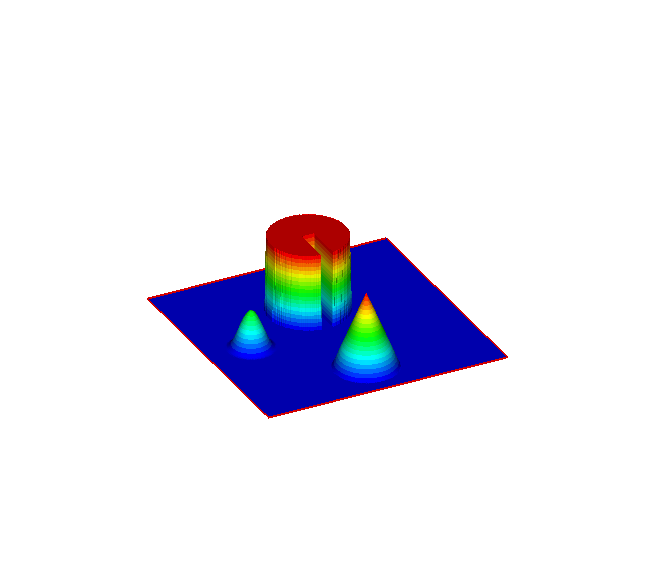
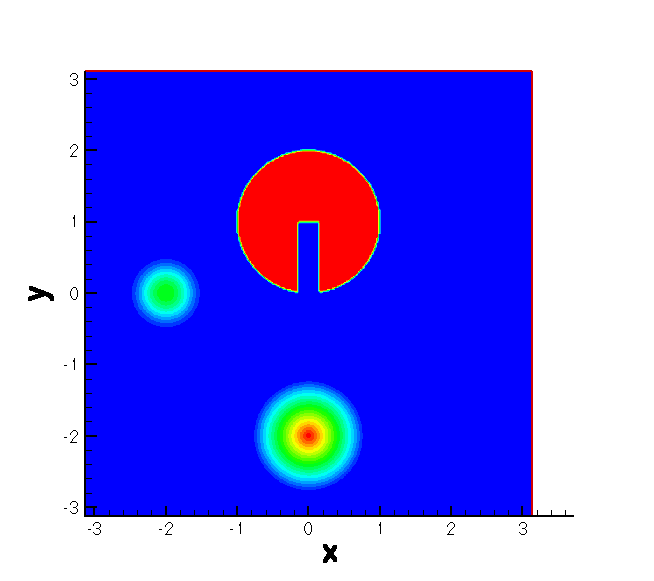
Refer to caption
Refer to caption
Figure 4.4: Initial condition for Example 3.8 and Example 3.9.
Re=100100100 NonMPP MPP
mesh Umax Umin Umax Umin
16×16161616\times 16 0.947915608973 -0.041388485669 0.947719795318 0.000000000000
32×32323232\times 32 0.999789765557 -0.048836983632 0.996173203589 0.000000000000
64×64646464\times 64 1.008171330748 -0.039241271474 0.999999999928 0.000000000000
128×128128128128\times 128 1.002125190412 -0.027962451582 0.999999999920 0.000000000000
256×256256256256\times 256 1.000099518450 -0.012262487330 0.999999999983 0.000000000000
Re=100001000010000 NonMPP MPP
mesh Umax Umin Umax Umin
16×16161616\times 16 0.949247968412 -0.042285048496 0.949049295419 0.000000000000
32×32323232\times 32 1.002247494119 -0.053653247391 0.996943318800 0.000000000000
64×64646464\times 64 1.012845607701 -0.049914946698 0.999999462216 0.000000000000
128×128128128128\times 128 1.009050027036 -0.050526262050 0.999999999977 0.000000000000
256×256256256256\times 256 1.007608558521 -0.058482843302 0.999999999995 0.000000000000
Table 4.10: The maximum and minimum cell averages for rotation problem (4.16) with two different Reynold numbers at T=0.1𝑇0.1T=0.1.
Refer to caption
Refer to caption
Refer to caption
Refer to caption
Figure 4.5: Left: Cutting plots for rotation problem (4.16) for Re=100001000010000 at T=0.1𝑇0.1T=0.1. Right: Zoom-in around the undershooting. Top: cutting along y=5Δy𝑦5Δ𝑦y=5\Delta y for Ny=128subscript𝑁𝑦128N_{y}=128; Bottom: cutting along x=0𝑥0x=0.
Example 4.9.

(Swirling Deformation with Viscosity)

ut+(cos2(x2)sin(y)g(t)u)x+(sin(x)cos2(y2)t(t))u)y=1Re(uxx+uyy),\displaystyle u_{t}+(-\cos^{2}(\frac{x}{2})\sin(y)g(t)u)_{x}+(\sin(x)\cos^{2}(\frac{y}{2})t(t))u)_{y}=\frac{1}{Re}(u_{xx}+u_{yy}), (4.17)

where (x,y)[π,π]2𝑥𝑦superscript𝜋𝜋2(x,y)\in[-\pi,\pi]^{2} and g(t)=cos(πt/T)π𝑔𝑡𝜋𝑡𝑇𝜋g(t)=\cos(\pi t/T)\pi. The initial condition is the same as in Example 4.8 and the boundary conditions are also periodic. Similarly, we also compare the results for different Reynold numbers Re=100100100 and Re=100001000010000. As shown in Table 4.11, the MPP limiter plays the role of eliminating overshooting and undershooting in the numerical solution, especially for problems with larger Reynold number. This can also be observed in Figure 4.6.

Re=100100100 NonMPP MPP
mesh Umax Umin Umax Umin
16×16161616\times 16 0.873440241699 -0.010737472197 0.842184825192 0.000000000000
32×32323232\times 32 0.971822334038 -0.011947680561 0.942384582101 0.000000000000
64×64646464\times 64 0.997563271155 -0.005935366467 0.986960253479 0.000000000000
128×128128128128\times 128 1.000886437426 -0.001258903421 0.998925498573 0.000000000000
256×256256256256\times 256 1.000040508119 -0.000036182185 0.999992956155 0.000000000000
Re=100001000010000 NonMPP MPP
mesh Umax Umin Umax Umin
16×16161616\times 16 0.874953790056 -0.011212471543 0.846813512747 0.000000000000
32×32323232\times 32 0.973964125865 -0.014299538733 0.942368749644 0.000000000000
64×64646464\times 64 1.000873875979 -0.006640227946 0.988604733672 0.000000000000
128×128128128128\times 128 1.002350640870 -0.002755842119 0.999375840770 0.000000000000
256×256256256256\times 256 1.000734372263 -0.000563730690 0.999998986667 0.000000000000
Table 4.11: The maximum and minimum cell averages for swirling deformation problem (4.17) with two different Reynold numbers at T=0.10.10.1.
Refer to caption
Refer to caption
Refer to caption
Refer to caption
Figure 4.6: Left: Cutting plots for swirling deformation problem (4.17) for Re=100001000010000 at T=0.10.10.1. Right: Zoom-in around the undershooting. Top: cutting along y=5Δy𝑦5Δ𝑦y=5\Delta y for Ny=128subscript𝑁𝑦128N_{y}=128; Bottom: cutting along x=0𝑥0x=0.
Example 4.10.

(Vortex Patch) Consider the problem

ωt+(uω)x+(vω)y=1Re(ωxx+ωyy),subscript𝜔𝑡subscript𝑢𝜔𝑥subscript𝑣𝜔𝑦1𝑅𝑒subscript𝜔𝑥𝑥subscript𝜔𝑦𝑦\displaystyle\omega_{t}+(u\omega)_{x}+(v\omega)_{y}=\frac{1}{Re}(\omega_{xx}+\omega_{yy}), (4.18)
Δψ=ω,u,v=ψy,ψx,formulae-sequenceΔ𝜓𝜔𝑢𝑣subscript𝜓𝑦subscript𝜓𝑥\displaystyle\Delta\psi=\omega,\ \langle u,v\rangle=\langle-\psi_{y},\psi_{x}\rangle, (4.19)

with the following initial condition

ω(x,y,0)={1,π2x3π2,π43π4,1,π2x3π2,5π47π4,0,otherwise,𝜔𝑥𝑦0cases1formulae-sequence𝜋2𝑥3𝜋2𝜋43𝜋41formulae-sequence𝜋2𝑥3𝜋25𝜋47𝜋40otherwise\omega(x,y,0)=\begin{cases}-1,\ &\frac{\pi}{2}\leq x\leq\frac{3\pi}{2},\ \frac{\pi}{4}\leq\frac{3\pi}{4},\\ 1,\ \ &\frac{\pi}{2}\leq x\leq\frac{3\pi}{2},\ \frac{5\pi}{4}\leq\frac{7\pi}{4},\\ 0,\ \ &\mbox{otherwise},\end{cases} (4.20)

and periodic boundary condition. The maximum and minimum cell averages of the numerical solution with two Reynold numbers Re=100100100 and Re=100001000010000, obtained by regular FV RK scheme and the scheme with the MPP limiter are compared in Table 4.12, from which we can observe the effectiveness of the MPP limiter in controlling overshooting and undershooting in the numerical solution. The contour plot of the solution is presented in Figure 4.7, which shows that the solution obtained by FV RK scheme with the MPP limiter is comparable to that obtained by regular FV RK scheme.

Re=100100100 NonMPP MPP
mesh Umax Umin Umax Umin
16×16161616\times 16 1.035853749815 -1.035699868274 1.000000000000 -1.000000000000
32×32323232\times 32 1.054573231517 -1.054663726026 1.000000000000 -1.000000000000
64×64646464\times 64 1.044017351861 -1.044000125346 1.000000000000 -1.000000000000
128×128128128128\times 128 1.010637311054 -1.010641150928 1.000000000000 -1.000000000000
256×256256256256\times 256 1.000000232315 -1.000000231632 1.000000000000 -1.000000000000
Re=100001000010000 NonMPP MPP
mesh Umax Umin Umax Umin
16×16161616\times 16 1.036117022938 -1.035951331163 1.000000000000 -1.000000000000
32×32323232\times 32 1.060652217270 -1.060764279809 1.000000000000 -1.000000000000
64×64646464\times 64 1.086490500643 -1.086296444198 1.000000000000 -1.000000000000
128×128128128128\times 128 1.127323843780 -1.127407543973 1.000000000000 -1.000000000000
256×256256256256\times 256 1.129384376147 -1.129395445889 1.000000000000 -1.000000000000
Table 4.12: The maximum and minimum cell averages for vortex patch problem (4.18) at time T=0.10.10.1 with Re=100100100 and Re=100001000010000.
Refer to caption

, Refer to caption
Refer to caption, Refer to caption

Figure 4.7: Contours of the numerical solution for vortex patch problem (4.18) with Re=100100100 (top) and Re=100001000010000 (bottom) at time T=5𝑇5T=5. The contours on the left are for the NonMPP scheme and those on the right are for the MPP scheme. 30 equally spaced contour lines within the range [1.1,1.1]1.11.1[-1.1,1.1] are plotted.

5 Conclusion

In this paper, we have successfully generalized the MPP flux limiters to the high order FV RK WENO schemes solving convection-dominated problems. For a special case, f(u)>0superscript𝑓𝑢0f^{\prime}(u)>0 or f(u)<0superscript𝑓𝑢0f^{\prime}(u)<0, we provide a complete analysis that the original high order FV RK WENO scheme coupled with the MPP flux limiters maintains high order accuracy and MPP property when Godunov type flux is used as the first order flux, toward which the high order numerical flux is limited. For a general setting, we rely on the Taylor expansion around extrema to prove that the FV RK schemes with MPP flux limiters preserve up to third order accuracy without addition CFL constraint. Establishing analysis for accuracy preservation under suitable constraints in a general setting will be part of our future work.

References

  • [1] B. Cockburn, C. Johnson, C.-W. Shu, and E. Tadmor, Advanced numerical approximation of nonlinear hyperbolic equations, Springer New York, 1998.
  • [2] I. Faragó and R. Horváth, Discrete maximum principle and adequate discretizations of linear parabolic problems, SIAM Journal on Scientific Computing, 28 (2006), pp. 2313–2336.
  • [3] I. Faragó, R. Horváth, and S. Korotov, Discrete maximum principle for linear parabolic problems solved on hybrid meshes, Applied Numerical Mathematics, 53 (2005), pp. 249–264.
  • [4] I. Faragó and J. Karátson, Discrete maximum principle for nonlinear parabolic PDE systems, IMA Journal of Numerical Analysis, (2012).
  • [5] H. Fujii, Some remarks on finite element analysis of time-dependent field problems, Theory and Practice in Finite Element Structural Analysis, (1973), pp. 91–106.
  • [6] S. Gottlieb, D. Ketcheson, and C.-W. Shu, High order strong stability preserving time discretizations, Journal of Scientific Computing, 38 (2009), pp. 251–289.
  • [7] A. Harten, High resolution schemes for hyperbolic conservation laws, Journal of Computational Physics, 49 (1983), pp. 357–393.
  • [8] X. Y. Hu, N. A. Adams, and C.-W. Shu, Positivity-preserving method for high-order conservative schemes solving compressible Euler equations, Journal of Computational Physics, 242 (2013), pp. 169–180.
  • [9] Y. Jiang and Z. Xu, Parametrized maximum principle preserving limiter for finite difference WENO schemes solving convection-dominated diffusion equations, SIAM Journal on Scientific Computing, 35 (2013), pp. A2524–A2553.
  • [10] C. Liang and Z. Xu, Parametrized maximum principle preserving flux limiters for high order schemes solving multi-dimensional scalar hyperbolic conservation laws, Journal of Scientific Computing, 58 (2014), pp. 41–60.
  • [11] B. Perthame and C.-W. Shu, On positivity preserving finite volume schemes for Euler equations, Numerische Mathematik, 73 (1996), pp. 119–130.
  • [12] T. Xiong, J.-M. Qiu, and Z. Xu, A parametrized maximum principle preserving flux limiter for finite difference RK-WENO schemes with applications in incompressible flows , Journal of Computational Physics, 252 (2013), pp. 310–331.
  • [13]  , Parametrized positivity preserving flux limiters for the high order finite difference WENO scheme solving compressible Euler equations, (submitted).
  • [14]  , Semi-Lagrangian finite difference WENO scheme with parametrized MPP flux limiters for the Vlasov equation, (submitted).
  • [15] Z. Xu, Parametrized maximum principle preserving flux limiters for high order scheme solving hyperbolic conservation laws: one-dimensional scalar problem, Mathematics of Computation, (in press).
  • [16] X. Zhang, Y. Liu, and C.-W. Shu, Maximum-principle-satisfying high order finite volume weighted essentially nonoscillatory schemes for convection-diffusion equations, SIAM Journal on Scientific Computing, 34 (2012), pp. A627–A658.
  • [17] X. Zhang and C.-W. Shu, On maximum-principle-satisfying high order schemes for scalar conservation laws, Journal of Computational Physics, 229 (2010), pp. 3091–3120.
  • [18]  , On positivity-preserving high order discontinuous Galerkin schemes for compressible Euler equations on rectangular meshes, Journal of Computational Physics, 229 (2010), pp. 8918–8934.
  • [19] Y. Zhang, X. Zhang, and C.-W. Shu, Maximum-principle-satisfying second order discontinuous Galerkin schemes for convection-diffusion equations on triangular meshes, Journal of Computational Physics, 234 (2012), pp. 295–316.