The charged McVittie spacetime
Abstract
The two-parameter charged McVittie solution of the Einstein equations is revisited and its apparent horizons are discussed and located numerically (for the extremal case, analytically). According to the parameter values, this spacetime can be interpreted as a black hole, or a spacelike naked singularity, in a spatially homogeneous and isotropic universe.
pacs:
98.80.-k, 04.50.+hI Introduction
Analytical solutions of general relativity and of alternative theories of gravity which represent inhomogeneous cosmologies have been the subject of much recent interest. In the context of general relativity, spherically symmetric solutions of this kind are used to explore alternatives to dark energy in explaining the current acceleration of the cosmic expansion (see Ref. voids for a review), to study the effect of the cosmic dynamics on local systems CarreraGiulini , to study the spatial variation of fundamental constants Barrow , and to explore the thermodynamics of time-dependent horizons SaidaHaradaMaeda ; myPRD ; Majhi ; myreview . Solutions representing time-varying black holes are of interest in themselves and the first spacetime of this kind is the 1933 McVittie solution of the Einstein equations constructed to study the effect of the cosmic dynamics on a local system McVittie . It describes a central inhomogeneity in a Friedmann-Lemâitre-Robertson-Walker (FLRW) “background”. Over the years, the McVittie solution has been the subject of many studies oldMcVittie but it is not yet completely understood, as testified by the proliferation of recent works CarreraGiulini10 ; Klebanetal ; LakeAbdelqader ; Anderson ; Roshinaetal ; AndresRoshina ; SilvaFontaniniGuariento . Most recently, it has been shown that the McVittie metric cannot be generated as a scalar field solution unless non-canonical scalars, introduced in the literature as forms of exotic dark energy, are employed — this is the case of the cuscuton theory, a special case of Horava-Lifschitz theory, of which the McVittie metric is a solution cuscuton .
A charged version of the original McVittie metric was found by Gao and Zhang GaoZhang , who also generalized it to higher dimensions McVittieHigherD , and was discussed very briefly in McClureDyerCQG ; McClureThesis . Here we want to refine the rather cursory analysis of this metric presented in these references and, in particular, locate its apparent horizons (when present) and study their dynamics.
Conformal diagrams of the McVittie spacetime for various backgrounds were obtained in LakeAbdelqader ; SilvaFontaniniGuariento and we expect them to be qualitatively similar in the charged case; however we do not get into such level of detail here. As an application of the charged McVittie spacetime, we mention that it was used111The analysis of Ref. bhareas is flawed by a typographical error present in the metric of GaoZhang but, as we shall see, the qualitative behaviour of the apparent horizons for does not change and the argument of Ref. bhareas still stands. to disprove the universality of certain quantization laws for quantities constructed with the areas of black hole apparent horizons and inspired by string theories bhareas .
II The charged McVittie spacetime and its apparent horizons
For simplicity we restrict ourselves to a spatially flat FLRW “background” (we use quotation marks because, due to the non-linearity of the Einstein equations, it is in general impossible to split a metric into a background and a deviation from it in a covariant way). The spherically symmetric, non-stationary, charged McVittie line element and the only nonvanishing component of the Maxwell tensor are222Our notations differ slightly from those of Ref. GaoZhang . Beware of a typographical error in the numerator of in GaoZhang , which was corrected in Refs. McVittieHigherD ; McClureDyerCQG ; McClureThesis .
where is the isotropic radius, is the line element on the unit 2-sphere, the constants and are a mass and an electric charge parameter, respectively, and is the scale factor of the “background” FLRW universe. If , the line element (LABEL:QMcVlineelement) reduces to the Reissner-Nordström one in isotropic coordinates while, for large values of , it reduces to the spatially flat FLRW metric. If , the metric becomes an exact spatially flat FLRW one.
The inspection of eq. (LABEL:QMcVlineelement) provides immediately the areal radius
| (3) | |||||
and it is for . Assuming the range of parameters , the function (and consequently also the area of 2-spheres of symmetry) decreases from in the range , has an absolute minimum at , and increases again to plus infinity for , which shows clearly that the isotropic radius corresponds to a double covering of the spacetime region . (This fact is well known for the Schwarzschild spacetime Buchdhal , which is contained in the metric (LABEL:QMcVlineelement) as the special case .)
In the case , the areal radius is instead a monotonically increasing function of and the physically meaningful region corresponds to .
The relation between areal radius and isotropic radius can be inverted, which will be useful in the following to study the horizons of the charged McVittie spacetime. This inversion gives the quadratic equation
| (4) |
with the positive root satisfying the relation
| (5) |
The Ricci scalar is found to be
| (6) |
The non-zero components of the Einstein tensor are333The expression of the Einstein tensor in Refs. McClureDyerCQG and McClureThesis differs from ours in that, there, a scale factor term is missing in the combination in the denominators.
| (7) | ||||
| (8) | ||||
| (9) |
is the Hubble parameter of the FLRW “background” and an overdot denotes differentiation with respect to the comoving time . The vanishing of implies that there is no accretion (which, to respect the symmetry, could only be radial) of cosmic fluid onto the central object.
For eq. (6) reduces to the well known Ricci scalar of the spatially flat FLRW universe . For it reduces to zero, which is the Ricci scalar of the Reissner-Nordström spacetime (the only source of matter is then the Maxwell field with traceless energy-momentum tensor). If there is a singularity where , or
| (10) |
corresponding to the areal radius
| (11) |
which is precisely the location of the outer event horizon of Reissner-Nordström spacetime (the limit).
For the extremal case the metric becomes
| (12) |
and the singularity occurs at which corresponds to the areal radius , again coinciding with the location of the outer event horizon of the Reissner-Nordström limit, in this case the single event horizon of the extremal Reissner-Nordström black hole.
This new spherical singularity is not present if . In this case, however, the scalar invariant of the Maxwell tensor
| (13) |
diverges at
| (14) |
corresponding to due to the divergence of the radial electric field, which is the only non-zero component of the Maxwell tensor. Of course, the Big Bang singularity is always present at . The singularity (11) divides the spacetime into two disconnected manifolds, as in the McVittie case Nolan ; oldMcVittie .
The spacetime singularity (11) (for ) is spacelike. In fact, this singularity corresponds to , where
| (15) |
we have
| (16) | |||||
In the limit in which from above, this expression tends to , therefore the norm of the normal to the surfaces const. in this limit is negative, hence this surface and its limit are spacelike.
The black hole nature of the charged McVittie spacetime is assessed by examining its horizons. Since the metric is dynamical, the relevant concept of horizon is not the null and teleological event horizon, which requires the knowledge of the entire spacetime manifold to future null infinity. Apparent and trapping horizons, instead, are more appropriate and useful concepts to describe dynamical situations Alexreview ; Ivanreview ; AshtekarKrishnan ; myreview , and we will study the apparent horizons, which are located by the equation (e.g., NielsenVisser ; AbreuVisser ; myreview ), where is the areal radius. After straightforward manipulations, this equation becomes
| (17) | |||||
Excluding the singularity (11), the roots of (17) are the roots of the equation
| (18) |
It is useful to express the location of the apparent horizons in terms of the physical (areal) radius, obtaining
| (19) |
where is given by eq. (5). Equation (19) can be manipulated without further approximation to the quartic polynomial in
| (20) |
Note that this polynomial is general and applies independently of the relation of to . For large values of this equation reduces to , the value of the radius of the apparent horizon of the spatially flat FLRW “background”, which makes us expect a cosmological horizon to be present. In any regime in which (for example in power law backgrounds with and hence as ), eq. (19) reduces to its asymptotic form
| (21) |
so that, in this limit
| (22) |
implying that at late times in any region of a background for which (for example late times in a power law background) a black hole apparent horizon asymptotes to the singularity (11) from above. Note that the smaller root always lies inside the spherical singularity and that these two roots exactly coincide with the locations of the two event horizons of Reissner-Nordström. Hence we see that the limit reproduces the horizon structure of the static Reissner-Nordström spacetime.444Albeit with the addition of the spherical singularity not present in Reissner-Nordström. This spherical singularity is present even when and independently of the time dependence , as long as it is not exactly constant. The authors are currently investigating further this curious feature of the charged and uncharged McVitte spacetime.
II.1 Dust-dominated background
Let us restrict now, for the sake of example, to a dust-dominated background with and . Consider the case . Then eq. (20) can be solved explicitly at different times giving the location of the apparent horizons. These are plotted versus comoving time in Fig. 1 for a choice of parameters. The phenomenology of these apparent horizons is similar to that found for the uncharged McVittie solution Nolan ; Klebanetal ; LakeAbdelqader ; AndresRoshina .
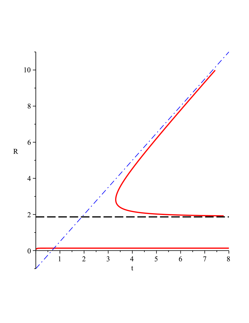
Initially (near the Big Bang ), there are no apparent horizons in the connected outer region beyond the spherical singularity; at a critical time a cosmological and a black hole apparent horizon appear. The black hole apparent horizon shrinks asymptoting to the singularity, while the cosmological apparent horizon expands forever. This phenomenology is interpreted in AndresRoshina for by noting that at early times the size of the black hole horizon exceeds that of the cosmological horizon and such a large black hole cannot be accomodated in a small universe. (This situation is similar to that of the Schwarzschild-de Sitter black hole, which is a special case of the McVittie metric AndresRoshina .) Later on, the cosmological horizon becomes larger than the black hole apparent horizon, which now fits below the cosmological horizon AndresRoshina .
Note that the innermost apparent horizon, which asymptotes to the location of the inner unstable Cauchy horizon of Reissner-Nordström geometry, is located in the inner disconnected region, separated from the exterior geometry by the singularity (11), converging to at the Big Bang.
II.2 Universe undergoing finite expansion
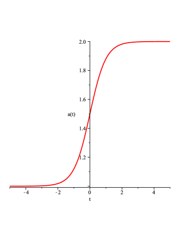
As a toy model to further investigate the interesting apparent horizon structures, let us consider a universe undergoing a finite expansion from an initially quasi-static regime to a final quasi-static regime with scale factor
| (23) |
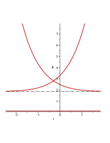
Shown in Fig. 2 is the scale factor (23) for the choice , , and representing a universe which expands by a factor of 2 from to . We consider only the case for the rest of this subsection and also fix the values and for illustration.
The horizon phenomenology in this case depends on the time scale of expansion with horizon mergers and horizon joinings possible. In Fig. 3 we plot the roots of the polynomial (20) over time for a ‘fast’ expansion () where the cosmological horizon shrinks from to eventually merge with the expanding black hole horizon leaving a naked singularity for a period followed by the birth again of two horizons which separate, the cosmological one out to and the black hole horizon asymptoting to the spherical singularity at .
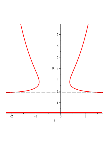
Note that the horizon structure is not symmetric about since it is the asymmetric function which enters the quartic polynomial defining the horizon locations. In Fig. 4 we plot the location of the apparent horizons over time for a “slow” expansion () where the cosmological horizon does not shrink enough to subsume the black hole horizon. In this slow case, the spherical singularity is always hidden behind an apparent horizon for asymptotic observers far from the inhomogeneity.
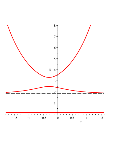
Interestingly, the curious limiting case in which the cosmological and black hole horizons meet at a point, appearing to intersect, can be solved for exactly, occurring when the Hubble parameter attains a critical value at its maximum leaving a single apparent horizon at in the exterior region, where
| (24) | ||||
| (25) |
Such a scenario is shown in Fig. 5, where we see the “crossing” of the horizons at a single time.
II.3 The extremal case
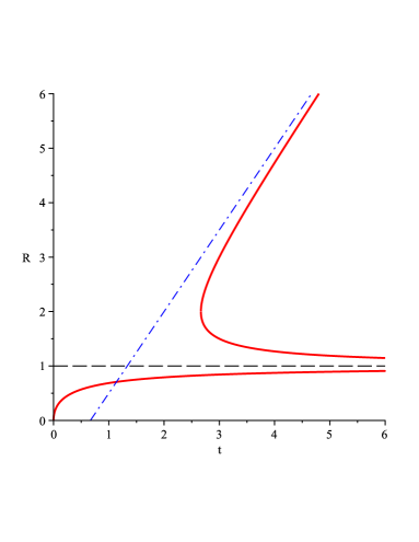
In the extremal case with the quartic relation (20) is exactly solvable, with solutions
| (26) |
The extremal case is interesting in the sense that an explicit analytical expression like (26) for the apparent horizon radii is rare to find in investigations of time-evolving black holes myreview . One of these roots is always negative and hence is discarded
| (27) |
The smallest positive root given by
| (28) |
is always present while the other two
| (29) |
can merge (become complex) or appear simultaneously (become real) depending on the evolution of . Interestingly, for the dust-dominated background as and we see that and in fact converge to the same radius . This common limit radius is precisely where the single event horizon of extremal Reissner-Nordström sits, nicely showing that we recover the phenomenology of the static charged spacetime in the appropriate limit. This horizon behaviour is shown in Fig. 6.
II.4 The supercritical case
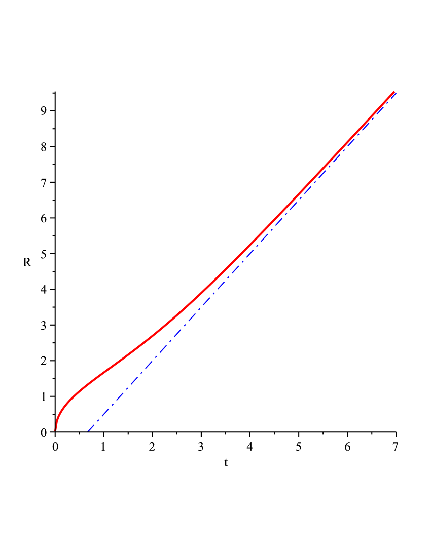
In the case we expect a naked singularity, based on the limit of constant which reproduces the Reissner-Nordström spacetime. The cosmological horizon is still present, as expected from the previous considerations. In fact, numerical plots for this situation provide a single (cosmological) apparent horizon, as shown in Fig. 7.
III Discussion
In the parameter range explored we find only a cosmological apparent horizon and one black hole apparent horizon, while in the Reissner-Nordström black hole (to which the metric reduces if ) it is well known that also an inner black hole (apparent) horizon is present. This fact begs the question of why, in the charged McVittie spacetime which generalizes the Reissner-Nordström metric, we do not see an inner black hole horizon in addition to the cosmological horizon. The inner black hole horizon of the Reissner-Nordström black hole is unstable with respect to linear perturbations and the effect of the cosmological “background” on the central inhomogeneity is akin to a non-linear (or exact) “large perturbation”, therefore, the absence of an inner black hole horizon is not too surprising in this regard.555However, this “perturbation” is not “small”, in the sense that it corresponds to an infinite amount of mass-energy added to the Reissner-Nordström spacetime, even in the case of arbitrarily small density of the FLRW “background”. Moreover, the density diverges at the spherical singularity. We expect such an horizon to be absent in any exact solution of the Einstein equations describing a Reissner-Nordström-like black hole interacting with a non-trivial environment.
Acknowledgements.
This work is supported by Bishop’s University and by the Natural Sciences and Engineering Research Council of Canada.References
- (1) K. Boleiko, M.-N. Célérier and A. Krasinski, Class. Quantum Grav. 28 164002 (2011).
- (2) M. Carrera and D. Giulini, Rev. Mod. Phys. 82, 169 (2010).
- (3) J.D. Barrow and C. O’Toole, Mon. Not. R. Astron. Soc. 322, 585 (2001); N. Sakai and J.D. Barrow, Class. Quantum Grav. 18, 4717 (2001); T. Clifton, D.F. Mota, and J.D. Barrow, Mon. Astron. Soc. 358, 601 (2005); V. Faraoni, V. Vitagliano, T.P. Sotiriou, and S. Liberati, Phys. Rev. D 86, 064040 (2012).
- (4) H. Saida, T. Harada, and H. Maeda, Class. Quantum Grav. 24, 4711 (2007).
- (5) V. Faraoni, Phys. Rev. D 76, 104042 (2007).
- (6) B.R. Majhi, arXiv:1403.4058.
- (7) V. Faraoni, Galaxies 1, 114 (2013).
- (8) G.C. McVittie, Mon. Not. R. Astron. Soc. 93, 325 (1933).
- (9) A. Krasinski, Inhomogeneous Cosmological Models (Cambridge University Press, Cambridge, UK, 1997); M. Ferraris, M. Francaviglia, and A. Spallicci, Nuovo Cimento 111B, 1031 (1996); B.C. Nolan, J. Math. Phys. 34, 178 (1993); Phys. Rev. D 58, 064006 (1998); Class. Quantum Grav. 16, 1227 (1999); V. Faraoni and A. Jacques, Phys. Rev. D 76, 063510 (2007); Z.-H. Li and A. Wang, Mod. Phys. Lett. A 22, 1663 (2007); V. Faraoni, C. Gao, X. Chen, and Y.-G. Shen, Phys. Lett. B 671, 7 (2009).
- (10) M. Carrera and D. Giulini, Phys. Rev. D 81, 043521 (2010).
- (11) N. Kaloper, M. Kleban, and D. Martin, Phys. Rev. D 81, 104044 (2010).
- (12) K. Lake and M. Abdelqader, Phys. Rev. D 84, 044045 (2011); P. Landry, M. Abdelqader, and K. Lake, Phys. Rev. D 86, 084002 (2012).
- (13) M. Anderson, J. Phys. Conf. Ser. 283, 012001 (2011).
- (14) R. Nandra, A.N. Lasenby, and M.P. Hobson, Mon. Not. R. Astron. Soc. 422, 2931 (2012); 422, 2945 (2012).
- (15) V. Faraoni, A.F. Zambrano Moreno, and R. Nandra, Phys. Rev. D 85, 083526 (2012).
- (16) A. Da Silva, M. Fontanini, and D.C. Guariento, Phys. Rev. D 87, 064030 (2013); M. Le Delliou, J.P. Mimoso, F.C. Mena, M. Fontanini, D.C. Guariento, and E. Abdalla, Phys. Rev. D 88, 027301 (2013).
- (17) E. Abdalla, N. Afshordi, M. Fontanini, D.C. Guariento, and E. Papantonopoulos, arXiv:1312.3682.
- (18) C.J. Gao and S.N. Zhang, Phys. Lett. B 595, 28 (2004).
- (19) C.J. Gao and S.N Zhang, Gen. Rel. Gravit. 38, 23 (2006).
- (20) M.L. McClure and C.C. Dyer, Class. Quantum Grav. 23, 1971 (2006).
- (21) M.L. McClure, Cosmological Black Holes as Models of Cosmological Inhomogeneities, PhD thesis, University of Toronto, 2006.
- (22) V. Faraoni and A.F. Zambrano Moreno, Phys. Rev. D 88, 044011 (2013).
- (23) H. Weyl, Ann. Phys. (Leipzig) 54, 117 (1917); H.A. Buchdhal, Int. J. Theor. Phys. 24, 731 (1985).
- (24) A.B. Nielsen, Gen. Rel. Gravit. 41, 1539 (2009).
- (25) I. Booth, Can. J. Phys. 83, 1073 (2005).
- (26) A. Ashtekar and B. Krishnan, Living Rev. Relativ. 7, 10 (2004).
- (27) A.B. Nielsen and M. Visser, Class. Quantum Grav. 23, 4637 (2006).
- (28) G. Abreu and M. Visser, Phys. Rev. D 82, 044027 (2010).
- (29) B.C. Nolan, Phys. Rev. D 58, 064006 (1998); Class. Quantum Grav. 16, 1227 (1999).
