Optimal Rendezvous Strategies for Different Environments in Cognitive Radio Networks

Abstract

In Cognitive Radio Networks (CRNs), the secondary users (SUs) are allowed to access the licensed channels opportunistically. A fundamental and essential operation for SUs is to establish communication through choosing a common channel at the same time slot, which is referred to as rendezvous problem. In this paper, we study strategies to achieve fast rendezvous for two secondary users.

The channel availability for secondary nodes is subject to temporal and spatial variation. Moreover, in a distributed system, one user is oblivious of the other user’s channel status. Therefore, a fast rendezvous is not trivial. Recently, a number of rendezvous strategies have been proposed for different system settings, but rarely have they taken the temporal variation of the channels into account. In this work, we first derive a time-adaptive strategy with optimal expected time-to-rendezvous (TTR) for synchronous systems in stable environments, where channel availability is assumed to be static over time. Next, in dynamic environments, which better represent temporally dynamic channel availability in CRNs, we first derive optimal strategies for two special cases, and then prove that our strategy is still asymptotically optimal in general dynamic cases.

Numerous simulations are conducted to demonstrate the performance of our strategies, and validate the theoretical analysis. The impacts of different parameters on the TTR are also investigated, such as the number of channels, the channel open possibilities, the extent of the environment being dynamic, and the existence of an intruder.

1 Introduction

1.1 Background

The number of wireless devices has skyrocketed over the last decade, which exasperates the scarcity of spectral resources. The reality is that most wireless spectrum bands have been allocated by regulatory agencies to licensed users, which however are severely under-utilized. It is reported that the utilization of licensed spectrum varies from $15\%$ to $85\%$ [1], and only $5\%$ of the spectrum from $30$ Mhz to $30$ GHz is used in the US [7]. Recently some regulators have issued permissions for unlicensed devices to use parts of the licensed spectrum under restrictions. Cognitive Radio (CR) realizes the unlicensed devices (called secondary users) to utilize the temporarily unused licensed spectrums without interfering with the licensed devices (called primary users). Therefore, CR is a promising technology to alleviate the spectrum shortage problem in wireless communication, and Cognitive Radio Network (CRN) is considered the next generation of communication networks.

In a CRN, through spectrum sensing [18], each secondary user (SU) has the ability to detect current open (or available) channels at its site, i.e., channels that are not occupied by the primary users (PUs). Due to dynamic come and go of PUs, the available channels to SUs have the following important characteristics: 1) Spatial Variation: SUs at different locations may have different available channels; and 2)Temporal Variation: the available channels of a SU may change over time.

Spectrum assignment is to allocate available channels to SUs to improve network performance, such as connectivity, spectrum utilization, network throughput and fairness [11, 13, 16, 20, 21]. Spectrum assignment is one of the most challenging problems in CRNs. One fundamental action in spectrum assignment is referred to as the rendezvous problem of which the simplest form can be stated as:

For two secondary users, Alice and Bob, how do they establish a connection through choosing a common channel at the same time slot?

We call the approach they adopt for choosing a channel at each round as a rendezvous strategy. A strategy attaining a fast time-to-rendezvous (TTR) is not trivial due to the following facts: 1) the local available channels for Alice and Bob are asymmetric; 2) in a distributed system, one SU only knows his/her local channel status but not the other’s; 3) the local channel availability may change during the rendezvous; and 4) in asynchronous systems, rendezvous is even more complicated as one does not know the time of the other SU or how many tries the other SU has made.

1.2 Related Work

1.2.1 Basic Rendezvous Problem and its Variants

In the basic form of the Rendezvous problem (also called the telephone coordination game [4]), two players are placed in two separated rooms each with $n$ telephone lines. There is a one-to-one matching between the lines in two rooms, and players can only use matched lines to contact each other; the matching is not known to either of the players. In every round each player can select a line in his room and see whether it is connected with the line chosen by another player. The goal is to design a strategy for the players to get connected while minimizing the number of trial rounds.

It is not hard to see that the optimal strategy takes $n/2$ rounds in expectation, which is achievable by letting the first player choose a random line and keep using it, and letting the second player try the lines one by one in a random order. However, this strategy only works when the players can correctly determine who is the first player, which may not be possible in a given application. Thus, a player-independent strategy is desired. Anderson and Weber [5] presented such a strategy using at most $0.829n$ rounds in expectation, where each player will repeat either to keep on choosing one line or randomly choosing a line different from his last choice with some probabilities. There are many other well-studied variants of the Rendezvous problem; see, e.g., [2, 3] and the references therein. Also, some researcher considered jammers in rendezvous, such as the node discovery in (conventional) multiple-channel wireless communications [14].

1.2.2 Rendezvous in CRNs

In contrast to the basic version, rendezvous in CRNs happens in an asymmetric dynamic scenario, where each user may have different and time-variant sets of available channels. There have been a number of rendezvous strategies proposed for CRNs. One group of these strategies makes use of a dedicated channel, called a Common Control Channel (CCC), to exchange information between users for rendezvous (e.g.,  [8, 10, 15, 22]). However, assuming a CCC might not be practical as the channel could be occupied by some PUs, and it also introduces an easy attack point. Blind rendezvous without any centralized controller or a dedicated CCC is therefore preferred (in this paper, unless specified otherwise, rendezvous stands for this blind case). A main group of these rendezvous strategies adopts the channel-hopping (CH) technique, where SUs hop among their available channels based on a hopping sequence to achieve rendezvous (e.g., [9, 12, 19]). Quorum Systems are also frequently adopted for rendezvous in CRNs(e.g., [17]). Besides, in paper  [6], Azar et. al. proposed an strategy using geometric distribution for asynchronous systems, and proved it to be optimal when there are a large number of channels. Essential details of their strategy will be covered in Section 3.1. Although most of the above work have considered the spatial variation of the channels, i.e., users in different locations may have different sets of available channels, they are limited to stable (channel) environments where the channel availabilities are static over time. Not many of them take the temporal variation of channels into account. In this work, we will study both the stable and the dynamic environment in asynchronous and synchronous systems. We hope this work may inspire further research on the dynamic version of the rendezvous problem.

1.3 Our Results

In this paper, we investigate the rendezvous problem for two SUs and derive optimal strategies for different system settings. For the sake of theoretical analysis, we assume each channel of Alice and Bob has an available probability of $p_{a}$ and $p_{b}$ respectively, and denote the total number of channels as $n$. Our results can be summarized as follows:

• For a synchronous stable environment, we derive a time-adaptive strategy that guarantees successful rendezvous at the first common channel, say channel $m$, within at most $m$ rounds. The expected TTR of our strategy is $\frac{2-\max(p_{a},p_{b})}{\min(p_{a},p_{b})}$ when $n\rightarrow+\infty$, which is a 2-approximation to the optimal.

• Our main effort is devoted to the dynamic environments which better reflect the nature of temporal variation of channel availability in CRNs. We first define two special cases, the semi-stable and the independent dynamic cases (refer to Section 4). For the synchronous semi-stable case, we derive an optimal strategy based on the one used in the synchronous stable environment. For the independent dynamic environment, we derive a simple stationary strategy and prove that it is exactly optimal no matter whether there is a common clock or not. When $n\rightarrow+\infty$, its expected TTR is $\frac{1}{p_{a}}+\frac{1}{p_{b}}-1$. Then, we model the channel availability in the general dynamic environment as a Markov process. When neither of the environments of two SUs is stable nor semi-stable, we prove the expected TTR of our strategy is $O\left(\ln\left(\frac{1}{\min(p_{a},p_{b})}\right)\cdot\left(\frac{1}{p_{a}}+\frac{1}{p_{b}}-1\right)\right)$, which is asymptotically optimal.

• Based on simulation, we validate the above theoretical analysis and demonstrate the efficiency of our strategies when there are a small number of channels. Besides, we reveal the impacts of different parameters on the TTR, such as the number of channels, the channel open possibilities, the extent to which the environment being dynamic, and the existence of an intruder.

Paper Organization: In Section 2, we formally define our model and problems studied in this paper. We investigate the rendezvous problem in stable environments in Section 3. The different cases in dynamic environments are studied in Sections 4. Section 5 gives the simulation results and discussions. The whole paper is concluded in Section 6 with possible future works.

2 Problem Definition

We consider a pair of secondary nodes, called Alice and Bob, which need to establish a connection. There are totally $n$ channels with ID’s from $1$ to $n$. A binary vector $A^{t}=\{A_{1}^{t},A_{2}^{t},\ldots,A_{n}^{t}\}$ indicates whether a channel is open for Alice at time $t$, e.g., if channel $i$ is open at time $t$, $A_{i}^{t}=1$; otherwise, $A_{i}^{t}=0$. Vector $B^{t}$ is similarly defined for Bob. Through spectrum sensing, both Alice and Bob can know their local available channels. However, as in a distributed system, Alice and Bob are oblivious of $B^{t}$ and $A^{t}$, respectively. In addition, there is no information (i.e., the node IDs) to break the symmetry of the two nodes.

We investigate both synchronous and asynchronous distributed systems in stable and dynamic environments. In a synchronous system, Alice and Bob will have a common clock, whereas in an asynchronous system, they do not know each other’s clock. As mentioned before, in a stable environment, the channel availability will be static over time, while in a dynamic environment, the channel status may change over time. We assume at least one common channel exists in the channel environment, or otherwise the rendezvous can never happen. Within a round (time slot), each node will try to achieve rendezvous once using a strategy which is stationary or adaptive over the rounds.

Table 1: Definitions of the symbols

Symbol	Definition
$n$	the total number of channels
$A_{i}^{t}$ or $B_{i}^{t}$	availability of channel $i$ for Alice or Bob at time $t$
$\mathcal{S}_{a}$ or $\mathcal{S}_{b}$	the strategy of Alice or Bob
$\mathcal{S}_{a}^{t}(i)$ or $\mathcal{S}_{b}^{t}(i)$	the probability that Alice or Bob chooses channel $i$ at time slot $t$
$\phi_{t}$	the flag indicating whether a rendezvous is achieved successfully at time $t$
$TTR$	the time-to-rendezvous

In CRNs, one node might wake up and start trying rendezvous earlier than the other. These tries will definitely fail. Thus, we count the time-to-rendezvous (TTR) from the starting point when both Alice and Bob have waken up. Based on the symbols in Table 1, the possibility for a successful rendezvous at $t$ is $Pr[\phi_{t}=1|\{A_{i}^{t}\},\{B_{i}^{t}\}]=\sum^{n}_{i=1}A_{i}^{t}B_{i}^{t}\mathcal{S}_{a}^{t}(i)\mathcal{S}_{b}^{t}(i).$ The TTR is the first instant when Alice and Bob choose a common channel simultaneously: $TTR=\min\{t:\phi_{t}=1\}$. Our goal is to derive strategies for Alice and Bob that minimize $E[TTR]$, the expectation of TTR.

For convenience of analysis, at any round we assume each channel $i$ of Alice has a probability of $p_{a}$ to be open ($0<p_{a}\leq 1$) independently. That is to say, for Alice, in the dynamic environment, without the knowledge of the channel status in previous slots, $Pr[A^{t}_{i}=1]=p_{a}$, $\forall t\geq 1$; in the stable environment, each channel will open with probability of $p_{a}$ at the first time slot and never change status subsequently. $p_{b}$ is similarly defined for Bob.

3 Stable Environment

3.1 Strategy for Asynchronous Systems

In an asynchronous system, as there is no common clock, neither of Alice and Bob know the time of the other player nor how many time slots the other player has tried for rendezvous. Therefore, a strategy that is adaptive to time is meaningless, and stationary strategies are required. In [6], the authors proposed a stationary strategy based on geometric distributions shown as Strategy A in Appendix A. Its expected TTR is proved to be $O(\frac{1}{p_{a}p_{b}})$ when $n\rightarrow+\infty$. In addition, it is proved that the strategy is essentially optimal as the TTR of any stationary strategy is $\Omega(\frac{1}{p_{a}p_{b}})$. However, a main weakness of Strategy A is that Alice (Bob) has to have the knowledge of $p_{b}$ ($p_{a}$), which might be not feasible in practice.

Next, we will extend their work and present our simple optimal strategy in synchronous stable environments which guarantees a fast rendezvous and is applicable for finite channels.

3.2 Strategy for Synchronous Systems

In a synchronous system, although one user is oblivious of the other user’s channel status, he/she is aware of the time of the other user. Therefore, we can derive non-stationary strategies that are adaptive to time:

Strategy B:
In the $i$-th round ($i\geq 1$),
$\mathcal{S}_{a}$: Alice chooses her first local open channel from channel $i$ to channel $n$; that is, she chooses channel $a^{*}=\min\{a~{}|~{}A_{a}^{i}=1;i\leq a\leq n\}$.
$\mathcal{S}_{b}$: Bob chooses his first local open channel from channel $i$ to channel $n$; that is, he chooses channel $b^{*}=\min\{b~{}|~{}B_{b}^{i}=1;i\leq b\leq n\}$.

Strategy B is actually a novel waiting-to-meeting scheme: the one who reaches the first common open channel will stick to it until the other reaches that same channel when they achieve rendezvous. Therefore, we have this theorem:

Theorem 1.

Suppose the first common open channel of Alice and Bob is channel $m$. With Strategy B, they will definitely achieve rendezvous on $m$ with no more than $m$ rounds in synchronous stable environments.

Next, we prove the optimality of our strategy.

Theorem 2.

In the synchronous stable environment, when $n\rightarrow+\infty$, the expected TTR of Strategy B satisfies $E[TTR]\leq\frac{2-\max(p_{a},p_{b})}{\min(p_{a},p_{b})},$ which is a 2-approximation to the optimal.

Proof.

At $i$-th round, if Alice chooses channel $i+k$ where $0\leq k\leq n-i$, it means that channels $i,i+1,\ldots,i+k-1$ are all closed and that channel $i+k$ is open. In addition, as in a stable environment, the channel status at the $i$-th round is the same as that in the first round. Therefore, the probability that Alice chooses channel $i+k$ on the $i$-th round is $P^{a}_{i,k}=(1-p_{a})^{k}p_{a}$. Similarly, Bob chooses channel $i+k$ with probability $P^{b}_{i,k}=(1-p_{b})^{k}p_{b}$. Thus, on the $i$-th round, the rendezvous probability is

$$Pr[\phi_{i}=1] = \sum_{k=0}^{n-i}P^{a}_{i,k}P^{b}_{i,k}=p_{a}p_{b}\sum_{k=0}^{n-i}(1-p_{a})^{k}(1-p_{b})^{k}$$ (1)

$$= {\color[rgb]{0,0,0}p_{a}p_{b}\cdot\frac{1-((1-p_{a})(1-p_{b}))^{n-i+1}}{1-(1-p_{a})(1-p_{b})}}$$

$$= {\color[rgb]{0,0,0}\frac{p_{a}p_{b}}{p_{a}+p_{b}-p_{a}p_{b}},\quad\textrm{when~{}}n\rightarrow+\infty.}$$ (2)

According to Eqn (2), when $n\rightarrow+\infty$, the rendezvous possibility of each round converges to a constant. Without loss of generality, we set $p_{a}\leq p_{b}$. We can estimate the expected TTR as $E[TTR]=\frac{p_{a}+p_{b}-p_{a}p_{b}}{p_{a}p_{b}}=\frac{p_{a}(1-p_{b})+p_{b}}{p_{a}p_{b}}\leq\frac{p_{b}(1-p_{b})+p_{b}}{p_{a}p_{b}}=\frac{2-p_{b}}{p_{a}}<\frac{1}{\min(p_{a},p_{b})}\times 2$. Further, as mentioned in Appendix A, a trivial lower bound of $E(TTR)$ is $\frac{1}{\min(p_{a},p_{b})}$. Thus, Strategy B is a 2-approximation to the optimal. ∎

4 Dynamic Environment

As mentioned before, the channel availability for secondary users actually is dynamic in time. In this section, we study the rendezvous strategies for SUs in dynamic environments by starting with two special cases and then investigating the general cases.

4.1 Special Case 1: semi-stable environment

In the first special case, for Alice and Bob, once a channel is open (closed) at one time slot, it will definitely change its status to close (open) at the next time slot. We call this case the semi-stable environment. One common property between semi-stable and stable environments is that, once the status of a channel at a time slot is known, we can correctly compute its status at any other time.

In a semi-stable environment, if we only consider the odd or even rounds, it is equivalent to a stable environment. Therefore, if there is no common clock, Strategy A using geometric distribution is still essentially optimal, since its expected TTR is at most twice the time in a stable environment, which is $O(\frac{1}{p_{a}p_{b}})$. Similarly, when there is a common clock, we can modify Strategy B a bit and get Strategy $\widetilde{B}$, as follows:

Strategy $\widetilde{B}$:
In the $i$-th round ($i\geq 1$),
$\mathcal{S}_{a}$: Alice chooses her first local open channel from channel $\lceil\frac{i}{2}\rceil$ to $n$; that is, she chooses channel $a^{*}=\min\{a~{}|~{}A_{a}^{i}=1;\lceil\frac{i}{2}\rceil\leq a\leq n\}$.
$\mathcal{S}_{b}$: Bob chooses his first local open channel from channel $\lceil\frac{i}{2}\rceil$ to $n$; that is, he chooses channel $b^{*}=\min\{b~{}|~{}B_{b}^{i}=1;\lceil\frac{i}{2}\rceil\leq b\leq n\}$.

Strategy $\widetilde{B}$ is still based on the waiting-to-meeting scheme. Its expected TTR is at most twice the time of Strategy B in a stable environment. Therefore, the following corollary is straightforward.

Corollary 1.

In a semi-stable environment, when $n\rightarrow+\infty$, 1) Strategy A achieves essentially optimal expected TTR in asynchronous systems; and 2) Strategy $\widetilde{B}$ is 4-approximation in synchronous systems.

4.2 Special Case 2: independent dynamic environment

We come to another extreme special case, where for Alice and Bob, the event that a channel is open at time $t$ is independent from the status of the same channel at time $t^{\prime}$ for any $t^{\prime}<t$. Thus, we call this case the independent dynamic environment. Recall that we assume at each round a channel of Alice (Bob) has a probability of $p_{a}$ ($p_{b}$) to be open.

In an independent dynamic environment, we give the following simple stationary strategy, called Strategy C: at each round, Alice chooses her first local open channel, and Bob does similarly. Note that Strategy C does not need a common clock. In addition, Strategy C can not be applicable to stable environments, since Alice and Bob can never achieve rendezvous successfully when the first open channels of them are not common, even if there are other common channels. Similarly, it can not be used in a semi-stable case.

For channel $i$, Alice will select it only if it is open and all the channels before it are closed. At any time slot, for Alice, all her channel status will be refreshed with open possibility of $p_{a}$. Therefore, at any time slot, Alice select channel $i$ with probability of $p_{a}(1-p_{a})^{i-1}$. A similar conclusion can be achieved for Bob. Further, at any round, the rendezvous probability of Alice and Bob on channel $i$ is $p_{a}p_{b}(1-p_{a})^{i-1}(1-p_{b})^{i-1}$. Thus, the following theorem indicating the performance of Strategy C can be easily obtained.

Theorem 3.

At any round $t$, the rendezvous probability of Strategy C is

$${\color[rgb]{0,0,0}Pr[\phi_{t}=1]=\sum^{n}_{i=1}p_{a}p_{b}(1-p_{a})^{i-1}(1-p_{b})^{i-1}{\color[rgb]{0,0,0},}}$$ (3)

which is actually independent of $t$. When $n\rightarrow+\infty$, the expected TTR is $E[TTR]=\frac{1}{Pr[\phi_{t}=1]}=\frac{1}{p_{a}}+\frac{1}{p_{b}}-1.$

Further, the following theorem infers that our strategy is exactly the optimal one.

Theorem 4.

In an independent dynamic case, no matter whether there is a common clock or not, the rendezvous of any strategy at any time slot $t$ satisfies $Pr[\phi_{t}=1]\leq\sum^{n}_{i=1}p_{a}p_{b}(1-p_{a})^{i-1}(1-p_{b})^{i-1}$.

Proof.

For any strategy, it is reasonable without loss of generality to assume that Alice and Bob will always make a try by choosing an open channel per round. At time $t$, the probability that Alice and Bob chooses channel $i$ is denoted as $\mathcal{S}_{a}^{t}(i)$ and $\mathcal{S}_{b}^{t}(i)$ respectively. We have at any time $t$, $\sum^{n}_{i=1}\mathcal{S}_{a}^{t}(i)=\sum^{n}_{i=1}\mathcal{S}_{b}^{t}(i)=1.$ The probability that they can achieve rendezvous at time $t$ is $Pr[\phi_{t}=1]=\sum^{n}_{i=1}\mathcal{S}_{a}^{t}(i)\mathcal{S}_{b}^{t}(i).$ Set $\{i_{1},i_{2},\ldots,i_{n}\}$ as a permutation of numbers from $1$ to $n$ such that $\mathcal{S}_{a}^{t}(i_{1})\geq\mathcal{S}_{a}^{t}(i_{2})\geq\cdots\geq\mathcal{S}_{a}^{t}(i_{n}).$ Similarly, $\{j_{1},j_{2},\ldots,j_{n}\}$ is set such that $\mathcal{S}_{b}^{t}(j_{1})\geq\mathcal{S}_{b}^{t}(j_{2})\geq\cdots\geq\mathcal{S}_{b}^{t}(j_{n}).$ By Abel’s Inequality (or simple mathematical manipulations), we have $Pr[\phi_{t}=1]=\sum^{n}_{i=1}\mathcal{S}_{a}^{t}(i)\mathcal{S}_{b}^{t}(i)\leq\sum^{n}_{k=1}\mathcal{S}_{a}^{t}(i_{k})\mathcal{S}_{b}^{t}(j_{k}).$ At each round, each channel of Alice has an open probability of $p_{a}$, so $\mathcal{S}_{a}^{t}(i_{1})\leq p_{a}$. Set $\mathcal{S}_{a}^{t}(i_{1})=p_{a}-\epsilon$ $(\epsilon\geq 0)$, and $\sum^{n}_{k=2}\epsilon_{k}=\epsilon$ $(\forall 2\leq k\leq n,\epsilon_{k}\geq 0)$. Then, we have

$$Pr[\phi_{t}=1] \leq \sum^{n}_{k=1}\mathcal{S}_{a}^{t}(i_{k})\mathcal{S}_{b}^{t}(j_{k})=(p_{a}-\epsilon)\mathcal{S}_{b}^{t}(j_{1})+\sum^{n}_{k=2}\mathcal{S}_{a}^{t}(i_{k})\mathcal{S}_{b}^{t}(j_{k})$$ (4)

$$= (p_{a}-\sum^{n}_{k=2}\epsilon_{k})\mathcal{S}_{b}^{t}(j_{1})+\sum^{n}_{k=2}\mathcal{S}_{a}^{t}(i_{k})\mathcal{S}_{b}^{t}(j_{k})$$

$$\leq {\color[rgb]{0,0,0}p_{a}\mathcal{S}_{b}^{t}(j_{1})+\sum^{n}_{k=2}(\mathcal{S}_{a}^{t}(i_{k})-\epsilon_{k})\mathcal{S}_{b}^{t}(j_{k})}.$$

The last step in Eqn (4) is due to $\mathcal{S}_{b}^{t}(j_{1})\geq\mathcal{S}_{b}^{t}(j_{k})$ $(k\geq 2)$.

According to Eqn (4), in order to maximize the rendezvous probability for a round, we should set $\epsilon_{k}=0$ ($k\geq 2$). So we have $\epsilon=0$ and $\mathcal{S}_{a}^{t}(i_{1})=p_{a}$. Hence, to get the largest rendezvous probability, we have to set $\mathcal{S}_{a}^{t}(i_{1})$ maximal. Due to a similar argument, for Alice, $\mathcal{S}_{a}^{t}(i_{2})$ should be maximized on the premise that $\mathcal{S}_{a}^{t}(i_{1})$ is set to be maximal. That is to say, once channel $i_{1}$ is open, we choose channel $i_{1}$; otherwise, we choose $i_{2}$ as long as it is open. Inductively, to achieve the largest rendezvous probability, all $\mathcal{S}_{a}^{t}(i_{k})$ $(k\geq 2)$ must be maximized with the premise that $\mathcal{S}_{a}^{t}(i_{1},),\mathcal{S}_{a}^{t}(i_{2}),...,\mathcal{S}_{a}^{t}(i_{k-1})$ are set to be maximal. Therefore, we can set $\mathcal{S}_{a}^{t}(i_{k})=p_{a}(1-p_{a})^{k-1}$ when $k\geq 1.$ We have the results for Bob similarly as $\mathcal{S}_{b}^{t}(i_{k})=p_{b}(1-p_{b})^{k-1}$ when $k\geq 1$. Thus Eqn (4) can be further written as $Pr[\phi_{t}=1]=\sum^{n}_{i=1}\mathcal{S}_{a}^{t}(i)\mathcal{S}_{b}^{t}(i)\leq\sum^{n}_{k=1}\mathcal{S}_{a}^{t}(i_{k})\mathcal{S}_{b}^{t}(j_{k})\leq\sum^{n}_{i=1}p_{a}p_{b}(1-p_{a})^{i-1}(1-p_{b})^{i-1}.$ ∎

Based on Theorem 3 and Theorem 4, the following corollary is straightforward.

Corollary 2.

In the independent dynamic environment, no matter whether there is a common clock or not, Strategy C is an optimal strategy which achieves the minimum expected TTR.

4.3 General Cases in Dynamic Environment

4.3.1 Model

We model the channel availability in general dynamic environments as a Markov process. At any time slot $t\geq 2$, for Alice, a channel that is open at time $t-1$ will become closed with probability $a_{0}$, and a channel that is closed at $t-1$ will be open with probability $a_{1}$. $b_{0}$ and $b_{1}$ are similarly defined for Bob. As we assume at each round a channel of Alice (Bob) has a probability of $p_{a}$ ($p_{b}$) to be open, it is easy to obtain $p_{a}(1-a_{0})+(1-p_{a})a_{1}=p_{a}$ and $p_{a}a_{0}+(1-p_{a})(1-a_{1})=1-p_{a}$. Therefore, $a_{0}$ and $a_{1}$ should satisfy $a_{0}=a_{1}=0$, or $\frac{a_{0}}{a_{1}}=\frac{1-p_{a}}{p_{a}}$ where $0<a_{0},a_{1}\leq 1$. Here, we can define a parameter $\lambda_{a}$ and set $a_{0}=\lambda_{a}(1-p_{a})$, $a_{1}=\lambda_{a}p_{a}$. where $0\leq\lambda_{a}\leq\min(\frac{1}{p_{a}},\frac{1}{1-p_{a}})\leq 2$.

We call $\lambda_{a}$ the environment dynamic factor of Alice. Similarly $\lambda_{b}$ is defined for Bob. We have $0\leq\lambda_{b}\leq\min(\frac{1}{p_{b}},\frac{1}{1-p_{b}})\leq 2$, and $b_{0}=\lambda_{b}(1-p_{b})$, $b_{1}=\lambda_{b}p_{b}.$ Now, we can see the parameters $p_{a}$ and $p_{b}$ reflect the channel open probabilities at a round, and $\lambda_{a}$ and $\lambda_{b}$ reflect the dynamic of channel availability over rounds. Moreover, the stable environment discussed in Section 3 is actually a special case when $\lambda_{a}=\lambda_{b}=0$. The semi-stable environment is the case that $\lambda_{a}=\lambda_{b}=2$, and the independent dynamic environment is $\lambda_{a}=\lambda_{b}=1$. The closer to $1$ the dynamic factor, the more dynamic the environment. We regard the environment dynamic factors as constants, which is reasonable in real applications.

4.3.2 Performance of Strategy C in General Cases

Similar to the argument in Appendix A, as Alice and Bob do not know the channel status of each other, the expected TTR for a dynamic environment also satisfies $E[TTR]=\Omega(\frac{1}{\min(p_{a},p_{b})})$. The following theorem gives an asymptotically matching upper bound of the TTR by analyzing the performance of Strategy C in general dynamic environments when neither of the environment at Alice and Bob is stable or semi-stable, i.e., $\lambda_{a},\lambda_{b}\not\in\{0,2\}$. Its proof is deferred to Appendix B due to space limitations.

Theorem 5.

When $n\rightarrow+\infty$, the expected TTR of Strategy C in the dynamic environments where $\lambda_{a},\lambda_{b}\notin\{0,2\}$ is $O\left(\ln\left(\frac{1}{\min(p_{a},p_{b})}\right)\cdot\left(\frac{1}{p_{a}}+\frac{1}{p_{b}}-1\right)\right),$ which is optimal up to a logarithmic factor $\ln(\frac{1}{\min(p_{a},p_{b})})$.

5 Simulation

In this section, we will carry out numerous simulations to demonstrate the efficiency of our strategies in different system settings, which validate our theoretical analysis. We also try to exploit the impacts of different parameters on performance of the strategies, such as the number of channels $n$, the channel open possibilities $p_{a}$ and $p_{b}$, the environment dynamic factors $\lambda_{a}$ and $\lambda_{b}$, and the intruder.

Our simulation includes $4$ different strategies, Strategy A, B, C, and random, which means Alice and Bob both choose an open channel randomly at each round. For simplicity, we set $\lambda_{a}=\lambda_{b}=\lambda$ and $p_{a}=p_{b}=p$. For each set of the parameters $n$, $p$ and $\lambda$, we run simulations a large number of times for each strategy, and take the average TTR as $E(TTR)$. To make sure there is at least one common channel in stable environments, we check each case generated and drop the ones of no common channels. For dynamic environments, we allow no common channels temporarily in some time slots.

During the simulation, according to the real number of channels in white spaces, we set $n\in[20,100]$ and mostly focus on $n\in\{20,30,50\}$. Moreover, we simulate more extensively the cases with a large $p$, i.e., $p\geq 0.6$, because 1) it is assumed that the channels in white spaces have a high probability to open for SUs; and 2) it will guarantee there are common channels with a high probability when $n$ is relatively small.

5.1 Performance of the Strategies

We first describe the performance of the $4$ different strategies. Table 2 shows the results with different settings of $n$, $\lambda$ and $p$. Recall that Strategy C is not applicable to stable environments ($\lambda=0$) (Refer to Section 4.2).

Table 2: Performance of the Strategies

Setting $n=20$	Strategy	$p=0.6$	$p=0.75$	$p=0.9$	Setting $n=50$	Strategy	$p=0.6$	$p=0.75$	$p=0.9$
$\lambda=0$	Random	21.095	20.492	20.090	$\lambda=0$	Random	50.227	50.430	50.518
	A	39.877	21.490	14.087		A	34.466	21.196	14.006
	B	2.599	1.716	1.214		B	2.585	1.705	1.224
$\lambda=0.1$	Random	20.421	19.843	19.793	$\lambda=0.1$	Random	49.552	49.555	50.544
	A	35.566	20.715	13.750		A	32.206	20.627	14.158
	B	2.534	1.697	1.228		B	2.531	1.694	1.222
	C	9.111	5.564	2.999		C	8.956	5.808	2.864
$\lambda=1$	Random	20.052	20.068	19.988	$\lambda=1$	Random	49.616	49.239	49.072
	A	35.180	21.022	13.899		A	32.379	20.191	13.833
	B	2.311	1.681	1.223		B	2.311	1.672	1.236
	C	2.308	1.677	1.217		C	2.299	1.658	1.222

• Remarks: As an example, the first entry $21.095$ means that, when $n=20$, $\lambda=0$ and $p=0.6$, the expected TTR of the random strategy is $21.095$ rounds.

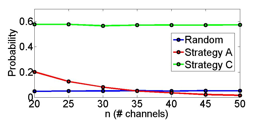
Figure 1: The probability of strategies with $E(TTR)\geq 3n$ in stable environments ($p=0.6$).

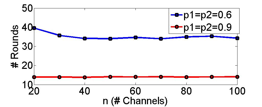
(a) Strategy A ($\lambda=0$)

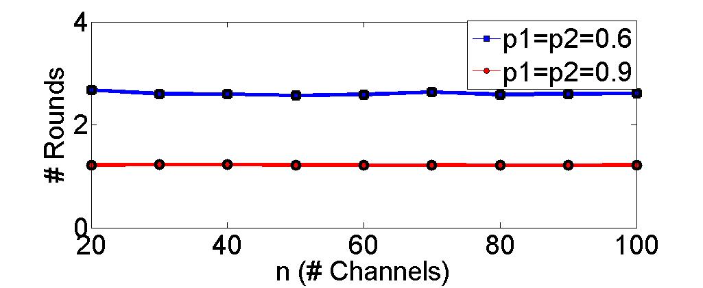
(b) Strategy B ($\lambda=0$)

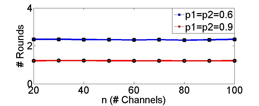
(c) Strategy C ($\lambda=1$)

Figure 2: Performance of strategies with different numbers of channels.

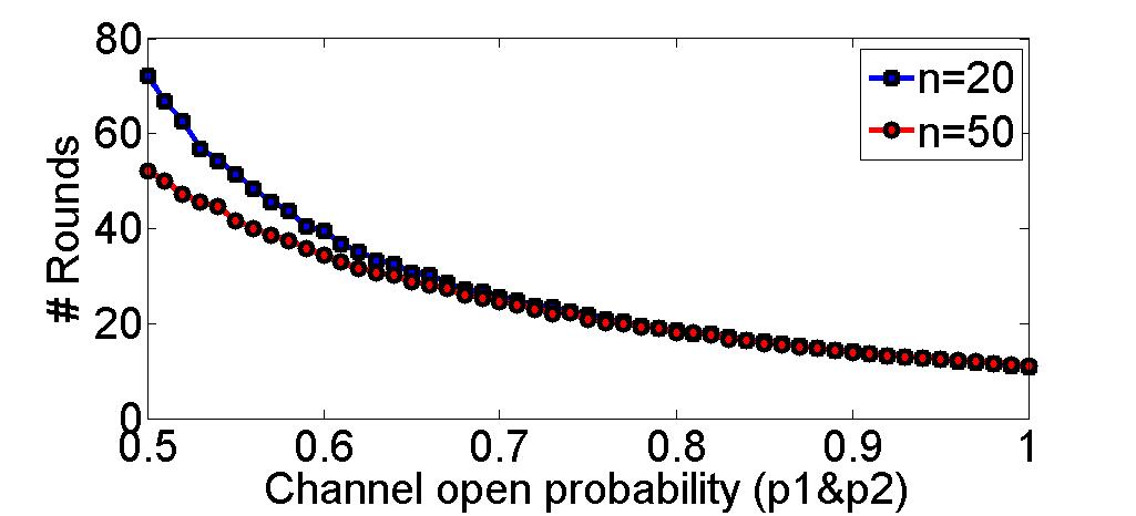
(a) Strategy A ($\lambda=0$)

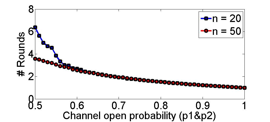
(b) Strategy B ($\lambda=0$)

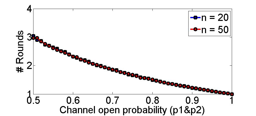
(c) Strategy C ($\lambda=1$)

Figure 3: Performance of strategies with different channel open probabilities.

We can find that our Strategy B can achieve a fast rendezvous and significantly outperforms the random strategy (Random) and Strategy A in stable environments ($\lambda=0$). However, recall that Strategy B needs a common clock. In independent dynamic environments ($\lambda=1$), Strategy C is optimal which validates our theoretical analysis.

Another fact is that, although Strategy A is proved to be optimal in asynchronous stable environments [6], it performs poorly in dynamic environments compared with C which does not need a common clock either, even when $\lambda$ is as small as $0.1$.

In addition, in stable environments, Strategy A may have a bad performance, worse than the random strategy, when $n$ is small (e.g., $n=20$). It is due to the property of the geometric distribution used in Strategy A. We study the the probabilities of $E(TTR)\geq 3n$ for Strategies A, C and Random. Figure 1 shows the results, which validates that Strategy A can not handle cases well when there are only a small number of open channels at Alice and Bob. Moreover, Strategy C always has a high failure probability, which coincides with the fact that Strategy C is not applicable to stable environments.

5.2 Impacts of different parameters

Now, we perform analyses to examine the impacts of different parameters: (1) the channel number $n$; (2) the channel open probability $p$; (3) the environment dynamic factor $\lambda$; and (4) a third party: an intruder.

5.2.1 The channel number $n$

We first examine how the channel number $n$ influences the performance of the strategies. Figure 2 shows the results with different settings of $n$ when $p_{a}=p_{b}=p\in\{0.6,0.9\}$. We can see with relatively large channel open possibilities, the performance is insensitive to $n$. Only Strategy A becomes worse when $n\leq 30$, which is caused by the properties of geometry distribution. In addition, for a larger $p$, the influence of $n$ is smaller. It is reasonable because with a large $p$ there has been plenty of common channels even with a small $n$.

5.2.2 The channel open probabilities $p_{a}$ and $p_{b}$

Figure 3 shows the performance of strategies $A$, $B$ and $C$ with different channel open probabilities. We can see that with the increasing of the open probability, the expected TTR for Strategies A, B and C have a clear decreasing trend, which coincides with our theoretical results stating that the expected time is a reciprocal function of the channel open probability.

5.2.3 The environment dynamic factor

Table 2 has already shown that Strategy C achieves the best performance in independent dynamic environments ($\lambda=1$). Here, we quantitatively examine how the environment dynamic factor $\lambda$ will affect Strategy C. Figure 4 illustrates the performance of Strategy C when $\lambda\in[0.05,1.2]$. We can see the more dynamic the environment is (the closer $\lambda$ approaches to $1$), the better Strategy C performs. It is also straightforward that with larger $p$, the influence of $\lambda$ is smaller as there are plenty of open channels.

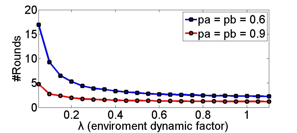
Figure 4: Performance of Strategy C with different environment dynamic factors ($n=30$).

5.2.4 A third party: an intruder

A third party, i.e., an intruder, may block some channels between Alice and Bob. We assume an intruder opens each channel with probability of $q$ and does not change the blocked channels over time. One user does not know a closed channel at his side is due to the existence of the intruder or PUs. Therefore, for the theoretical analysis of rendezvous strategies, this case is equivalent to the environment where there are only Alice and Bob with channel open probabilities of $p_{a}q$ and $p_{b}q$, respectively.

Here, we will examine the influence of an intruder in experiments, and Figure 5 illustrates the results. We can find that 1) The larger the channel open probability is, the smaller influence the intruder causes, which is straightforward; and 2) the existence of an intruder has the largest influence to Strategy A, which is due to the property of geometry distribution used in A.

(a) Strategy A ($\lambda=0$)

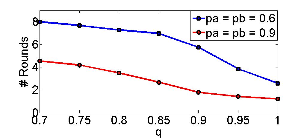
(b) Strategy B ($\lambda=0$)

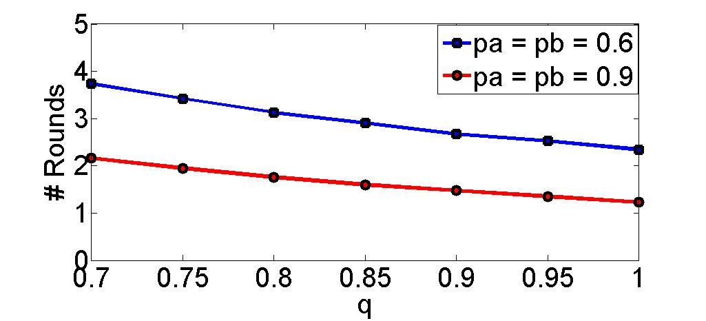
(c) Strategy C ($\lambda=1$)

Figure 5: Performance of strategies with existence of an intruder (n=30).

6 Conclusion

In this paper we study the rendezvous problem in cognitive radio networks. For different system settings, such as asynchronous or synchronous systems in stable or dynamic environments, we derive various strategies and prove their optimality in time-to-rendezvous. Simulations have been carried out to demonstrate the efficiency of our strategies. The impacts of different parameters on the TTR are also investigated. In our current work, each secondary user can only access one channel at a time slot. Designing optimal rendezvous strategies for SUs that can access multiple (continuous) channels at a time is an interesting extension of this work. In addition, to achieve rendezvous among more than two nodes, where there are additional challenges such as the interference between simultaneously transmitting nodes, is also an exciting direction of the future work.

Appendix A Azar et al.’s work

For stable asynchronous environments, Azar et al. proposed in [6] a stationary strategy based on geometric distributions shown as Strategy A:

Strategy A:
At each round,
$\mathcal{S}_{a}$: Alice chooses her $i$-th open channel ($i\geq 1$) with possibility of $\frac{p_{b}}{6}(1-\frac{p_{b}}{6})^{i-1}$.
$\mathcal{S}_{b}$: Bob chooses his $i$-th open channel ($i\geq 1$) with possibility of $\frac{p_{a}}{6}(1-\frac{p_{a}}{6})^{i-1}$.

They also claimed a lower bound of the expected TTR as $\frac{1}{\min(p_{a},p_{b})}$, which holds for any strategies in the stable environments. The proof is trivial. Alice is oblivious of Bob’s channel status. No matter what strategy she uses, at a round, when Alice chooses a channel $i$, the possibility that channel $i$ is open at Bob is $p_{b}$. Therefore, on the side of Alice, the rendezvous possibility at a round is no more than $p_{b}$. A similar result holds for Bob. Then, at each round, the rendezvous probability can not exceed $\min(p_{a},p_{b})$. Therefore, the lower bound is achieved.

Appendix B Proof of Theorem 5

Proof.

We first explain why the argument for the independent dynamic environment is not applicable to the general cases. Take Alice as an example. Given that channel $i$ of Alice is open at time $t$, it will have a probability of $a_{0}=\lambda_{a}(1-p_{a})$ to change to close at time $t+1$. Hence, the open probability of channel $i$ at time $t+1$ is $1-\lambda_{a}(1-p_{a})$, which in general may not be equal to $p_{a}$. Consequently, the events of a channel being open in different time slots are not independent, which makes the previous argument fail when applying to the general cases.

In order to analyze the performance of Strategy C, our idea is to find some special time slots such that, restricted on these slots alone, the environment becomes close to the independent dynamic environment for which a tight upper bound on the TTR has already been obtained. We then argue that such “closeness” can guarantee a similar time upper bound, which gives the desired result.

We now formalize the above idea. Let $R$ be a parameter to be specified later. We restrict Strategy C on the $(jR+1)$-th rounds for all non-negative integers $j$, or equivalently, consider a new strategy $C^{\prime}$ which is identical to $C$ on the $(jR+1)$-th rounds, but in other rounds both Alice and Bob do nothing, i.e., not trying to connect with each other. Obviously the TTR of $C^{\prime}$ is at least as large as that of Strategy $C$. Hence, a proper upper bound on the TTR of $C^{\prime}$ will suffice for our purpose.

For $i\in\{1,2,\ldots,n\}$ and $K,M\geq 1$, let $\mathcal{P}_{i}^{K+M}$ denote the probability that channel $i$ is open for Alice at round $K+M$ given $A_{i}^{K}$, i.e., the availability of channel $i$ for Alice at round $K$. Let $\mathcal{P}_{i}^{K}:=A_{i}^{K}$. (Rigorously speaking $A_{i}^{k}$ is a random variable which takes value 0 or 1. Nonetheless, as shown in the following, the actual value of $A_{i}^{K}$ does not affect the result. Thus we treat $A_{i}^{K}$ as a constant.) Recalling that $a_{0}=\lambda_{a}(1-p_{a})$ and $a_{1}=\lambda_{a}p_{a}$, it is clear that for any integer $M\geq 0$,

$$\mathcal{P}_{i}^{K+M+1} = (1-\lambda_{a}(1-p_{a}))\mathcal{P}_{i}^{K+M}+\lambda_{a}p_{a}(1-\mathcal{P}_{i}^{K+M})$$

$$= (1-\lambda_{a})\mathcal{P}_{i}^{K+M}+\lambda_{a}p_{a}.$$

Rearranging terms gives that for any $M\geq 0$,

$$\mathcal{P}_{i}^{K+M+1}-p_{a}=(1-\lambda_{a})(\mathcal{P}_{i}^{K+M}-p_{a}),$$

from which it follows that

$${\color[rgb]{0,0,0}\mathcal{P}_{i}^{K+R}-p_{a}=(1-\lambda_{a})^{R}(\mathcal{P}_{i}^{K}-p_{a})=(1-\lambda_{a})^{R}(A_{i}^{K}-p_{a}).}$$ (5)

Noting that $(A_{i}^{K}-p_{a})$ is a constant independent of $R$ and that $|1-\lambda_{a}|<1$, we have

$$\mathcal{P}_{i}^{K+R}-p_{a}\rightarrow 0\textrm{~{}~{}as~{}}R\rightarrow+\infty.$$

Therefore, for any $j\geq 1$, the open probability for channel $i$ at round $K+jR$ given its status at round $K$ can be arbitrarily close to $p_{a}$, provided that $R$ is sufficiently large (which can always be guaranteed when $n\rightarrow+\infty$). So the events that channel $i$ is open for Alice at round $jR+1$, for all $j\geq 0$, are “approximately” independent from each other. More precisely, by choosing

$$R=\max\left\{\frac{\ln(1/(0.001p_{a}))}{\ln(1/|1-\lambda_{a}|)},\frac{\ln(1/(0.001p_{b}))}{\ln(1/|1-\lambda_{b}|)}\right\},$$

we can obtain from Eqn (5) that $|\mathcal{P}_{i}^{K+R}-p_{a}|\leq 0.001p_{a}$, which implies that $0.999p_{a}\leq\mathcal{P}_{i}^{K+R}\leq 1.001p_{a}$. (Here the constant 0.001 is just an illustration; it can be arbitrarily small.) Similar results also hold for Bob.

Then, in the $(jR+1)$-th round for each $j\geq 1$, the probability that Alice and Bob both find channel $i$ is at least $(0.999/1.001)^{2}\sum_{i=1}^{n}(1.001p_{a}(1-1.001p_{a})^{i-1})\times(1.001p_{b}(1-1.001p_{b})^{i-1})$, which can be regarded as $(0.999/1.001)^{2}$ times the probability in Eqn (3) with $p_{a}$ and $p_{b}$ replaced with $1.001p_{a}$ and $1.001p_{b}$ respectively. Then, by routine probability calculations similar to Theorem 3, the expected TTR is at most $\left(\frac{1.001}{0.999}\right)^{2}\times\left(\frac{1}{1.001p_{a}}+\frac{1}{1.001p_{b}}-1\right)=O\left(\frac{1}{p_{a}}+\frac{1}{p_{b}}-1\right)$. Finally note that, since only the $(jR+1)$-th rounds are considered, the actually upper bound on the expected TTR should be $R$ times the previous bound. By our choice we have $R=O\left(\ln(1/\min(p_{a},p_{b}))\right)$, as the environment dynamic factors are regarded as constants. ∎

References

- [1] I. F. Akyildiz, W. Lee, M. C. Vuran and S. Mohanty. Next generation/dynamic spectrum access/cognitve radio wireless networks: a survey. Computer Networks, 50(13):2127–2159, 2006.
- [2] S. Alpern, V. J. Baston and S. Essegaier. Rendezvous search on a graph. J. Appl. Probab.., 36(1):223–231, 1999.
- [3] S. Alpern and S. Gal. The theory of search games and rendezvous. International Series in Operations Research & Management Science, 2003. Kluwer Academic Publishers.
- [4] S. Alpern and M. Pikounis. The telephone coordination game. Game theory and applications. L.A. Petrosjan and V.V. Mazalov (Eds.), Nova Science Publishers Incorporated, Huntington, New York, USA.
- [5] E. J. Anderson and R. R. Weber. The rendezvous problem on discrete locations. J. Appl. Probab., 27(4):839–851, 1990.
- [6] Y. Azar1, O. Gurel-Gurevich, E. Lubetzky and T. Moscibroda. Optimal discovery strategies in white space networks. In Proc. ESA, 2011.
- [7] P. Bahl, R. Chandra, T. Moscibroda, R. Murty and M. Welsh. White space networking with Wi-Fi like connectivity. In Proc. ACM SIGCOMM, 2009.
- [8] C. Cordeiro, K. Challapali, D. Birru and S. S. N. IEEE 802.22: the first worldwide wireless standard based on cognitive radios. J. of Communications, 1(1):38–47, 2006.
- [9] R. Gandhi, C.-C. Wang, Y.C. Hu. Fast rendezvous for multiple clients for cognitive radios using coordinated channel hopping. In Proc. IEEE SECON, 2012.
- [10] J. Jia, Q. Zhang and X. Shen. HC-MAC: a hardware-constrained cognitive MAC for efficient spectrum management. IEEE J. on Selected Areas in Communications, 26(1):106–117, 2008.
- [11] X.-Y. Li, P. Yang, Y. Yan, L. You, S. Tang and Q. Huang. Almost optimal accessing of nonstochastic channels in cognitive radio networks. In Proc. 31st IEEE INFOCOM, pages 2291–2299, 2012.
- [12] Z. Lin, H. Liu, X. Chu and Y.-W. Leung. Jump-stay based channelhopping algorithm with guaranteed rendezvous for cognitive radio networks. In Proc. IEEE INFOCOM, pages 2444–2452, 2011.
- [13] D. Lu, X. Huang, P. Li and J. Fan. Connectivity of large-scale cognitive radio ad hoc networks. In Proc. 31st IEEE INFOCOM, pages 1260–1268, 2012.
- [14] D. Meier, Y.-A. Pignolet-Oswald, S. Schmid and R. Wattenhofer. Speed Dating despite Jammers. In Proc. DCOSS, 2009.
- [15] J. Pérez-Romero, O. Sallent, R. Agustí and L. Giupponi. A novel ondemand cognitive pilot channel enabling dynamic spectrum allocation. In Proc. IEEE DySpan, pp. 46–54 2007.
- [16] W. Ren, Q. Zhao and A. Swami. Power control in cognitive radio networks: How to cross a multi-lane highway. IEEE J. on Selected Areas in Communications, 27(7):1283–1296, 2009.
- [17] S. Romaszko, D. Denkovski, V. Pavlovska and L. Gavrilovska. Asynchronous Rendezvous Protocol for Cognitive Radio Ad Hoc Networks. In Ad Hoc Networks, Vol. 111, pp. 135–148, 2013
- [18] G. Taricco. Optimization of Linear Cooperative Spectrum Sensing for Cognitive Radio Networks. IEEE J. of Selected Topics in Signal Processing, 5(1):77–86, 2011.
- [19] N. C. Theis, R. W. Thomas, and L. A. DaSilva. Rendezvous for cognitive radios. IEEE Trans. on Mobile Computing, 10(2):216–227, 2011.
- [20] C. Xu and J. Huang. Spatial spectrum access game: nash equilibria and distributed learning. In Proc. ACM MobiHoc, 2012.
- [21] Y. Yuan, P. Bahl, R. Chandra, T. Moscibroda and Y. Wu. Allocating dynamic time-spectrum blocks in cognitive radio networks. In Proc. ACM MobiCom, pp. 130–139, 2007.
- [22] J. Zhao, H. Zheng and G.-H. Yang. Distributed coordination in dynamic spectrum allocation networks. In Proc. IEEE DySpan, pp. 259–268, 2005.