Compressive Origin-Destination Estimation

Abstract

The paper presents an approach to estimate Origin-Destination (OD) flows and their path splits, based on traffic counts on links in the network. The approach called Compressive Origin-Destination Estimation (CODE) is inspired by Compressive Sensing (CS) techniques. Even though the estimation problem is underdetermined, CODE recovers the unknown variables exactly when the number of alternative paths for each OD pair is small. Noiseless, noisy, and weighted versions of CODE are illustrated for synthetic networks, and with real data for a small region in East Providence. CODE’s versatility is suggested by its use to estimate the number of vehicles and the Vehicle-Miles Traveled (VMT) using link counts.

I Introduction

A common task in transportation planning is to estimate path allocations, that is the Origin-Destination (OD) flows and the path splits for each flow, from traffic counts on individual links in a network[1, 2, 3, 4, 5, 6, 7, 8]. (Estimation using tag data from Automatic Vehicle Identification (AVI) and Electronic Toll Collection (ETC) is discussed in [9, 10, 11, 12].) One may use static or dynamic traffic models [13, 14, 7]. In a static model the flows and link counts are time-independent. In a dynamic model the flows and link counts are time-dependent[1, 15, 16, 3, 17, 18].

The unknown path allocation vector $\boldsymbol{x}$ contains all OD pair flows and path splits for each OD pair. The problem is to recover $\boldsymbol{x}\in\mathbb{R}^{N}$ from the link count measurement vector $\boldsymbol{y}\in\mathbb{R}^{M}$ when $N$ is much larger than $M$. The two vectors are related by $\boldsymbol{y}=A\boldsymbol{x}$ in which $A$ is the known binary incidence matrix that specifies the links along each path. We approach the problem supposing that $\boldsymbol{x}$ is sparse, i.e., the number $S$ of non-zero entries in $\boldsymbol{x}$ is much smaller than $N$. The approach called Compressive Origin-Destination Estimation (CODE) is inspired by Compressive Sensing (CS)[19, 20, 21] techniques developed in signal processing for sparse signal recovery. We show that CODE recovers the path allocation vector $\boldsymbol{x}$ when it is suitably sparse. The main technical novelty of our approach is to formulate the estimation problem as $\ell_{1}$-recovery of a sparse signal $x$.

Our motivation behind imposing the sparsity condition on $\boldsymbol{x}$ is due to the fact that in a typical urban area there are many possible paths between any given OD pair while only a small fraction of these paths are plausible to the travelers based on travel length, travel time, number of turns, etc. CODE assumes that the plausible paths between any given OD pair is sparse. We give a brief example as to why sparsity is likely. Consider a grid square network with nodes indexed $(m,n)$ from bottom-left to the top-right of the grid. Links only go west to east or south to north. The most bottom-left node (origin) is (0,0) and the most top-right node (destination) is $(N/2,N/2)$. There are $N\choose N/2$ possible paths that connects origin (0,0) to destination $(N/2,N/2)$. For example, for $N=50$ there exist $1.2641\times 10^{+14}$ possible paths. While each path traverses N links (i.e., all paths have the same length), it may contain different number of turns. For example, there only exist two paths with just 1 turn. The fraction of paths that make at most $\alpha N$ turns is bounded using the Hoeffding’s inequality by $\beta=\exp(-2(0.5-\alpha)^{2}N)$. Suppose we believe that drivers will not take a route with more than $0.1N$ turns ($\alpha=0.1$). For $N=50$ the fraction of plausible routes with at most $5$ turns is less than $10^{-7}$ of all possible routes. If they won’t take routes with more than $0.2N$ turns ($\alpha=0.2$), the fraction of all plausible routs with at most $10$ turns is at most $10^{-4}$. The ratio $\beta$ is small and will decrease as N increases, motivating the sparsity assumption on $\boldsymbol{x}$.

In section II, we formulate the problem for both static and dynamic models and introduce the sparse path allocation framework. We list basic tools of CS and $\ell_{1}$-minimization in section III. We introduce CODE in its noiseless and noisy settings with a small example in section IV. A weighted version of CODE is examined in section V. In Section VI we consider the Nguyen-Dupuis network and show how the proposed framework can be used to estimate Vehicle-Miles Traveled (VMT). A study based on data taken from a traffic area in East Providence is presented in section VII.

II Problem Setup

Consider a traffic network like in Fig. 1 with nodes or zones indexed $i,j$ and unidirectional links $\ell_{j}^{i}$ from $i$ to $j$.

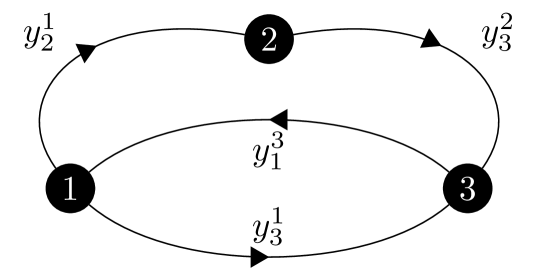
Figure 1: Traffic network with 3 OD zones, 4 links, and 7 possible paths associated with 6 possible OD pairs. In this example, for each OD pair there is only one path except for OD pair 1-3 which has 2 alternative paths: $\ell_{2}^{1}\ell_{3}^{2}$ and $\ell_{3}^{1}$.

An OD pair might be connected by several alternative paths. For example, from origin $2$ to destination $1$ there is a single path that traverses nodes $2\rightarrow 3\rightarrow 1$, while from origin $1$ to destination $3$ there are two paths: $1\rightarrow 3$ and $1\rightarrow 2\rightarrow 3$. The number of vehicles $y_{j}^{i}$ that pass through link $\ell_{j}^{i}$ is measured so, for example,

$$y_{2}^{1}=x^{\ell^{1}_{2}}+x^{\ell^{1}_{2}\ell^{2}_{3}}+x^{\ell^{3}_{1}\ell^{1}_{2}}:=x_{1}+x_{2}+x_{7},$$

in which $x^{p_{i}}$ (also written $x_{i}$) is the number of vehicles that take path $p_{i}$. In this example there are seven possible paths associated with six different OD pairs. The vector $y$ of traffic counts is a linear function of the vector $x$ of path flows:

$$\underbrace{\begin{bmatrix}y_{2}^{1}\\ y_{3}^{1}\\ y_{3}^{2}\\ y_{1}^{3}\end{bmatrix}}_{\boldsymbol{y}}=\underbrace{\begin{bmatrix}1&1&0&0&0&0&1\\ 0&0&1&0&0&0&0\\ 0&1&0&1&1&0&0\\ 0&0&0&1&0&1&1\\ \end{bmatrix}}_{A}\underbrace{\begin{bmatrix}x_{1}\\ x_{2}\\ x_{3}\\ x_{4}\\ x_{5}\\ x_{6}\\ x_{7}\\ \end{bmatrix}}_{\boldsymbol{x}}.$$ (1)

The matrix element $A_{ij}=1$ or $0$ accordingly as link $i$ belongs to path $j$ or not. The goal is to recover the path allocations $\boldsymbol{x}$ from observed link counts $\boldsymbol{y}$. Since this is an underdetermined set of of linear equations unique recovery of the true solution is generally not possible. However we show that under sparsity conditions on the true $\boldsymbol{x}$ we can recover a unique solution. We describe the traffic model next.

II-A Static Model

There are $K$ OD pairs ($k=1,2,\dots,K$) and $N$ paths ($n=1,2,\dots,N$). $y^{i}_{j}$ is the vehicle count on link $\ell^{i}_{j}$ and $f_{k}$ is the flow over the $k$th OD pair. The measurement model is

$$y^{i}_{j}=\sum_{k}\left(\sum_{n}w_{k,n}a^{i\to j}_{k,n}\right)f_{k},$$ (2)

where $w_{k,n}$ is the fraction of the flow $f_{k}$ over the $k$th OD pair that takes the $n$th path, and $a^{i\to j}_{k,n}=1$ if $\ell^{i}_{j}$ belongs to the $n$th path in the $k$th OD pair and $=0$ otherwise [22]. The weights or path splits $w_{k,n}$ satisfy

$$\sum_{n}w_{k,n}=1,\;\;0\leq w_{k,n}\leq 1.$$ (3)

We reformulate the measurement equation (2) as

$$y^{i}_{j}=[a^{i\to j}_{1,1}\dots a^{i\to j}_{k,n}\dots a^{i\to j}_{K,N}]\underbrace{\begin{bmatrix}w_{1,1}f_{1}\\ \vdots\\ w_{k,n}f_{k}\\ \vdots\\ w_{K,N}f_{K}\end{bmatrix}}_{\boldsymbol{x}\in\mathbb{R}^{N}}.$$ (4)

In (4) the dimension of the unknown vector $\boldsymbol{x}$ is the number of paths in a network.

For Fig. 1, define $p_{1}=\ell^{1}_{2},p_{2}=\ell^{1}_{2}\ell^{2}_{3},p_{3}=\ell^{1}_{3},p_{4}=\ell^{2}_{3}\ell^{3}_{1},p_{5}=\ell^{2}_{3},p_{6}=\ell^{3}_{1},p_{7}=\ell^{3}_{1}\ell^{1}_{2}$. From (3), $w_{1,1}=w_{3,4}=w_{4,5}=w_{5,6}=w_{6,7}=1$ and $w_{2,2}+w_{2,3}=1$, so the measurement equation becomes

$$\left\{\begin{array}[]{ll}y^{1}_{2}&=\underbrace{w_{1,1}f_{1}}_{x_{1}}+\underbrace{w_{2,2}f_{2}}_{x_{2}}+\underbrace{w_{6,7}f_{6}}_{x_{7}}=f_{1}+w_{2,2}f_{2}+f_{6},\\ y^{1}_{3}&=\underbrace{w_{2,3}f_{2}}_{x_{3}}=w_{2,3}f_{2},\\ y^{2}_{3}&=\underbrace{w_{2,2}f_{2}}_{x_{2}}+\underbrace{w_{3,4}f_{3}}_{x_{4}}+\underbrace{w_{4,5}f_{4}}_{x_{5}}=w_{2,2}f_{2}+f_{3}+f_{4},\\ y^{3}_{1}&=\underbrace{w_{3,4}f_{3}}_{x_{4}}+\underbrace{w_{5,6}f_{5}}_{x_{6}}+\underbrace{w_{6,7}f_{6}}_{x_{7}}=f_{3}+f_{5}+f_{6}.\end{array}\right.$$ (5)

Remark 1

If CODE recovers $\boldsymbol{x}$, one also obtains the OD flows $f_{k}$ and path splits $w_{k,n}$. For example, given $x_{2}$ and $x_{3}$, we can recover $f_{2}$ because $x_{2}+x_{3}=w_{2,2}f_{2}+w_{2,3}f_{2}=(w_{2,2}+w_{2,3})f_{2}=f_{2}$. We also recover $w_{2,2}=x_{2}/f_{2}$ and $w_{2,3}=x_{3}/f_{2}$.

Remark 2

In the measurement equation (4) the unknown weights $w_{k,n}$ are incorporated into $\boldsymbol{x}$. This is different from studies in which these weights are known a priori. Our approach increases the dimension of the unknown vector $\boldsymbol{x}$. However, when $\boldsymbol{x}$ is suffiiciently sparse, it can be recovered by CODE. Of course, if some flows and weights are known, these values can replace the corresponding variables.

II-B Dynamic Traffic Model

In a dynamic model, the OD flows $f_{k}$ and link counts $y^{i}_{j}$ are time-dependent, e.g., hourly. More significantly, we need to account for the time delay between the start time of a vehicle’s trip and the count time when its presence on a link is measured. To illustrate how the measurement equation (4) changes, we consider the network of Fig. 1, assuming it takes one unit time to traverse each link, so that

$$\left\{\begin{array}[]{ll}y^{1}_{2}(t)&=f_{1}(t)+w_{2,2}f_{2}(t)+f_{6}(t-1),\\ y^{1}_{3}(t)&=w_{2,3}f_{2}(t),\\ y^{2}_{3}(t)&=w_{2,2}f_{2}(t-1)+f_{3}(t)+f_{4}(t),\\ y^{3}_{1}(t)&=f_{3}(t-1)+f_{5}(t)+f_{6}(t).\end{array}\right.$$ (6)

In matrix form (6) is written as

$$\boldsymbol{y}(t)=\underbrace{\begin{bmatrix}1&1&0&0&0&0&0&0&0&1\\ 0&0&1&0&0&0&0&0&0&0\\ 0&0&0&1&1&0&1&0&0&0\\ 0&0&0&0&0&1&0&1&1&0\\ \end{bmatrix}}_{A}\underbrace{\begin{bmatrix}f_{1}(t)\\ w_{2,2}f_{2}(t)\\ w_{2,3}f_{2}(t)\\ w_{2,2}f_{2}(t-1)\\ f_{3}(t)\\ f_{3}(t-1)\\ f_{4}(t)\\ f_{5}(t)\\ f_{6}(t)\\ f_{6}(t-1)\end{bmatrix}}_{\boldsymbol{x}(t)}$$ (7)

where $\boldsymbol{y}(t)=[y_{2}^{1}(t),y_{3}^{1}(t),y_{3}^{2}(t),y_{1}^{3}(t)$. Evidently, considering time delays increases the dimension of the unknown $\boldsymbol{x}(t)$. But if a time-series is observed there will be more measurements as well.

III Compressive Sensing (CS)

CS techniques [23, 19] are used to recover an unknown signal $\boldsymbol{x}\in\mathbb{R}^{N}$ from observations $\boldsymbol{y}=A\boldsymbol{x}\in\mathbb{R}^{M}$ ($M\ll N$) when $x$ is sparse, i.e. the number of non-zero entries of $\boldsymbol{x}$, $S\ll N$. $S:=\|\boldsymbol{x}\|_{0}$ denotes the sparsity level of $\boldsymbol{x}$. Since $M<N$ there are infinitely many candidate solutions to $\boldsymbol{y}=A\boldsymbol{x}$ for a given $\boldsymbol{y}$. Recovery of $\boldsymbol{x}$ is nonetheless possible if the true signal is sparse. The recovery algorithm seeks a sparse solution among the candidates.

III-A Recovery via $\ell_{0}$-minimization

Recovery of a sparse $\boldsymbol{x}$ can be formulated via $\ell_{0}$-minimization

$$\widehat{\boldsymbol{x}}_{\ell_{0}}:=\arg\min\|\boldsymbol{x}\|_{0}\ \ \ \ \ \text{subject to}\ \ \ \ \ \boldsymbol{y}=A\boldsymbol{x}.$$ (8)

Problem (8) can be interpreted as finding an $S$-term approximation to $\boldsymbol{y}$ given $A$ [19].

III-B Recovery via $\ell_{1}$-minimization

The $\ell_{0}$-minimization problem (8) is NP-hard. Results of CS indicate that it is not always necessary to solve the $\ell_{0}$-minimization problem (8) to recover $\boldsymbol{x}$, and a much simpler problem often yields an equivalent solution: we only need to find the “$\ell_{1}$-sparsest” $\boldsymbol{x}$ by solving

$$\widehat{\boldsymbol{x}}_{\ell_{1}}:=\arg\min\|\boldsymbol{x}\|_{1}\ \ \ \ \ \text{subject to}\ \ \ \ \ \boldsymbol{y}=A\boldsymbol{x}.$$ (9)

The $\ell_{1}$-minimization problem (9), called Basis Pursuit [24], is much simpler and can be solved as a linear program whose computational complexity is polynomial in $N$. A ‘noise-aware’ version of the $\ell_{1}$-minimization (9) relaxes the equality constraint as

$$\widehat{\boldsymbol{x}}_{\ell_{1}}:=\arg\min\|\boldsymbol{x}\|_{1}\ \ \ \ \ \text{subject to}\ \ \ \ \ \|\boldsymbol{y}-A\boldsymbol{x}\|_{2}\leq\delta,$$ (10)

where $\delta$ is a parameter that should increase with measurement noise.

III-C $\ell_{0}/\ell_{1}$ Equivalence and the Restricted Isometry Property

Of course $\widehat{\boldsymbol{x}}_{\ell_{1}}$ is not equal to $\widehat{\boldsymbol{x}}_{\ell_{0}}$ without conditions on $A$. The Restricted Isometry Property (RIP) [25, 21] guarantees that the $\ell_{1}$-minimizing solution is equivalent to the $\ell_{0}$-minimizing solution. But RIP is only a sufficient condition and frequently the $\ell_{1}$-minimization recovers the true sparse solution even without RIP. The gap between existing recovery guarantees and actual recovery performance is being narrowed in different applications. In particular, when sparse dynamical systems are involved this gap is usually large and has been investigated in system identification [26, 27, 28, 29, 30], observability and control of linear systems [31, 32], and identification of interconnected networks [33, 34].

IV A Traffic Network Example

To explain the ideas, consider the static model for the network of Figure 2 with $4$ nodes (OD zones) and 10 links. Each of the 12 possible OD pairs has alternative paths. We assume that only 3 of the OD pairs are plausible. Table I lists these 3 OD pairs and their corresponding 14 paths. When all 10 link counts are available the measurement equation is

$$\boldsymbol{y}=$$

TABLE I: The 3 plausible OD pairs and their corresponding 14 paths for the network of Fig. 2.

$$\begin{array}[]{c||c||c|c||c|c}\hline\cr\hline\cr&\color[rgb]{0,0,1}{\text{OD pair}}\ \ 3-1&&\color[rgb]{0,0,1}{\text{OD pair}}\ \ 3-2&&\color[rgb]{0,0,1}{\text{OD pair}}\ \ 4-2\\ \hline\cr\color[rgb]{0,0,1}{p_{1}}&\ell^{3}_{1}&\color[rgb]{0,0,1}{p_{6}}&\ell^{3}_{1}\to\ell^{1}_{2}&\color[rgb]{0,0,1}{p_{10}}&\ell^{4}_{1}\to\ell^{1}_{2}\\ \hline\cr\color[rgb]{0,0,1}{p_{2}}&\ell^{3}_{2}\to\ell^{2}_{1}&\color[rgb]{0,0,1}{p_{7}}&\ell^{3}_{2}&\color[rgb]{0,0,1}{p_{11}}&\ell^{4}_{1}\to\ell^{1}_{3}\to\ell^{3}_{2}\\ \hline\cr\color[rgb]{0,0,1}{p_{3}}&\ell^{3}_{2}\to\ell^{2}_{4}\to\ell^{4}_{1}&\color[rgb]{0,0,1}{p_{8}}&\ell^{3}_{4}\to\ell^{4}_{1}\to\ell^{1}_{2}&\color[rgb]{0,0,1}{p_{12}}&\ell^{4}_{2}\\ \hline\cr\color[rgb]{0,0,1}{p_{4}}&\ell^{3}_{4}\to\ell^{4}_{1}&\color[rgb]{0,0,1}{p_{9}}&\ell^{3}_{4}\to\ell^{4}_{2}&\color[rgb]{0,0,1}{p_{13}}&\ell^{4}_{3}\to\ell^{3}_{1}\to\ell^{1}_{2}\\ \hline\cr\color[rgb]{0,0,1}{p_{5}}&\ell^{3}_{4}\to\ell^{4}_{2}\to\ell^{2}_{1}&&&\color[rgb]{0,0,1}{p_{14}}&\ell^{4}_{3}\to\ell^{3}_{2}\\ \hline\cr\hline\cr\end{array}$$

$$\underbrace{\setcounter{MaxMatrixCols}{14}\begin{bmatrix}0&0&0&0&0&1&0&1&0&1&0&0&1&0\\ 0&0&0&0&0&0&0&0&0&0&1&0&0&0\\ 0&1&0&0&1&0&0&0&0&0&0&0&0&0\\ 0&0&1&0&0&0&0&0&0&0&0&0&0&0\\ 1&0&0&0&0&1&0&0&0&0&0&0&1&0\\ 0&1&1&0&0&0&1&0&0&0&1&0&0&1\\ 0&0&0&1&1&0&0&1&1&0&0&0&0&0\\ 0&0&1&1&0&0&0&1&0&1&1&0&0&0\\ 0&0&0&0&1&0&0&0&1&0&0&1&0&0\\ 0&0&0&0&0&0&0&0&0&0&0&0&1&1\\ \end{bmatrix}}_{A\in\mathbb{R}^{10\times 14}}\underbrace{\begin{bmatrix}w_{1,1}f_{1}\\ w_{1,2}f_{1}\\ w_{1,3}f_{1}\\ w_{1,4}f_{1}\\ w_{1,5}f_{1}\\ w_{2,6}f_{2}\\ w_{2,7}f_{2}\\ w_{2,8}f_{2}\\ w_{2,9}f_{2}\\ w_{3,10}f_{3}\\ w_{3,11}f_{3}\\ w_{3,12}f_{3}\\ w_{3,13}f_{3}\\ w_{3,14}f_{3}\\ \end{bmatrix}}_{\boldsymbol{x}\in\mathbb{R}^{14}}.$$ (11)

where $\boldsymbol{y}=[y_{2}^{1},y_{3}^{1},y_{1}^{2},y_{4}^{2},y_{1}^{3},y_{2}^{3},y_{4}^{3},y_{1}^{4},y_{2}^{4},y_{3}^{4}]\in\mathbb{R}^{10}$.

One common way to recover $\boldsymbol{x}$ is via $\ell_{2}$-minimization:

$$\widehat{\boldsymbol{x}}_{\ell_{2}}:=\arg\min\|\boldsymbol{x}\|_{2}\ \ \ \ \ \text{subject to}\ \ \ \left\{\begin{array}[]{cc}\boldsymbol{y}=A\boldsymbol{x}\\ x_{i}\geq 0,\forall i.\end{array}\right.$$ (12)

This is one of several ‘least-squares’ estimation techniques studied in the literature [5, 7, 8]. We will compare $\widehat{\boldsymbol{x}}_{\ell_{2}}$ and $\widehat{\boldsymbol{x}}_{\ell_{1}}$:

$$\widehat{\boldsymbol{x}}_{\ell_{1}}:=\arg\min\|\boldsymbol{x}\|_{1}\ \ \ \ \ \text{subject to}\ \ \ \left\{\begin{array}[]{cc}\boldsymbol{y}=A\boldsymbol{x}\\ x_{i}\geq 0,\forall i.\end{array}\right.$$ (13)

The constraint $x_{i}\geq 0,\forall i$ ensures that the path allocations are non-negative. (Such non-negativity constraints are not usually present in CS.)

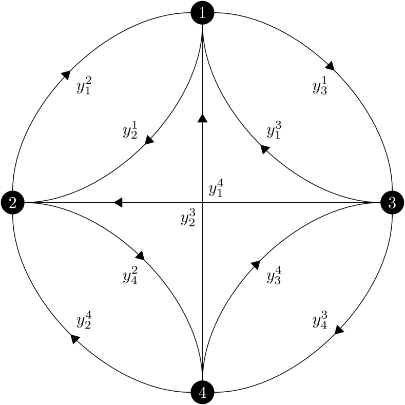
Figure 2: Traffic network with 4 OD zones and 10 links.

IV-A Noiseless Recovery of Sparse Path Allocations

We consider several scenarios in which $\ell_{1}$-minimization (13) successfully recovers $\boldsymbol{x}$ for the network of Fig. 2.

Example 1 ($\ell_{1}$-Recovery vs. $\ell_{2}$-Recovery)

Suppose we have only $6$ link measurements: $\{y^{1}_{2},y^{1}_{3},y^{2}_{1},y^{3}_{2},y^{3}_{4},y^{4}_{3}\}$. The goal is to recover $\boldsymbol{x}\in\mathbb{R}^{14}$ based on these measurements. The true path allocation $\boldsymbol{x}$ is $4$-sparse. Specifically $p_{2}$ is used by OD pair $3-1$ with $w_{1,2}=1$, $p_{8}$ by OD pair $3-2$ with $w_{2,8}=1$, and $p_{11}$ and $p_{14}$ are taken by OD pair $4-2$ with $w_{3,11}=0.25$ and $w_{3,14}=0.75$. Fig. 3 depicts the recovery results: $\ell_{1}$-minimization recovers the true $4$-sparse $\boldsymbol{x}\in\mathbb{R}^{14}$ from the $6$ link measurements while $\ell_{2}$-minimization fails, which motivates CODE. As expected the least squares estimate is not sparse.

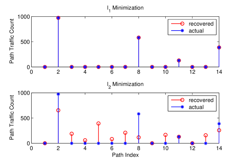
Figure 3: (Example 1) Illustration of how $\ell_{1}$-minimization succeeds and $\ell_{2}$-minimization fails to recover the true $4$-sparse path allocation from 6 link flow measurements of the traffic network of Fig. 2.

Example 2

We show that the required number of measurements for exact recovery via $\ell_{1}$-minimization increases with the sparsity level of $\boldsymbol{x}$. Consider two fixed supports for $\boldsymbol{x}$: a 3-sparse $\boldsymbol{x}$ ($\mathcal{S}_{1}=\{5,9,13\}$) and a 4-sparse $\boldsymbol{x}$ ($\mathcal{S}_{2}=\{2,8,11,14\}$). For each support, we generate several $\boldsymbol{x}$ satisfying (3), and repeat this experiment for different number of link flow measurements. For each fixed number of measurements, we randomly choose a subset of link flow measurements. For each of 500 trials we solve the $\ell_{1}$-minimization (13).

In order to better characterize the recovered solutions, we consider three different recovery criteria. The strictest criterion requires $\widehat{\boldsymbol{x}}_{\ell_{1}}=\boldsymbol{x}$, so all path splits and OD flows are perfectly estimated. In the second criterion $\widehat{\boldsymbol{x}}_{\ell_{1}}$ is a successful recovery if all OD flows are perfectly recovered while the path splits may not be correctly estimated. The weakest criterion only requires the sum of all OD flows to match the true total flow sum, i.e. the total number of vehicles is correctly estimated, while the OD flows and path split estimates may have errors. These criteria may be appropriate depending on the application. Fig. 4 summarizes the recovery results. Fig. 4 and 4 depict how the performance improves as the recovery criterion is relaxed for a $3$-sparse and a $4$-sparse $\boldsymbol{x}$, respectively. As expected, more measurements are needed to recover a $4$-sparse $\boldsymbol{x}$ than a $3$-sparse $\boldsymbol{x}$.

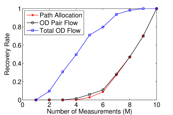
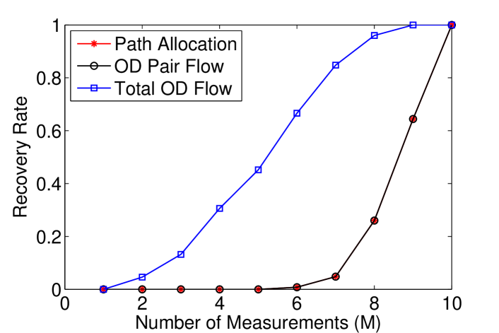
Figure 4: (Example 2) Illustration of how the recovery rate changes with measurements. Two fixed supports (3- and 4-sparse) are considered. In order to better characterize the recovered solutions, three different recovery criteria (path allocation recovery, OD flow recovery, and total OD flow recovery) are considered. (a) 3-sparse path allocation. (b) 4-sparse path allocation.

Example 3

We consider all possible $3$-, 4-, and 5-sparse signals and for each, we calculate the recovery rate for different number $M$ of measurements over 500 trials. The results are illustrated in Fig. 5. At each iteration and for a given sparsity level $S$, we randomly generate a signal $\boldsymbol{x}$ (with random OD flow values and weights while satisfying (3) and on a random support). We then randomly select the link flow measurements for a given $M$. For each pair of $M$ and $S$, we repeat this procedure for 500 iterations and calculate the recovery rate as the fraction of times that there is an exact recovery (based on the strictest recovery criterion) via $\ell_{1}$-minimization.

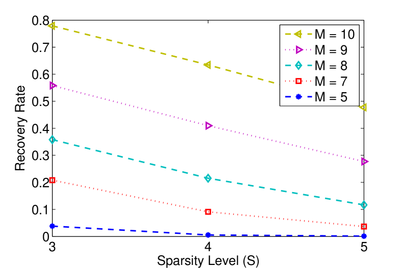
Figure 5: (Example 3) Illustration of how the recovery rate changes with sparsity and measurements. We perform the following procedure at each iteration. For a given sparsity level and number of measurements, we randomly select the support and generate $\boldsymbol{x}$, calculate $\boldsymbol{y}$, and then randomly choose a subset of links as our available measurements. For each pair $(S,M)$, we repeat this procedure for 500 iterations and calculate the recovery rate as the fraction of times there is an exact recovery by solving the $\ell_{1}$-minimization.

IV-B Noisy CODE and Compressible Path Allocations

The ideal case of a sparse signal with noiseless measurements rarely occurs in practice. One usually deals with compressible signals and noisy measurements, A signal $\boldsymbol{x}\in\mathbb{R}^{N}$ is said to be compressible when it has more than $S<N$ non-zero entries but can be well approximated by its $S$ largest entries.

Example 4 (Noisy $\ell_{1}$-Recovery)

We illustrate CODE for noisy measurements. As in Example 2 we consider a 3-sparse and a 4-sparse signal and $M=10$ link measurements to which are added Gaussian noises with distribution $\mathcal{N}(0,0.1^{2})$ for the 3-sparse signal and distribution $\mathcal{N}(0,0.02^{2})$ for the 4-sparse signal. We use a noise-aware version of (13):

$$\widehat{\boldsymbol{x}}_{\ell_{1}}:=\arg\min\|\boldsymbol{x}\|_{1}\ \ \text{subject to}\ \ \left\{\begin{array}[]{cc}\|\boldsymbol{y}-A\boldsymbol{x}\|_{2}\leq\delta\\ x_{i}\geq 0,\forall i.\end{array}\right.$$ (14)

The parameter $\delta$ depends on the measurement noise. We compare the estimates of (14) with a noise-aware version of the $\ell_{2}$-minimization (12):

$$\widehat{\boldsymbol{x}}_{\ell_{2}}:=\arg\min\|\boldsymbol{x}\|_{2}\ \ \text{subject to}\ \ \left\{\begin{array}[]{cc}\|\boldsymbol{y}-A\boldsymbol{x}\|_{2}\leq\delta\\ x_{i}\geq 0,\forall i.\end{array}\right.$$ (15)

Fig. 6 and 6 illustrate the noisy recovery results where we plot the empirical Cumulative Distribution Function (CDF) of recovery error $\|\widehat{\boldsymbol{x}}-\boldsymbol{x}\|_{2}/\|\boldsymbol{x}\|_{2}$ over $1000$ iterations, for 3- and 4-sparse signals, respectively. As can be seen, $\ell_{1}$-minimization is much less sensitive to noise and has a much smaller recovery error $\|\widehat{\boldsymbol{x}}-\boldsymbol{x}\|_{2}/\|\boldsymbol{x}\|_{2}$ in both cases.

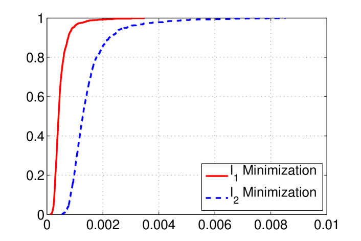
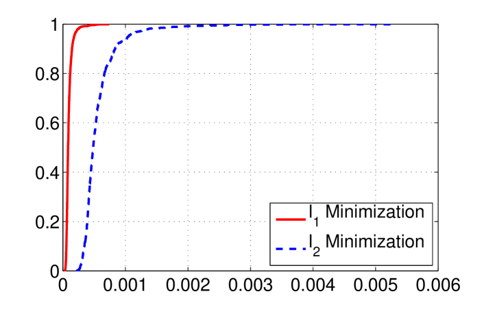
Figure 6: (Example 4) CODE from noisy measurements. Two fixed supports (a 3-sparse and a 4-sparse) are considered as in Example 2. All $M=10$ link measurements are available. A Gaussian noise with $\mathcal{N}(0,\nu^{2})$ is added to true measurements. We plot the empirical CDF of the error over $1000$ iterations. (a) 3-sparse with $\nu=0.1$ (b) 4-sparse with $\nu=0.02$.

V Weighted $\ell_{1}$-Minimization

Additional knowledge, for example on AVI or ETC tag data, can improve recovery of the true path allocation vector $\boldsymbol{x}$ by using a weighted version of the $\ell_{1}$-minimization problem (13):

$$\widehat{\boldsymbol{x}}_{w}=\arg\min\|\Lambda\boldsymbol{x}\|_{1}\ \ \ \ \ \text{subject to}\ \ \ \ \ \left\{\begin{array}[]{cc}\boldsymbol{y}=A\boldsymbol{x}\\ x_{i}\geq 0,\forall i,\end{array}\right.$$ (16)

where $\Lambda\in\mathbb{R}^{N\times N}$ is a given diagonal matrix with positive entries (weights) on the diagonal. Since $\|\Lambda\boldsymbol{x}\|_{1}=\sum_{i}\lambda_{i}|x_{i}|$ is a weighted sum of the entries of $\boldsymbol{x}$, this is also a linear program. An entry of $\boldsymbol{x}$ assigned a large weight gets more penalized in the minimization problem.

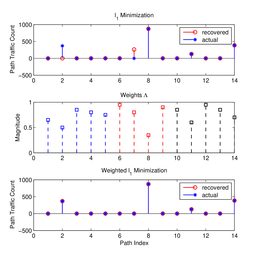
Figure 7: Illustration of how weighted $\ell_{1}$-minimization can help recovery of a $4$-sparse path allocation $\boldsymbol{x}\in\mathbb{R}^{14}$ from 6 link flow measurements of the traffic network given in Fig. 2.

Fig. 7 shows an example where incorporating extra information in CODE improves the recovery of a 4-sparse $\boldsymbol{x}$ from 6 link flow measurements $\{y^{1}_{2},y^{1}_{3},y^{3}_{2},y^{3}_{4},y^{4}_{2},y^{4}_{3}\}$ using weighted $\ell_{1}$-minimization (16). The weights are chosen based on our prior knowledge of the path allocations. For example, for OD pair $3-1$, a smaller weight is assigned to the entry associated with the true path ($p_{2}$) compared to other alternative paths for this OD pair. Similarly, smaller weights are assigned to entries $8$, $11$, and $14$, forcing the weighted $\ell_{1}$-minimization to penalize these entries less than other paths.

Ideally, one should assign smaller weights to the non-zero entries associated with the true solution, but we may not know the true support when designing $\Lambda$. In such situations, one can consider an iterated version of $\ell_{1}$-minimization [35]. At each iteration, the weight matrix is updated based on the recovered solution at the previous iteration, guided by the extra knowledge.

VI Vehicle-Miles Traveled (VMT)

VMT is used to estimate emissions and energy consumption, to allocate resources and assess traffic impact [36]. Various methods have been proposed to estimate VMT [37]. Weighted $\ell_{1}$-minimization (16) can also be used to estimate VMT using link traffic counts by solving

$$\min_{\boldsymbol{x}}\sum_{i}v_{i}x_{i}\ \ \ \ \ \text{subject to}\ \ \ \ \ \left\{\begin{array}[]{cc}\boldsymbol{y}=A\boldsymbol{x}\\ x_{i}\geq 0,\forall i,\end{array}\right.$$ (17)

where $v_{i}$ is the length and $x_{i}$ is the flow on the $i$th path. We also consider a weighted $\ell_{1}$-maximization problem:

$$\max_{\boldsymbol{x}}\sum_{i}v_{i}x_{i}\ \ \ \ \ \text{subject to}\ \ \ \ \ \left\{\begin{array}[]{cc}\boldsymbol{y}=A\boldsymbol{x}\\ x_{i}\geq 0,\forall i.\end{array}\right.$$ (18)

Observe that the true VMT is lower bounded by (17) and upper bounded by (18). Also, if all $v_{i}=1$, we get estimates of the number of vehicles.

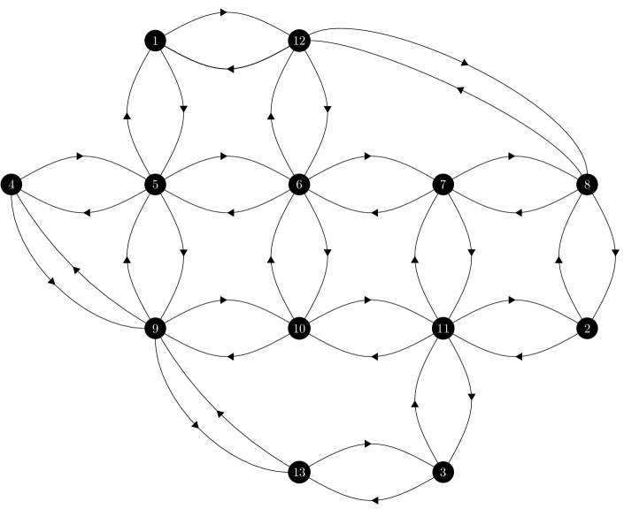
Figure 8: Nguyen-Dupuis network with 13 nodes and 38 links.

Example 5 (VMT Estimation)

We consider the Nguyen-Dupuis network  [38] of Fig. 8. For simplicity, assume all links have the same length but different paths have different lengths. There are 8 OD plausible pairs: $\{\text{\acs{OD} pair}~{}1-2,\text{\acs{OD} pair}~{}1-3,\text{\acs{OD} pair}~{}2-1,\text{\acs{OD} pair}~{}2-4,\text{\acs{OD} pair}~{}3-1,\text{\acs{OD} pair}~{}3-4,\text{\acs{OD} pair}~{}4-2,\text{\acs{OD} pair}~{}4-3\}$, with 50 alternative paths. To save space, we do not list these paths but refer the reader to [22]. We consider a set of $\boldsymbol{x}\in\mathbb{R}^{50}$ with 8 non-zero entries, so there is one true path for each OD pair. For each measurement we solve (17) and (18) and compute the recovery rate for different number of link measurements. We repeat this for 500 trials and consider recovery when $\|\widehat{\boldsymbol{x}}-\boldsymbol{x}\|_{2}\leq 0.001$, where $\widehat{\boldsymbol{x}}$ is the solution of (17) or (18). Fig. 9 shows the recovery results. Recovery improves with the number of measurements.

It is revealing to look at cases when exact recovery fails. Since a solution to (17) is a lower bound to the VMT, and a solution to  (18) is an upper bound, the ratios $\boldsymbol{v}^{T}\widehat{\boldsymbol{x}}_{\text{VMT Min}}/\boldsymbol{v}^{T}\boldsymbol{x}<1<\boldsymbol{v}^{T}\widehat{\boldsymbol{x}}_{\text{VMT Max}}/\boldsymbol{v}^{T}\boldsymbol{x}$ measure the accuracy of the estimates when recovery fails. ($\boldsymbol{v}^{T}$ is the transpose of the vector $\boldsymbol{v}=[v_{1},v_{2},\dots,v_{N}]^{T}$.) Fig.9 displays the mean values of the ratios when exact recovery fails as a function of the number of link measurements. With 22 measurements both (17) or (18) yield $80\%$ recovery. But even in the $20\%$ of the trials that exact recovery fails, the solutions are within 5 percent of the true value.

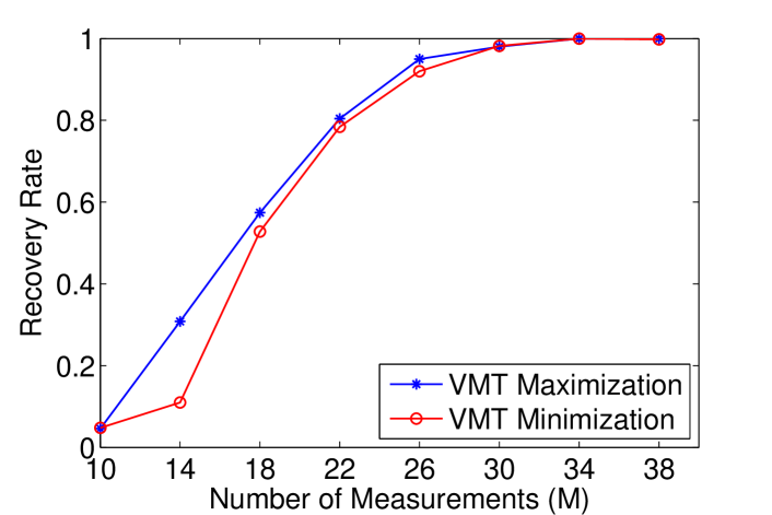
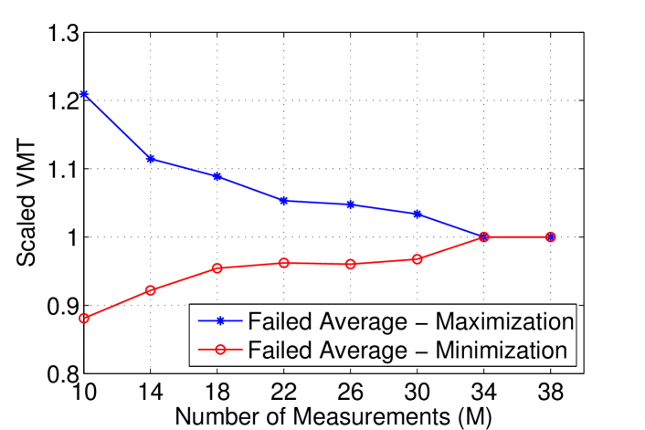
Figure 9: (Example 5) VMT estimation of Nguyen-Dupuis network. (a) Recovery results. For each measurement, we solve (17) and (18) and compute the recovery rate for different number of link measurements. We repeat this for 500 trials and consider recovery when $\|\sum v_{i}(\widehat{{x}}_{i}-{x}_{i})\|_{2}\leq 0.001$ where $\widehat{\boldsymbol{x}}$ is the recovered solution solving (17) or (18). (b) Mean value of $\boldsymbol{v}^{T}\widehat{\boldsymbol{x}}_{\text{VMT Min}}/\boldsymbol{v}^{T}\boldsymbol{x}$ and $\boldsymbol{v}^{T}\widehat{\boldsymbol{x}}_{\text{VMT Max}}/\boldsymbol{v}^{T}\boldsymbol{x}$ when (17) and (18) fail to exactly recover, respectively.

VII Case Study in East Providence

We apply CODE to traffic data recorded from an area in East Providence. Figure 10 depicts the map and the network of the area. The corresponding $A$ matrix has $10$ rows (number of measurements) and $33$ columns (number of paths). To save space we do not display $A$ and focus on the recovery results summarized in Fig. 11. The solution has only a few non-zero entries. The most significant path ($p_{10}$) is along the Grand Army of the Republic Highway ($\ell^{1}_{8}\to\ell^{8}_{9}$). This result further confirms that there usually exists a sparse path allocation which can be recovered using CODE.

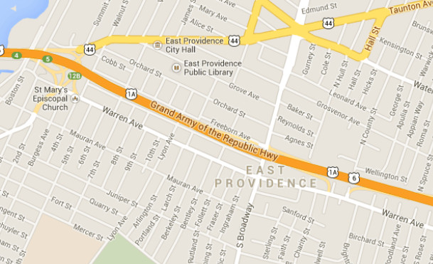
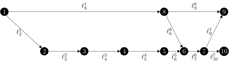
Figure 10: Case study of CODE on real data. (a) Map of the area under study in East Providence (Grand Army of the Republic Hwy and Warren Ave). (b) Schematic of the area under study. There are a total of 33 paths associated with OD pairs while 10 link flow measurements are available.

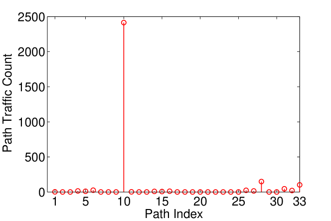
Figure 11: The recovered path allocation using CODE associated with the considered area in East Providence as shown in Fig. 10 and Fig. 10. As can be seen, the solution has only a few non-zero entries. The most significant path is the path on the Grand Army of the Republic Highway ($\ell^{1}_{8}\to\ell^{8}_{9}$).

VIII Conclusions and Future Work

We proposed CODE, an algorithm to estimate OD flows and their path allocations. Three variants of CODE (noiseless, noisy, and weighted) were considered, all involving $\ell_{1}$-minimization. Examples suggest that when the true path allocation is suitably sparse, CODE recovers the unknown variables exactly, even from a highly underdetermined set of linear equations.

Future directions for work include examining large networks to understand better the relation between sparsity, accuracy and computational effort. Also worth investigation is the incorporation of additional OD information obtained via Bluetooth or cell phone records. Another interesting question is to use CODE to determine path allocations that form a user equilibrium. Yet another direction concerns the selection of additional link counts that improve recovery.

Borhan M. Sanandaji is a postdoctoral scholar at the University or California, Berkeley in the Electrical Engineering and Computer Sciences department. He received his Ph.D. degree (2012) in electrical engineering from the Colorado School of Mines and his B.Sc. degree (2004) in electrical engineering from the Amirkabir University of Technology (Tehran, Iran). His current research interests include compressive sensing, low-dimensional modeling, and big physical data analytics with applications in energy systems, control, and transportation.

Pravin P. Varaiya is Professor of Graduate School in the Dept. of Electrical Engineering and Computer Sciences at the University of California, Berkeley. His current research concerns transportation networks and electric power systems. He received the Field Medal and Bode Prize of the IEEE Control Systems Society, the Richard E. Bellman Control Heritage Award, and the Outstanding Research Award of the IEEE Intelligent Transportation Systems Society. He is a Fellow of IEEE, a member of the National Academy of Engineering, and a Fellow of the American Academy of Arts.

References

- [1] H. J. Van Zuylen and L. G. Willumsen, “The most likely trip matrix estimated from traffic counts,” Transportation Research Part B: Methodological, vol. 14, no. 3, pp. 281–293, 1980.
- [2] E. Cascetta, “Estimation of trip matrices from traffic counts and survey data: a generalized least squares estimator,” Transportation Research Part B: Methodological, vol. 18, no. 4, pp. 289–299, 1984.
- [3] M. G. H. Bell, “The estimation of origin-destination matrices by constrained generalized least squares,” Transportation Research Part B: Methodological, vol. 25, no. 1, pp. 13–22, 1991.
- [4] H. Yang, T. Sasaki, Y. Iida, and Y. Asakura, “Estimation of origin-destination matrices from link traffic counts on congested networks,” Transportation Research Part B: Methodological, vol. 26, no. 6, pp. 417–434, 1992.
- [5] T. Abrahamsson, “Estimation of origin-destination matrices using traffic counts – A literature survey,” International Institute for Applied Systems Analysis - IIASA, vol. 27, p. 76, 1998, technical Interim Report IR-98-021.
- [6] M. L. Hazelton, “Some comments on origin-destination matrix estimation,” Transportation Research Part A: Policy and Practice, vol. 37, no. 10, pp. 811–822, 2003.
- [7] E. Bert, “Dynamic urban origin-destination matrix estimation methodology,” Ph.D. dissertation, EPFL, 2009.
- [8] S. Bera and K. V. Krishna Rao, “Estimation of origin-destination matrix from traffic counts: the state of the art,” European Transport, no. 49, pp. 3–23, 2011.
- [9] N. J. Van Der Zijpp, “Dynamic origin-destination matrix estimation from traffic counts and automated vehicle identification data,” Transportation Research Record: Journal of the Transportation Research Board, vol. 1607, no. 1, pp. 87–94, 1997.
- [10] Y. Asakura, E. Hato, and M. Kashiwadani, “Origin-destination matrices estimation model using automatic vehicle identification data and its application to the han-shin expressway network,” Transportation, vol. 27, no. 4, pp. 419–438, 2000.
- [11] J. Kwon and P. Varaiya, “Real-time estimation of origin-destination matrices with partial trajectories from electronic toll collection tag data,” Transportation Research Record: Journal of the Transportation Research Board, vol. 1923, no. 1, pp. 119–126, 2005.
- [12] X. Zhou and H. S. Mahmassani, “Dynamic origin-destination demand estimation using automatic vehicle identification data,” IEEE Transactions on Intelligent Transportation Systems, vol. 7, no. 1, pp. 105–114, 2006.
- [13] M. Bierlaire, “The total demand scale: a new measure of quality for static and dynamic origin–destination trip tables,” Transportation Research Part B: Methodological, vol. 36, no. 9, pp. 837–850, 2002.
- [14] J. Barceló and J. Casas, “Dynamic network simulation with AIMSUN,” in Simulation approaches in transportation analysis. Springer, 2005, pp. 57–98.
- [15] I. Okutani and Y. J. Stephanedes, “Dynamic prediction of traffic volume through kalman filtering theory,” Transportation Research Part B: Methodological, vol. 18, no. 1, pp. 1–11, 1984.
- [16] M. Cremer and H. Keller, “A new class of dynamic methods for the identification of origin-destination flows,” Transportation Research Part B: Methodological, vol. 21, no. 2, pp. 117–132, 1987.
- [17] X. Zhou, S. Erdogan, and H. S. Mahmassani, “Dynamic origin-destination trip demand estimation for subarea analysis,” Transportation Research Record: Journal of the Transportation Research Board, vol. 1964, no. 1, pp. 176–184, 2006.
- [18] İ. Ö. Verbas, H. S. Mahmassani, and K. Zhang, “Time-dependent origin-destination demand estimation,” Transportation Research Record: Journal of the Transportation Research Board, vol. 2263, no. 1, pp. 45–56, 2011.
- [19] D. L. Donoho, “Compressed sensing,” IEEE Transactions on Information Theory, vol. 52, no. 4, pp. 1289–1306, 2006.
- [20] E. J. Candès, “Compressive sampling,” in Proc. of the International Congress of Mathematicians, vol. 3, pp. 1433–1452, 2006.
- [21] E. J. Candès and M. Wakin, “An introduction to compressive sampling,” IEEE Signal Processing Magazine, vol. 25, no. 2, pp. 21–30, 2008.
- [22] E. Castillo, P. Jiménez, J. M. Menéndez, and A. J. Conejo, “The observability problem in traffic network models: Algebraic and topological methods,” Computer-Aided Civil and Infrastructure Engineering, vol. 23, no. 3, pp. 208–222, 2008.
- [23] E. J. Candès, J. Romberg, and T. Tao, “Robust uncertainty principles: Exact signal reconstruction from highly incomplete frequency information,” IEEE Transactions on information theory, vol. 52, no. 2, pp. 489–509, 2006.
- [24] S. S. Chen, D. L. Donoho, and M. A. Saunders, “Atomic decomposition by basis pursuit,” SIAM Journal on Scientific Computing, vol. 20, no. 1, pp. 33–61, 1999.
- [25] E. J. Candès and T. Tao, “Decoding via linear programming,” IEEE Transactions on Information Theory, vol. 51, no. 12, pp. 4203–4215, 2005.
- [26] H. Ohlsson, L. Ljung, and S. Boyd, “Segmentation of ARX-models using sum-of-norms regularization,” Automatica, vol. 46, no. 6, pp. 1107–1111, 2010.
- [27] R. Tth, B. M. Sanandaji, K. Poolla, and T. L. Vincent, “Compressive system identification in the linear time-invariant framework,” in Proc. th IEEE Conference on Decision and Control and European Control Conference, pp. 783–790, 2011.
- [28] B. M. Sanandaji, “Compressive system identification (CSI): Theory and applications of exploiting sparsity in the analysis of high-dimensional dynamical systems,” Ph.D. dissertation, Colorado School of Mines, 2012.
- [29] P. Shah, B. N. Bhaskar, G. Tang, and B. Recht, “Linear system identification via atomic norm regularization,” in Proc. th IEEE Conference on Decision and Control, pp. 6265–6270, 2012.
- [30] B. M. Sanandaji, T. L. Vincent, K. Poolla, and M. B. Wakin, “A tutorial on recovery conditions for compressive system identification of sparse channels,” in Proc. th IEEE Conference on Decision and Control, pp. 6277–6283, 2012.
- [31] B. M. Sanandaji, M. B. Wakin, and T. L. Vincent, “Observability with random observations,” to appear in IEEE Transactions on Automatic Control, 2013. [Online]. Available: arXiv:1211.4077
- [32] J. Zhao, N. Xi, L. Sun, and B. Song, “Stability analysis of non-vector space control via compressive feedbacks,” in Proc. th IEEE Conference on Decision and Control, pp. 5685–5690, 2012.
- [33] B. M. Sanandaji, T. L. Vincent, and M. B. Wakin, “Compressive topology identification of interconnected dynamic systems via clustered orthogonal matching pursuit,” in Proc. th IEEE Conference on Decision and Control, pp. 174–180, 2011.
- [34] W. Pan, Y. Yuan, J. Goncalves, and G. Stan, “Reconstruction of arbitrary biochemical reaction networks: A compressive sensing approach,” in Proc. th IEEE Conference on Decision and Control, pp. 2334–2339, 2012.
- [35] E. J. Candès, M. B. Wakin, and S. P. Boyd, “Enhancing sparsity by reweighted minimization,” Journal of Fourier analysis and applications, vol. 14, no. 5-6, pp. 877–905, 2008.
- [36] L. Hoang and V. P. Poteat, “Estimating vehicle miles of travel by using random sampling techniques,” Transportation Research Record, no. 779, 1980.
- [37] R. K. Kumapley and J. D. Fricker, “Review of methods for estimating vehicle miles traveled,” Transportation Research Record: Journal of the Transportation Research Board, vol. 1551, no. 1, pp. 59–66, 1996.
- [38] S. Nguyen and C. Dupuis, “An efficient method for computing traffic equilibria in networks with asymmetric transportation costs,” Transportation Science, vol. 18, no. 2, pp. 185–202, 1984.