Modeling ringdown: Beyond the fundamental quasinormal modes
Abstract
While black hole perturbation theory predicts a rich quasi-normal mode structure, technical challenges have limited the numerical study of excitations to the fundamental, lowest order modes caused by the coalescence of black holes. Here, we present a robust method to identify quasinormal mode excitations beyond the fundamentals within currently available numerical relativity waveforms. In applying this method to waveforms of 68 initially nonspinning black hole binaries, of mass-ratios 1:1 to 15:1, we find not only the fundamental quasinormal mode amplitudes, but also overtones, and evidence for second order quasinormal modes. We find that the mass-ratio dependence of quasinormal mode excitation is very well modeled by a post-Newtonian-like sum in symmetric mass-ratio. Concurrently, we find that the mass-ratio dependence of some quasinormal mode excitations is qualitatively different from their post-Newtonian inspired counterparts, suggesting that the imprints of nonlinear merger are more evident in some modes than in others. We present new fitting formulas for the related quasinormal mode excitations, as well as for remnant black hole spin and mass. We also discuss the relevance of our results in terms of gravitational wave detection and characterization.
I Introduction
As we approach the era of gravitational wave (GW) detection, there is a tremendous effort to understand and predict the rich gravitational wave signals coming from all expected sources of radiation. These predictions are used to construct GW templates that will enable not only the recognition of GW signals within noise, but also the extraction of information about the source. It is for these purposes that the development of templates that include the final moments of binary black hole (BBH) coalescence is important for future GW detection.
While source populations remain uncertain, BBH systems are expected to account for multiple signals per year and, if systems with a total mass of a few hundred times that of our sun or larger are observed, detectors such as Advanced LIGO and the Einstein Telescope are most sensitive to the final stages of BBH coalescence Abadie:2010cf ; Belczynski:2010tb ; Mishra:2010tp ; Ajith:2009fz . In these final moments the two black holes (BHs) merge into a perturbed, remnant BH, whose gravitational radiation rings down like a struck bell. Very roughly put, if one were to observe the remnant at an orientation relative to its spin axis, and at a distance away, then the observable time domain strain of this decaying ringdown radiation may be written as the real part of
| (1) | ||||
Here, and are the real valued plus and cross polarization states. In general, a linear combination of these states will be detected Alcubierre.0707.4654 ; 2014arXiv1410.8310T .
If provided the remnant BH’s mass and spin, then the perturbation theory of isolated Kerr BHs informs us of Eq.(1)’s spatial multipoles and temporal frequencies: the Quasi-Normal Modes (QNMs) that dominate ringdown PreTeu73_2 ; leaver85 ; PhysRevD76Berti . However, in order to model astrophysically relevant ringdown signals the output of numerical relativity (NR) simulation is generally needed to tell us how much each multipolar component is excited for a given initial binary PhysRevD76Berti ; Kamaretsos:2011um .
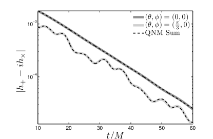
For this reason, applying BH perturbation theory to the analysis of NR ringdown has assisted in the creation of inspiral-merger-ringdown templates Taracchini:2013rva ; Damour:2009kr ; Pan:2009wj , and revealed novel relationships between the initial binary’s configuration and the remnant BH’s parameters Kamaretsos:2011um . But thus far, technical challenges have limited analysis primarily to the fundamental (lowest overtone) QNMs, while it has also been acknowledged that a more detailed application of perturbation theory to NR ringdown may be needed Kamaretsos:2011um ; Taracchini:2013rva ; Kelly:2012nd ; Dorband:2006gg ; Okuzumi:2008ej ; Schnittman:2007ij ; Buonanno:2006ui . As an example of ringdown’s potential complexity, Fig. 1 shows the time domain strain envelope of a potential 2:1 mass-ratio ringdown signal of an initially nonspinning BH binary, observed at two different lines of sight. Here we see that the sum of many QNMs precisely models NR ringdown data. This example case demonstrates that both the intrinsic QNMs of perturbation theory and the observer’s extrinsic line of sight contribute to the richness of possible ringdown signals.
In this study we assist in clarifying the extent to which QNMs beyond the fundamentals are pertinent to the physics and modeling of NR ringdown (e.g. Fig. 1). We consider the ringdown of 68 initially nonspinning BBH simulations of mass-ratios between 1:1 and 1:15. In doing so, we find that QNM excitation is exceptionally well modeled by a post-Newtonian-like (PN-like) expansion (Sec.IV). However, we also find that the excitation amplitudes of some QNMs differ qualitatively from their post-Newtonian (PN) counterparts, suggesting that the imprints of nonlinear merger are more evident in these QNMs than in others (Sec.VI.1). But first, we present a robust method to estimate multiple QNMs within NR ringdown (Sec.III.1). We then apply this method to a series of initially nonspinning NR runs of varying mass-ratio (Sec.III.2-IV.2). Lastly, we consider the results of our analysis (overtones and second order modes) in the context of ringdown-only templates (Sec.VI.2). Generally, our results may be of use for the construction of merger-ringdown templates.
A complete paper outline is given in Sec. I.3. A full summary of fitting formulas and coefficients for QNM excitations is given in Appendix A. For convenience, fits for the most dominant QNM excitation amplitudes in Eq.(1) are below:
| (2) | ||||
| (3) | ||||
| (4) | ||||
| (5) | ||||
| (6) | ||||
| (7) | ||||
| (8) | ||||
| (9) | ||||
| (10) |
Here, is the sum of the initial BH masses,
and is the symmetric mass-ratio,
The amplitudes are scaled relative to 10 after the peak luminosity in (Sec. I.2),
Note that the QNM frequencies, , are complex, and depend on the remnant BH’s parameters: spin magnitude and mass.
| (11) |
In Eq.(11), is the QNM’s central oscillation frequency, and the mode’s decay time. Each frequency may be conveniently computed using the mapping between and remnant BH parameters given in Eqs. 55 and 54, or Ref. Healy:2014yta , along with the phenomenological fitting formulas111Note that here are in units of while Berti:2005ys reports the unitless . for QNM frequencies in Ref. Berti:2005ys .
I.1 From QNMs and templates to NR ringdown analysis
Shortly after Vishveshwara’s 1970 discovery that perturbed black holes dissipate energy via gravitational ringdown, the study of perturbed BHs began a proliferation that now enables the creation of GW ringdown templates Vishv:1970 ; Berti:2009kk ; Caudill:2011kv . In 1971 Teukolsky and Press revealed that ringdown should be well approximated by a sum of eigenfunctions of Teukolsky’s master equation which describes first order departures from the Kerr metric Teu73_1 ; PreTeu73_2 ; LivRevQNM . For a BH of mass and dimensionless spin parameter,
these eigenfunctions are uniquely determined. Here is the magnitude of the final BH spin vector. Press later referred to Teukolsky’s set of radial, angular, and temporal eigenfunctions as QNMs LivRevQNM ; Berti:2009kk [Eq.(14)]. QNMs are multipoles with the usual polar and azimuthal indices, and . In addition, in loose analogy with acoustic theory, they are also labeled by an overtone number, , where, as increases, so does the typical QNM decay rate leaver85 . The QNMs are traditionally referred to as the fundamental modes.
Given that astrophysical BHs are expected to be described by only mass and spin, the work of developing GW templates that include ringdown is largely equivalent to modeling the excitations of Kerr QNMs for different progenitor binaries Caudill:2011kv ; Berti:2007zu . This work has largely focused on the most slowly decaying, fundamental QNMs, which correspond to first order departures from the Kerr metric.
However, it has been suggested that second order QNMs, resulting from nonlinear self-coupling of their first order counterparts, may also be pertinent Campanelli:1998jv ; Okuzumi:2008ej ; Nakano:2007cj ; Ioka:2007ak ; Pazos:2010xf ; Zlochower:2003yh . Although these second order QNMs have largely been studied for Schwarzschild BHs, where Regge-Wheeler-Zerilli techniques can be directly applied, formal results for the Kerr case do not appear to exceed Campanelli:1998jv , wherein the second order contribution’s wave equation is derived within the Newman-Penrose formalism.
This result demonstrates that the second order wave equation for Kerr, like its Schwarzschild counterpart, is sourced by a quadratic function of the first order modes. For this reason it is expected that the second order QNMs for Kerr are characteristically similar to those for Schwarzschild Ioka:2007ak . In particular, one might expect to find within Fig. 1 damped sinusoids whose frequencies and decay rates are sums of those from two first order modes222This is analogous to the anharmonic oscillator, in which the second order oscillation frequency is twice the first order one Ioka:2007ak ..
From these considerations it is clear that perturbation theory allows for an extremely rich space of possible ringdown signals. But given that the fundamental modes are the slowest damped, it is not immediately clear that modes beyond the fundamentals are pertinent to modeling of NR ringdown. Indeed, the single and two-mode ringdown-only templates of Ref. Caudill:2011kv only consider fundamental QNMs. Similarly, studies that focus on linking QNM excitation with initial binary parameters typically focus only on the fundamental modes Kamaretsos:2011aa ; Kamaretsos:2011um ; Kamaretsos:2012bs and, while work on templates that include both merger and ringdown has found that overtones are required to blend the two regions, a systematic study of overtone excitement is lacking Pan:2009wj ; Schnittman:2007ij ; Taracchini:2013rva ; Buonanno:2006ui . Moreover, there has been no work published on the detection of nonlinear second order QNMs within NR BBH coalescence. Here, we inform these areas by describing QNM excitation for a series of initially nonspinning, unequal mass BBH systems.
For the recovery of these initial parameters precise agreement between template and signal is needed. Concurrently, only qualitative agreement is needed for detection purposes Caudill:2011kv ; Berti:2007zu . Although a full exploration of detection and parameter estimation is beyond the scope of the current study, we note that the richness of possible signals depends not only on the configuration of the initial binary, but also the orientation of the BH’s final spin vector with respect to the observer’s line of sight.
As an example, consider again Fig. 1. Here we see that if this idealized signal is observed along the remnant BH’s final spin axis, , then the envelope of its time domain behavior appears to be dominated by a single exponentially decaying function, or equivalently, a single QNM; however, if observed at a significant angle with respect to the final spin axis, here , then many QNMs may visibly contribute. In order to model the complexities of these potential signals, we utilize the intersections between perturbation theory and NR.
I.2 Numerical relativity meets perturbation theory
NR waveforms are typically decomposed333 This decomposition is typically done such that the origin is at the initial binary’s center of mass. In general, this is not the location of the remnant BH if there is a nonzero recoil velocity. However, for the systems studied here, the typical distance traveled postmerger, is sufficiently small compared to the waveform extraction radius, making this initial center of mass location a good approximation for the position of the remnant BH. Nevertheless, as discussed in Sec. V , this does potentially introduce detailed effects that may not be inherent to the ringdown regime. into spin weighted-2 spherical harmonics, , such that the Weyl scalar is given by
| (12) |
For gravitational radiation, the orthogonality of these harmonics in both and ensures that this is a true spectral decomposition:
| (13) |
Here is the complex conjugate of , and we will focus on , the spherical harmonic multipoles of the Weyl scalar . The Weyl scalar is related to the observable strain via two time derivatives, Alcubierre.0707.4654 .
During ringdown, this choice of multipolar decomposition effectively casts the radiation as that corresponding to a perturbed nonspinning BH Alcubierre.0707.4654 . However the remnant of a BBH merger is typically a spinning BH.
For these cases, the perturbation theory of Kerr BHs Leaver:1986gd yields
| (14) | |||
| (15) |
where is the complex QNM frequency, are the spin weighted spheroidal harmonics, and are the complex QNM amplitudes or excitation coefficients whose magnitude is contingent on where is chosen to be zero Berti:2009kk ; PhysRevD.73.024013 ; Zhang:2013ksa .
For example, if is the time relative to the peak luminosity of , and one considers ringdown to include after , then Kamaretsos:2012bs . Here we consider to be in units of the initial binary mass, , which is canonically set to unity.
Generally, Eq.(14) is not an equality as power-law tails, of the form , are also expected in the postmerger regime Price:1972pw ; Leaver:1986gd . While, in principle, these power-law contributions may be significant near the radiation’s peak, a host of numerical studies has shown them to be extremely weak throughout the subsequent QNM regime444 In contrast to the current study, which evolves the full Einstein equations, studies that are able to resolve late-time power-law decay evolve Teukolsy’s equation (e.g. KrivanLaguna96 ), which is motivated by first-order departures from the Kerr space-time PhysRevLett.29.1114 . Leaver:1986gd ; PhysRevD76Berti . In particular, while all power-law functions decay slower than exponentials, they also require excitation coefficients much larger than those of QNMs to contribute significantly to the waveform. Therefore there is a heuristic expectation that the power-law tails eventually dominate the postmerger waveform, but only at very late times Mitsou:2010jv ; Scheel:2003vs ; Leaver:1986gd ; Harms:2013ib . Indeed, recent NR codes that focus on binary black hole coalescence (BBC) have empirically verified this expectation Schnittman:2007ij ; PhysRevD76Berti ; Buonanno:2006ui ; Kamaretsos:2012bs . Numerical studies that focus specifically on solving Teukolsky’s equation do find that power-law tails are physically meaningful, but only at late times, and at amplitudes that are very likely inaccessible to codes that solve Einstein’s equations in full KrivanLaguna96 ; Harms:2013ib .
While the current study, in part, seeks to describe ringdown in unprecedented detail, we also find that for the systems considered, power-law decay can be neglected.555This is readily visible in Fig. 3’s lower panel where, if power-law tails did contribute significantly, they would cause a localized feature near zero frequency.
For simplicity we have written Eq.(14) as a sum over the first order QNM indices only. If written explicitly, the second order QNM terms, being proportional to products of two first order QNMs, would be labeled by six indices, Okuzumi:2008ej ; Nakano:2007cj ; Ioka:2007ak . We have also neglected to explicitly write the conjugate or mirror-mode terms which arise from Teukolsky’s azimuthal equation having two linearly independent solutions that, due to nonzero BH spin, are not the complex conjugates of each other leaver85 ; Berti:2005ys .
An additional consequence of nonzero BH spin is that the spheroidal harmonics, while orthogonal in , are not orthogonal in for the complex QNM frequencies of ringdown666 Specifically, we are concerned with spheroidal harmonics with complex frequency and of spin weight , which correspond to exponentially damped time-domain waveforms.PhysRevD.73.024013 ; Stewart:1975vg , making a spectral decomposition of the form of Eq.(13) not possible. However, just as the Kerr metric reduces to the Schwarzschild metric for nonspinning BHs, so do the spheroidal harmonics reduce to the sphericals. Substituting Eq.(14) into Eq.(13) illustrates this point by revealing that the spherical multipoles of NR are each a sum of many spheroidal QNMs where, in the limit, only the term survives
| (16) | |||
| (17) |
This was first noted in 1973 by Press and Teukolsky PreTeu73_2 who used standard operator perturbation theory to show that
| (18) |
Here are related to the Clebsch-Gordon coefficients Berti:2005ys ; Teu73_1 .
Equations 16 through I.2 motivate two approaches to characterize QNM excitations, : single-mode and multimode fitting.
Single-mode fitting.—
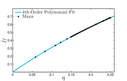
The first category makes the practical assumption that Eq.(16) is dominated by the term, and thereby estimates the QNM amplitudes by fitting a single mode to . Although this single-mode approach has been shown to be effective for the first few multipoles Kamaretsos:2011aa ; PhysRevD76Berti , in principle, it neglects the presence of overtones and BH spin Berti:2009kk ; Kelly:2012nd . Moreover, because Eq.(I.2) says that the mixing between spherical and spheroidal harmonics becomes more prevalent for higher spins, we may hypothesize that single-mode fitting incurs residuals that are qualitatively proportional to the remnant BH’s spin. In particular, Fig. 2 shows that initially nonspinning, quasicircular BBH systems coalesce to form a remnant BHs whose final spin is proportional to the initial binary’s symmetric mass-ratio. We would therefore expect single-mode fitting of these systems to perform better for low mass-ratios (), and worse at higher mass-ratios ().
Specifically, while it has been shown that Eq.(17)’s can be on the order of 0.10 for moderate values of PhysRevD.73.024013 , Eq.(16) communicates that the relative values of different ultimately determine the significance of each QNM term Kelly:2012nd .
Multimode fitting.—
The second category attempts to fit each term in Eqn. (16), and therefore requires the simultaneous fitting of multiple QNMs within each spherical multipole. Although this multimode approach is more faithful to the fact that the BHs of interest are spinning, current fitting methods have had limited success Buonanno:2006ui ; Berti:2007dg ; gr-qc/0608091 . The difficulty is primarily due to complexity: within each , a multimode fitting algorithm must optimize over as well as the total number of significant QNMs, . There are secondary difficulties arising from data accuracy and numerical artifacts. As a result, the multimode approach is a dimensional optimization problem of combinatoric complexity whose solution must be robust against numerical errors. It is a lot like trying to identify a musical chord by ear.
I.3 Structure of the paper
In the current study we present a multimode fitting method, and apply it to the NR ringdown of 68 initially nonspinning, unequal mass-ratio binaries with symmetric mass-ratios between and .
We report estimates for the QNM excitations of not only fundamental modes, but also for overtones and what appear to be second order modes. We go on to discuss our results in the context of phenomenological ringdown models and future detection scenarios. First, in Sec. II.1 we review the single-mode approach, and report fit residuals. As described in Sec. II.2, for nominal fitting regions, we find that single-mode fitting incurs roughly fitting errors for the best case scenario, and greater error in the worst case scenarios. We also review the systemic dependence of residuals with final BH spin. In Sec. III.1 we introduce our multimode fitting method, and compare it with other approaches using mock data in noise, then review found QNM amplitudes and residual errors. In Sec. IV, we present post-Newtonian inspired fits to the dominant QNM excitations across the range of mass-ratios. In Sec. V we discuss the limitations of our results, and their consistency with perturbation theory. Finally, in Sec. VI, we discuss our results in the contexts of analytic (nonlinear) perturbation theory, and review the significance of our findings to a mock detection scenario.
II Motivations for multimode Fitting
 |
|
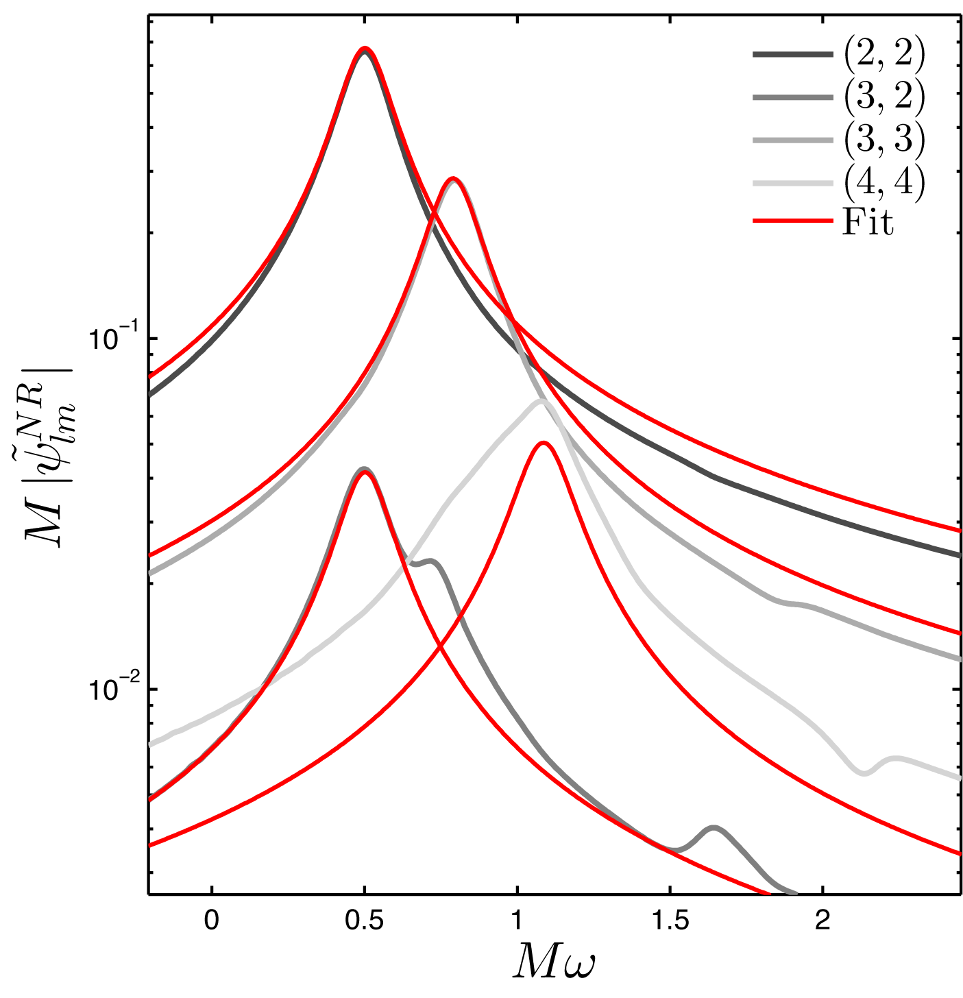
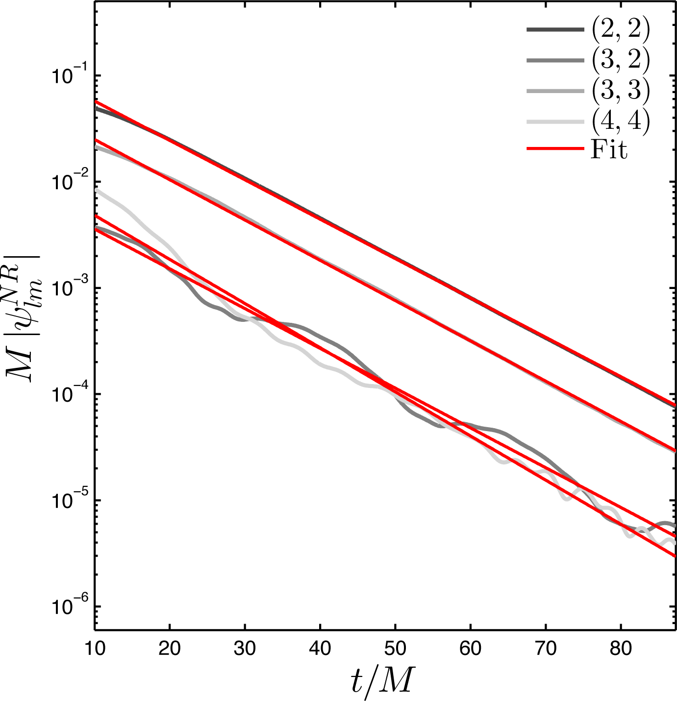
Let us first consider the single-mode fitting approach discussed in Sec. I.2. Figure 3 shows single-mode fits for a 2:1 mass-ratio binary. While we can see that in this case the subdominant are not all simple functions, the dominant multipoles do appear to have exponentially decaying envelopes, and so are well modeled by a single QNM. Indeed, previous studies have found success in treating the dominant multipoles as single QNMs during ringdown Kamaretsos:2011aa ; PhysRevD76Berti . In particular, this approach has led to effective numerical estimates of BH final spin and mass, as well as the characterizations of fundamental QNM amplitudes with mass-ratio, and initial spin magnitude Hannam:2010ec ; Kamaretsos:2012bs . It is therefore fair to suppose that more detailed QNM information is not needed in order to capture ringdown’s dominant physics. In what follows, we test this heurism by first outlining the single-mode approach, and then investigating the dependence of fit residuals with initial binary parameters (Fig. 4).
II.1 Single-mode fits
First, we outline a qualitatively general single-mode fitting procedure to estimate the fundamental () QNM excitations:
-
a.
Given the set of , we define ringdown to be the region relative to the peak luminosity777 As will be discussed in Sec. III.1, we consider multiple fitting regions in order to characterize both the data and fit. In the case of single-mode fitting, fitting regions were chosen to encompass between 86 and 74 . For the multimode fitting approach to be discussed in Sec. III.1, each waveform was windowed and padded after the onset of numerical noise to maintain a consistent frequency domain resolution. of Kamaretsos:2011aa .
-
b.
To calculate the waveform’s phase, , and envelope, , we then consider the standard representation for the fit:
-
c.
We then use linear least-squares fitting to model and as lines in the time domain:
(19) (20) where is the complex phase of .
-
d.
Upon calculating the fit parameters, , we calculate the fractional root-mean-square error,
(21) Here is typically much less than for good fits, and of order or greater for poor fits. More carefully, as discussed in Sec.II.3, is susceptible to being biased by numerical noise. In the worst case scenario, where noise dominates the data to be fit, may correspond to a minimum residual with respect to fit parameters.
Typical single-mode fits are shown in Fig. 3 for a mass-ratio binary, with the fitting region starting after the peak luminosity in . Here, as well as throughout this paper, the Fourier transform of waveforms, , will be denoted as . Note that the multipoles are well fit, with associated errors . However, a notable exception is the multipole with and order of magnitude higher at .
Moreover, as has been found in previous studies, we also find that the multipoles are generally not well fit by a single QNM. For example, the multipole, , is known to have a significant contribution from the term in Eq.(16) Kelly:2012nd ; Buonanno:2006ui ; PhysRevD76Berti ; 0707.0301 . This may be recognized in the lower panel of Fig. 3, where is seen have its dominant peak not at ’s central frequency888The central frequency is given by the real part of the QNM frequency. of , but at , directly under the peak of .
In what follows we discuss the residual error of the single-mode approach. In particular, we ask if the errors are dominated by numerical artifacts (e.g. resolution related errors Hannam:2010ec ), or if the errors are dominated by the effects of nonzero BH spin.
II.2 Single-mode fits: Results and residuals
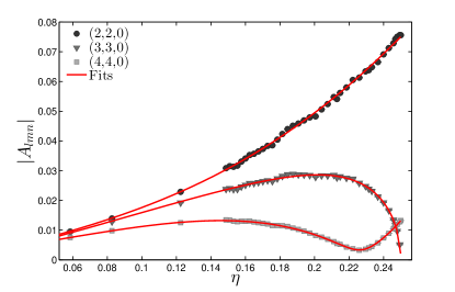
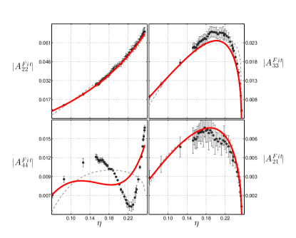
To investigate the residuals incurred by single-mode fitting, we consider 36 initially nonspinning, unequal mass binaries with between and . The left panel of Fig. 4 shows typical fit excitation amplitudes, , and the right panel shows the corresponding residual errors (Eq.(21)). The left panel of Fig. 4 shows that QNM excitation appears regular with symmetric mass-ratio with the mode dominating. The fitting model proposed in Ref. Kamaretsos:2011aa is also plotted. The lower left panel of Fig. 4 indicates that the has a significant local minimum at () for the resolution in considered here. The QNM has been found to exhibit a similar local minimum Kelly:2012nd .
Turning to the right panel of Fig. 4, the and cases show monotonically decreasing trends. This trend may be due to the difference between spherical and spheroidal harmonics, which is proportional to final BH spin [Eq.(I.2)], and is therefore also proportional to symmetric mass-ratio (Fig. 2); thus, single-mode fitting may incur systematic errors that decrease with .
While the and estimates display a more complicated behavior, their overall decrease with suggests that these cases may be significantly affected not only by QNMs beyond the fundamentals, but also by other sources of errors.
II.3 Sources of error
 |
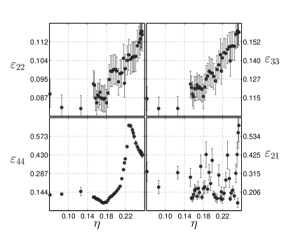 |
To contrast how much of each is attributed to nonfundamental QNMs rather than other factors, we briefly review the primary numerical sources of error: finite resolution and extraction radius. In aggregate, we find that the overall effect of these errors contributes to a noise floor that, at , is typically 2 orders of magnitude lower than the relative fit errors shown in the right panel of Fig. 4. As a general consequence, is increasingly biased by numerical noise as approaches the noise floor. This is most evident for , which displays a pronounced increase as sweeps through its local minimum.
For the waveforms used here, the simulation grid is structured so that there is a central grid of maximal resolution within peripheral grids whose resolution decreases by a factor of 2 at each outward extension. The result is an inherent tension between the finite extraction radius, and the finest grid resolution (see Sec. V.3 for an expanded discussion of finite extraction radius and related gauge effects.). In effect, this means that up to are resolved spatially, with points oscillation cycle, and temporally with points per cycle999 These figures were calculated using the QNM frequency for an equal mass nonspinning BBC. In the same case, we find that there are points temporally and points spatially within the typical amplitude decay rate. Because QNM frequency decreases as final spin decreases, these numbers increase as the initial binary becomes more unequal (e.g. Fig. 2).. In particular, we find that duplication of Fig. 4 at is consistent with resolutions {0.62,1.125,1.25} times that of the values quoted above, and, therefore, the right panel of Fig. 4 is not dominated by resolution effects.
Our post-merger data contain low amplitude, high frequency oscillations that contribute at most 5% to our estimates of residual error, , and appear to be an effect of discretization. This high frequency contribution is visible in Fig. 3 as low amplitude features to the right of each central frequency. While the high frequency of these oscillations means that their contribution to the mean residual difference is small, the magnitude of these oscillations is also marginal across multipoles, and appears at comparable power at the same positive and negative frequency. As seen in Fig. 3, this frequency varies from multipole to multipole. Despite their pervasiveness, these features are too high to be pertinent QNM frequencies [Eq. 17], and are likely artifacts due to our simulation’s containing nonzero power at frequencies beyond the resolvable limit. Comparison with public NINJA waveforms Ajith:2012az reveals that these features show up inconsistently across NR implementations, which suggests that they are both spurious effects due to discretization, and independent of the dominant physics at play101010 Importantly, as will be discussed in Sec. III.1, they are also well localized in the frequency domain, which allows us to effectively filter them out during multimode fitting..
As a result, we conclude that the fit errors in Fig. 4 are not dominated by numerical artifacts, but instead primarily due to choice of representation: the spherical representation of Eq.(12), versus the spheroidal representation of Eq.(14). Kelly et al recently came to a similar conclusion by considering only the spherical multipole.
III Multimode Fitting: From Spherical to Spheroidal
As discussed in the previous section, the single-mode fitting of spherical multipoles, , results in relatively significant residual errors (greater than 5%) that are systematic in final BH spin. This spin-systematic behavior verifies the hypothesis encapsulated by Eq.(16): NR ringdown is not a single QNM, but a sum of QNMs. We are therefore motivated to pursue a multimode fitting approach to describe QNM excitations for different mass-ratios. In particular, we will seek to extract spheroidal information from the spherical harmonic multipoles of NR waveforms.
By noting that the general fitting problem is multilinear in the set of decaying sinusoids given by perturbation theory [Eq.(16)], we present a method based upon ordinary linear least-squares fitting (OLS) to estimate spheroidal QNM amplitudes within each spherical multipole. We find that this particular choice of fitting routine (e.g. the least-squares approach used here) is not as important as its surrounding algorithm which aims to significantly reduce the problem’s complexity. This is, in part, accomplished by utilizing a standard greedy algorithm in addition to OLS fitting. We refer to our approach as the greedy-OLS method.
For reference, we test our method with artificial data within artificial numerical noise to present a brief comparison between our greedy-OLS method and the modified Prony method Berti:2007dg ; Osborne95amodified in Sec.III.2. We then present estimates of the QNM excitations due to initially nonspinning BH binaries of variable mass ratio.
III.1 Multimode fitting method
We have developed and implemented the following fitting procedure to estimate QNM amplitudes:
-
a.
Given the set of , we define ringdown to be the region relative to the peak luminosity of Kamaretsos:2011um . Because the following procedure involves taking the discrete Fourier transform, each ringdown waveform is appropriately windowed at the noise floor, and padded to ensure consistent frequency domain resolution.
-
b.
Following Eq.(16), we assert that NR ringdown, , may be well approximated by sum of QNMs. As our numerical waveforms are of limited accuracy, we consider this sum to be finite:
(22) where
(23) and
(24) While Eq.(22)’s is the estimate QNM amplitude, for notational simplicity we will henceforth refer to it as . Moreover, the above summation is only over , as is fixed by Eq.(16).
Here, the apparent horizon may be used to estimate the BH’s final mass and spin, and Frauendiener:2011zz . Alternatively, one may estimate the final BH mass and spin by optimizing the multimode fit of a single , as each QNM frequency is determined by and (Appendix C). Specifically, the dependence of the QNM frequencies on and may be utilized by either direct calculation (e.g. leaver85 ), as used here, or by phenomenological fit (e.g. Berti:2005ys )111111We find these two approaches to nominally agree to within 1% of each other (Appendix C). .
-
c.
In the language of least-squares fitting, we seek to cast Eq.(22) in the form of a set of normal equations:
(25) or equivalently,
(26) To do so, we choose to make the following series of definitions:
(27) (28) (29) where and is an complex valued matrix. The consistency of Eqs. (27)-(29) with Eq.(25) is evident upon plugging Eq.(22) into Eq.(28).
If is nonsingular, then the complex fitting amplitudes are given by
(30) Recalling that Eq.(27) defines in terms of the complex QNM amplitudes, we equivalently have that estimates for the spheroidal coefficients in Eq.(22) are given by the th element of
In effect, Eqs. (27)-(29) entail taking the Fourier transform of the ringdown waveform, and performing semianalytic, linear least-squares fitting in the basis of damped sinusoids allowed by perturbation theory.
This approach imposes that be composed of the QNM frequencies of perturbation theory rather than treating them as fitting parameters, and therefore, the total dimensionality of the fitting problem is reduced from to : . However, since Eq.(30) allows for the simultaneous determination of ’s real and imaginary parts, the problem has effectively been reduced to dimensions. But note that the problem is not truly linear in , as the fit must be optimized over all likely combinations of QNMs allowed by perturbation theory [Eq.(16)].
-
d.
To manage this last optimization, we first limit the set of allowed QNMs to those whose is above [Eq.(17)]. This choice is practically equivalent to only allowing to differ from by at most 2, and simultaneously limits the largest allowed fitting frequency to be well below that of the non-QNM features discussed in Sec. II.3. We then use a greedy 121212Our greedy algorithm builds a list of QNMs by starting with , and adding only QNMs to that reduce the fit error (Eq.(21)). This process continues iteratively until the addition of at most two QNMs does not better the fit significantly, or causes the fit to become worse. A broader description of greedy algorithms may be found in Cormen2001introduction . algorithm to estimate the optimal set of QNMs for each . We choose to guide the greedy process by using Eq.(21) averaged over different overlapping fitting regions 131313In particular, we average over 15 fitting regions whose starting time is equally spaced between and . Each is calculated by evaluating Eq.(30) and Eq.(21) on the sub-region..
-
e.
Once the optimal set of QNMs has been found, we estimate the spheroidal QNM amplitudes from Eq. 27),
(31) -
f.
To quantify the effect141414Please see Sec. V.1 for a somewhat expanded discussion. of on , we perform the above process for and then rescale each using the corresponding QNM decay rate such that is relative to . The resulting set, , describes how much each recovered agrees with our assumption that the choice of fitting regions corresponds to QNM dominated ringdown. For example, in the ideal case, where the fitting region contains only QNMs, every element would have the same value.
Throughout this paper, we describe the fitting region dependence of our results using error bars of width , where . In Fig. 4, a scaling factor of is used. Error bars for nonamplitude quantities have been calculated in a similar fashion. We choose to represent the error bars according to the range of values because the data of interest are inherently systematic, not random (Appendix B).
Now, for reference, we proceed by touching base with an alternative multimode approach of interest Berti:2007dg ; 0264-9381-28-8-085023 , the modified Prony method Osborne95amodified .
III.2 Multimode fits
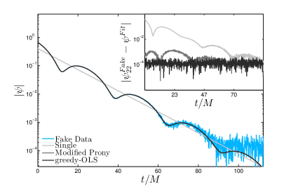
Before using the greedy-OLS algorithm developed in the preceding Sec., we compare it with a popular method for recovering damped sinusoids within noise that linearizes the fitting problem by framing each QNM as the root of a complex polynomial. If the number of data points is greater than the number of modes, this approach is called the modified Prony algorithm Osborne95amodified ; Berti:2007dg . In this Sec. we consider test data to demonstrate what we find to be the typical advantages of approaches like the the greedy-OLS algorithm. In particular, we ask: given fake data, , of known QNM composition, which algorithm returns the input QNMs and achieves the best fit?
| Method | Recovered QNMs | |
|---|---|---|
| Single (Sec.II.1) | (2,2,0) | |
| Modified PronyOsborne95amodified ; Smyth:2003 | (2,2,0),(3,2,0) | |
| Greedy-OLS (Sec.III.1) | (2,2,0),(3,2,0),(2,2,1) |
To portray a typical answer to this question, we construct to be composed of the QNMs with the addition of Gaussian noiseBerti:2007dg that is times smaller than the largest component amplitude. As the modified Prony algorithm treats QNM frequency and decay time as free parameters, we label each output frequency by its nearest QNM frequency.
Figure 5 compares the output of the greedy-OLS method to the results of the modified Prony algorithm Osborne95amodified and the single-mode fitting algorithm described in Sec.II.1. Table 1 lists the recovered QNMs and corresponding residual errors (Eq.(21)). While both the modified Prony and greedy-OLS methods produce qualitatively precise fits, the inset of Fig. 5 shows that the Prony method incurs a noticeably higher residual error. Turning to Table 1, we see that this larger residual error corresponds to the Prony method’s not capturing the overtone. This missing mode illuminates two related disadvantages of Prony methods when applied to QNM analysis:
-
a.
The treatment of QNM frequency (Eq.(11)) as a free parameter increases the difficulty in assigning output frequencies to those predicted by perturbation theory.
-
b.
The method’s output frequencies are susceptible to spurious deviations from the structure predicted by BH perturbation theory. This aspect of the algorithm complicates the process of estimating BH final mass and spin Berti:2005ys .
For these reasons, throughout the sections that follow, we favor the greedy-OLS algorithm. However, we must also note that any fitting algorithm that uses prior information from perturbation theory to perform multimode fitting may be just as effective. For example, we find that using the Levenberg-Marquardt algorithmmarquardt:1963 , in place of Eq.(30), is just as potent at estimating the QNM terms in Eq.(22), but only if fitting frequencies are limited to those predicted by perturbation theory.
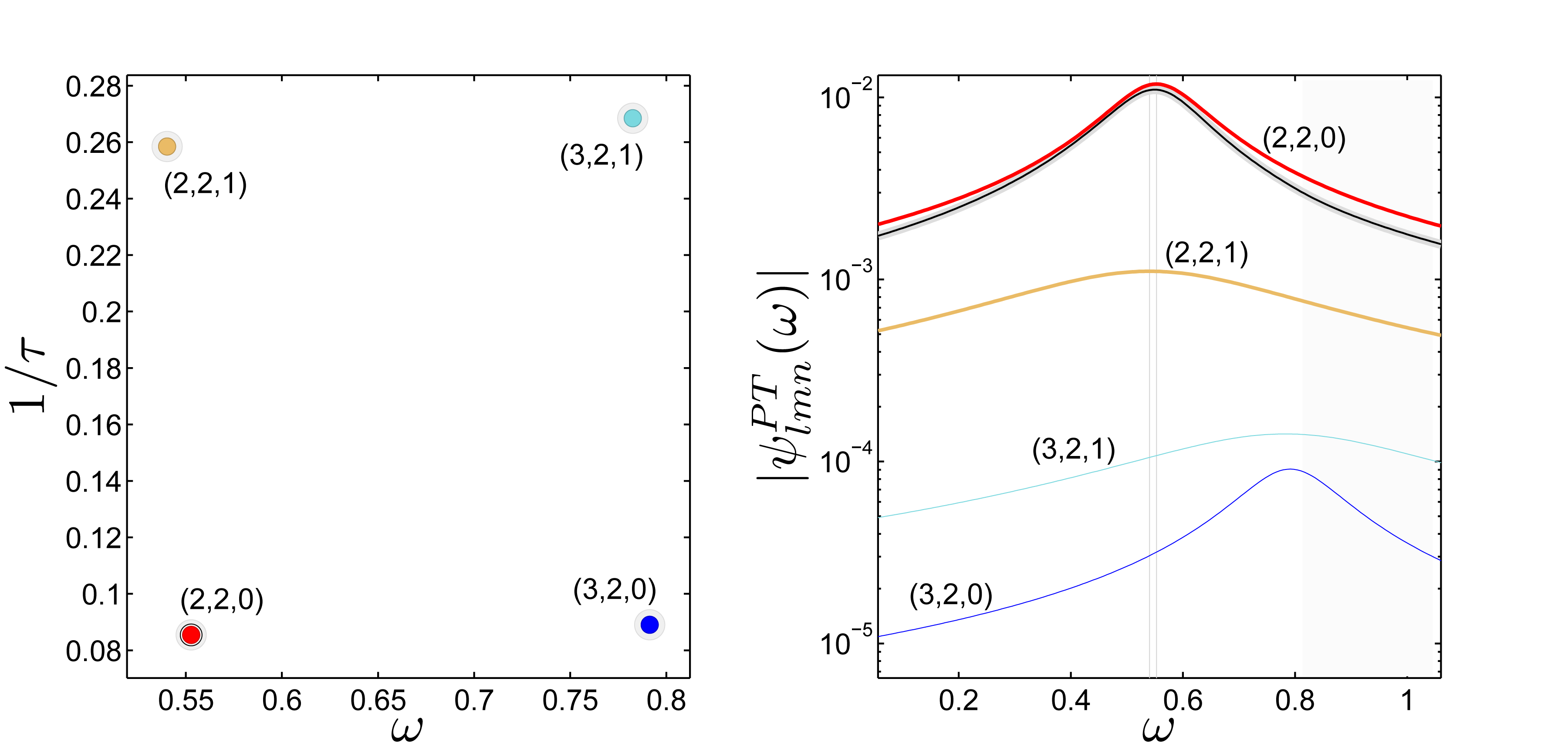
Now, with some confidence in the greedy-OLS method’s faithfulness to the QNM content of ringdown data, let us consider two applications to NR ringdown. Figure 6 shows results for the (top row) and (bottom row) spherical multipoles of a 2:1 mass-ratio initially nonspinning BBH system. The four dots in Fig. 6’s top left panel are the recovered QNMs for , indicating that is dominated by four QNMs.
 |
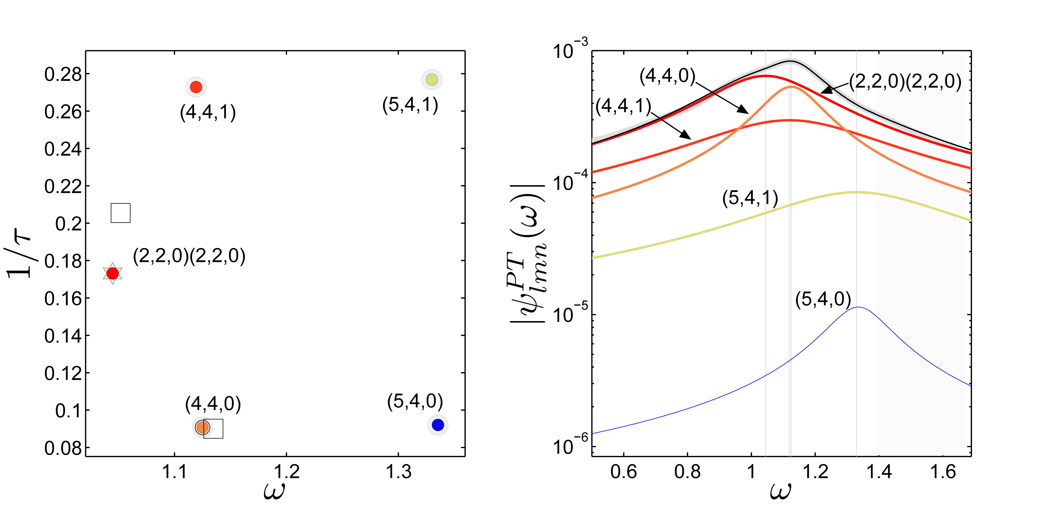 |
Similarly, appears to be dominated by five QNM terms. As expected from single-mode fitting, the fundamental modes generally dominate. However, multimode fitting reveals overtones, and in the case of , an apparent second order QNM. For reference, we have overlayed the results of the modified Prony method in Fig. 6’s lower left panel.
Importantly, like our test case (Table 1), the residual errors for these cases are times smaller than single-mode fitting. We find this to be generally true for initially nonspinning BBH systems of symmetric mass-ratio between 0.2500 and 0.0586. In the following section, we use these cases to peer into the new information captured by multimode fitting. We model the mapping between initial binary mass-ratio and QNM excitation.
IV Mapping QNM Excitation with Symmetric mass-ratio
We apply the greedy-OLS algorithm to the ringdown of quasicircular initially nonspinning BBH systems of symmetric mass-ratio between 0.2500 and 0.0586. The result is a map between and . Just as in the case of inspiral, with its reflective symmetry about the orbital plane, we find that for all systems considered; therefore, we only focus on the multipoles.
By applying the greedy-OLS algorithm to our NR ringdown, we are able to catalog the mass-ratio dependence of overtones and apparent second order QNM. We find that, for the initially nonspinning systems studied here, the mirror modes are not significantly excited.151515We will discuss in Sec. V that imposing these modes detracts from the consistency of our results with perturbation theory While many well-resolved QNMs are recovered, for practicality, we only focus on those needed to represent ringdown up to marginal accuracy. We consider these to be QNMs found within the dominant and spherical multipoles (e.g. ), where Kamaretsos:2011aa ; 0707.0301 ; Healy:2013jza . We go on to present a robust phenomenological model for the mapping between and . We start by touching base with current models for .
The phenomenological models proposed by Kamaretsos:2011aa are shown in Fig. 4. This class of model is derived from the single-mode fitting approach mentioned in Sec.II, and only handles while leaving its complex phase to be matched to the phase of after merger 161616On the other hand, a multimode representation of each (Eq.(16)) requires information about both and its complex phase. While the model functions used in Kamaretsos:2011aa capture the qualitative behavior of the first few fundamental QNMs, the current study’s increased resolution in mass-ratio reveals clear systematic deviations from NR results (Fig. 4, left panel). Most prominently, the local minimum in is not captured by
The more recent work of Kelly:2012nd focuses on the mode, and proposes a qualitatively precise model for ,
| (32) |
where , , , and are real valued constants. Despite the success of this map171717Please see Fig. 10 of Kelly:2012nd ., it is not immediately clear why this functional form works so well, and how its effectiveness may be extended to the other QNMs.
Ultimately, a thorough analytic study of QNM excitation, akin to Zhang:2013ksa , may be needed to derive the mapping between and . While such a pursuit is beyond the current study, a connection between and known physics is appropriate.
To approach this problem, we maintain that QNM excitations are, like their PN counterparts, best described by an expansion in the initial binary’s parameters. Here we expand upon Berti:2007zu by considering a beyond leading order summation in symmetric mass-ratio.
First, we note that the relevant181818nonspinning, non-precessing, quasicircular compact binaries. PN strain multipole moments may be written in the form
| (33) |
where
| (34) | ||||
and is the time dependent part of the waveform’s complex phase Foffa:2013gja ; Kidder:2007rt . In seeking to generalize Eq.(33) to QNM excitations, we may begin by expecting that during ringdown, becomes (we revisit this idea in Sec. IV.1). Furthermore, since and strain are related through two time derivatives, the ringdown analogue of Eq.(33) would pick up a factor of
Lastly, rather than Eq.(33)’s overall scaling by , we find it useful to impose that the excitation of each th overtone be proportional to .
Gathering all of these ideas, we propose that, for QNM excitations, Eq.(33) generalizes to
| (35) | ||||
where
| (36) |
and
| (37) |
While we have chosen to encapsulate the intrinsic contribution (Eq.(37)) within , one might also expect additional extrinsic contributions to from the construction of each simulation (e.g. initial binary separation) Hannam:2010ec . Our approach to these dependencies is outlined in Sec.IV.1.
We also notice that our PN inspired model has the immediate advantage of constraining the QNM amplitudes to be zero in the extreme mass-ratio limit, , while imposing that only even QNMs are excited in the equal-mass case where . As a more phenomenological point, we have chosen to model the overtone dependence as an increasing proportionality in to better fit the NR data.
With these conceptual tools at hand, we may now apply Eq.(35) to NR ringdown by constructing a fit for the complex valued , as a function of .
IV.1 Constructing a fit for on
In order to accurately model ringdown according to Eq.(14), both and the overall phase, must be represented. To do so, let us start by focusing on the aspects of Eq.(35) not given by perturbation theory. First, we rearrange Eq.(35) to define
| (38) | ||||
As we expect to be a polynomial with complex coefficients, it might be well captured by standard least-squares fitting methods; however, we are wary that this approach will be ineffective if is not dominated by the phase of the polynomial sum191919For simplicity, we will not separate the Kerr eigenvalues (e.g. the excitation factors Berti:2006wq ) out from the net QNM excitation, . The result is that the polynomial in question approximates the product of two functions. One, the excitation factor, is independent on the initial parameters. The other is entirely dependent on the initial parameters. .
With this in mind, if we refer to the intrinsic polynomial phase as , and the additional extrinsic contribution as , then
| (39) |
Physically, if there is a preferred azimuthal direction postmerger, then one might expect it to dominate .
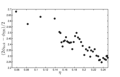
In practice, we find this preferred direction is set by the kick velocity. For the simulations considered here, the kick velocity is always within the orbital plane of the initial binary, giving . The direction of the kick velocity with respect to the simulation frame is then . In this sense, we find that the extrinsic part of ’s complex phase is given by
| (40) |
Together with Eq.(39) and Eq.(36), we now have that
| (41) |
Note that changes in the line of sight about the BH’s final spin direction affect and in the same way. Put differently, redefining Eq.(13)’s to be effectively adds to both sides of Eq.(41). This leaves Eq.(41)’s as an orientation independent quantity (e.g. independent of the observer’s location in the initial binaries orbital plane).
However, is not purely intrinsic. As we have written it in Eq.(41), not only encapsulates the difference between the final kick orientation and QNM phase, but also how each QNM’s phase has evolved up to the start of the fitting region , . This is discussed further in Sec. V.1.
Using the QNM, we find that
| (42) |
This gives . The regularity of approximation across different mass-ratios is briefly discussed in Sec. V.3.
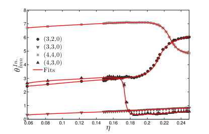
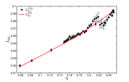
We may therefore construct by evaluating Eq.(43), and applying it to the magnitude of given by Eq.(38). This allows for the simultaneous least-squares fitting of ’s magnitude and phase. Here we have used MATLAB’s . By increasing the order of the polynomial fit until the residual error [Eq.(21)] changes by less than , we find that are well fit by polynomials of order for the considered range of . Figure 7 displays the broad effectiveness of our fitting , and then transforming back to to calculate . Similarly, Fig. 8 displays the corresponding intrinsic phases and their fits.
For each local minimum in Fig. 7, there is a corresponding phase transition in Fig. 8. In an approximate sense, this suggests that each may be more appropriately represented as a polynomial function of , which would force to be a local minimum. However, for simplicity, we have tabulated all fitting coefficients according to Eq.(38).
All fitting coefficients are given in Appendix A.
IV.2 Beyond the fundamentals: overtones & second order modes
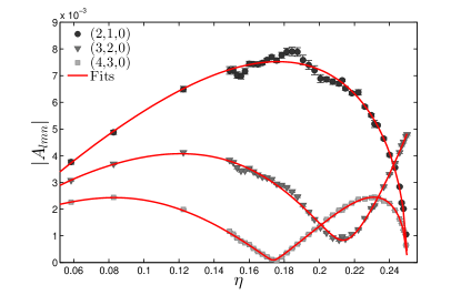
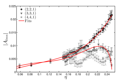
Figure 9 displays estimates for the QNM amplitudes of overtones (top panel) and second order modes (bottom panel) as recovered by the greedy-OLS algorithm. While their existence has been discussed in previous studies (e.g Okuzumi:2008ej ; Nakano:2007cj ; Ioka:2007ak ; Pazos:2010xf ; Zlochower:2003yh ; Pan:2009wj ; Schnittman:2007ij ; Taracchini:2013rva ; Buonanno:2006ui ), we present for the first time their characterization with symmetric mass ratio.
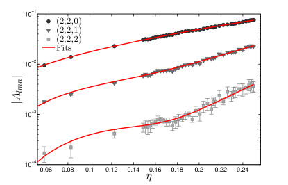
The fitting polynomials for the overtones were found to be of order in . The case is a clear exception, requiring at least an eighth order fit. While we find that many of our estimates of display a localized increase between , displays a significant decrease which makes its dependence possibly inconsistent with Eq.(35). As discussed in Sec.V.1, this is likely due to the definition of ringdown start time in terms of the initial rather than final mass scale.
Given the limitations of our NR runs, we consider these oscillations to be numerical, rather than physical. A similar oscillating trend is observed in the apparent excitation (Fig. 9). We discuss the likely source for these oscillations in the next section (Sec. V.3).
 |
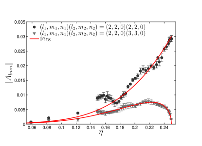 |
While the overtones decay faster (e.g. Fig. 6), their functional form largely mirrors their counterparts (Fig. 7). Similarly, the functional form of the second order modes appears consistent with the notion that each second order mode is largely driven by products of two first order modes Ioka:2007ak . Quantitatively, we expect that each should be proportional to the product of some and
| (44) |
Under this caveat, we model the second order modes according to
| (45) | ||||
where, given and from the first order fits, is the only undetermined parameter.
Upon using a standard root finding algorithm to solve for , we find qualitatively good agreement between our raw estimates for and Eq.(45). While Fig. 9 displays and cases, other less dominant and poorly resolved candidates were detected.
All fitting coefficients are given in Appendix A.
V Consistency with Perturbation Theory and Result Limitations
|
|
 |
 |
While we have developed a method for the estimation of QNM excitation coefficients, this alone does not guarantee the consistency of our results with perturbation theory. This is primarily due to the fact that the QNMs and their related functions are not complete (e.g. gr-qc/9810074 ). In particular, the decaying sinusoids are overcomplete, making it, in principle, possible to achieve an arbitrarily good fit to Eq.(16) with many different combinations of decaying sinusoids. However, the effectiveness of the greedy-OLS method described in Sec. III hinges not on the completeness of the QNMs, but on the uniqueness of the Fourier transform (Eq.(28)), which the algorithm seeks to approximate up to numerical accuracy by focusing only on the sparse QNM frequencies suggested by perturbation theory202020 The greedy-OLS algorithm uses only a handful of frequencies to estimate the Fourier Transform at all frequencies. We find that applying the greedy-OLS algorithm with the QNM frequencies corresponding to a different physical spin does not yield good fits..
Even so, results for may be intrinsically biased if the data are not actually dominated by QNMs. This is the case if the fitting region is chosen either too close to the merger regime, or so far away that irregular numerical noise dominates. For this reason, independent measures of the ’s consistency with perturbation theory are needed. In this section we consider two such measures, and discuss the limitations of our results.
V.1 Fitting region effects
The first estimate of consistency is mentioned at the end of Sec. III.1-14: the effect of ringdown start time, , on . Here we will discuss the effect of on from two perspectives.
Changing Scales.—
On one hand, we may ask why defining relative to the peak luminosity of has been found to yield well-behaved maps between initial binary parameters and QNM excitations. For example, if one defines relative to the peak of rather than its luminosity, then seemingly irregular oscillations are introduced into the dependence of each fundamental mode’s on symmetric mass-ratio. This suggests that there is something about the peak luminosity that serves as a consistent reference for how the system is evolving in the ringdown regime. This postulate is supported by our analysis of each phase in Sec. IV, where we found that when using the peak luminosity as a reference point, the complex phase of each was dependent on time the systems final kick direction with an offset of that is largely independent of initial parameters (Eq.(43)). This means that the phase evolution of each ringdown waveform, relative to the time of the peak luminosity, is approximate for the systems considered here. In other words, the choice to measure time relative to the peak luminosity appears to be approximately the same as choosing such that is constant.
However, there is a discrepancy here: we have chosen in units of the system’s Arnowitt-Deser-Misner (ADM) mass Kamaretsos:2012bs , not the final black hole mass , meaning that while the physical scale of the system() changes, our reference length stays fixed. This along with the dependence of each QNM frequency on the final system state, , should contribute to a systematically varying . The systematic dependence of is shown in Fig. 11 against ( is proportional to ).
As with choosing the peak of rather than its luminosity as a reference point, we might expect seemingly irregular oscillations to appear in the dependence of some . In particular, while further study is needed, the above argument is a likely explanation for the fluctuations of some modes around (e.g. and in Fig. 7, and the modes in Fig. 9).
Different Start Times.—
On the other hand, different fitting regions incur different amounts of numerical noise which may bias results. Therefore we have chosen to quantify this measurement error by considering different fitting regions, and then rescaling our results to be relative to after the peak in ’s luminosity. This measure of consistency answers the question “How much does the recovered QNM behave like a damped sinusoid?” and may be quantified by rescaling according to its complex QNM frequency
| (46) |
In the ideal case, where the estimated behaves exactly as a decaying sinusoid from to , Eq.(46) becomes an equality. This method was utilized to make the error bars throughout this paper.
While we find that the effects of choosing different are inherently systematic212121To the left of ringdown is the nonlinear merger, and to the right is numerical noise., they are also indicative of an optimal start of ringdown that is generally about after the peak luminosity in (Appendix B); however, in some cases the effective ringdown fitting may be performed up to after the peak luminosity. An expanded description of fitting region effects is given in Appendix B.
V.2 Inner-product ratios
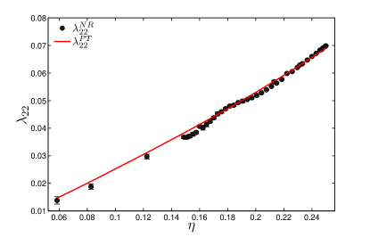
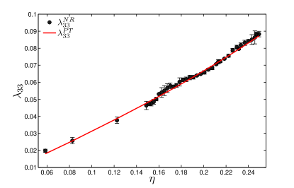
An additional consistency test may be performed by taking advantage of Eq.(16) for different Kelly:2012nd . Noting that any QNM may be found within multiple of the same , it follows that the ratio of their mixing coefficients may be estimated from fitting results, and then compared to analytic calculations via Eq.(17).
For example, in the case of and , Eq.(16) gives that
and
By comparing terms, and recalling that the greedy-OLS algorithm gives a measure for terms in the above sum via Eq.(27)
we see that the ratio, may be estimated directly from the results of multimode fitting. For brevity, we shall limit our discussion to the fundamental modes. For clarity, we will make a distinction between the perturbation theory result derived from Eq.(17)
| (47) |
and the multimode fitting estimate
| (48) | ||||
The three panels of Fig. 10 compare to for . Because is insensitive to waveform phase, we have included results for three waveforms with lower symmetric mass-ratios.
While consistency between perturbation theory and our numerical results is seen in all cases, our estimate does systematically deviate from by roughly on . As suggested by our discussion in Sec. II.3, we consider this deviation to be the result of approaching the magnitude of numerical noise. Moreover, this deviation was found to be exacerbated by the addition of mirror modes(Sec. I.2), the removal of the second order modes, or both.
V.3 Limitations of results
While finite spatial and temporal NR resolution limits the frequencies and multipoles that we are able to consider, we find that our results are stable with respect to the resolutions discussed in Sec. II.3. This also suggests that gauge and near-field effects are not significantly manifested for the majority of our results222222See (Kelly:2012nd, ) for an expanded discussion.. However our consideration of the apparent second order modes carries a more basic limitation: we currently lack detailed knowledge about their structure. Moreover, our lacking many simulations in the very unequal mass-ratio regime presents another limitation.
Second Order Modes.—
As analytic calculations of second order Kerr QNMs are lacking, there exists a tension in the existing literature.
On one hand, analytic studies such as that of Ioka and Nakano Ioka:2007ak suggest that second order perturbations result in QNMs proportional by products of two first order modes. On the other hand, Pazos et al Pazos:2010xf found that, for spherically symmetric initial data, scalar wave scattering off of a Schwarzschild black hole results in second order excitations whose frequencies are the same as those of first order modes.
In this study (Sec. IV.2) we find second order excitations that appear to be largely driven by two first order QNMs, with frequencies that are sums of two first order frequencies. However, as our analysis approach has been designed to only extract spheroidal information post-merger, it cannot directly untangle mode coupling effects that would be consistent with Pazos:2010xf . Therefore, our findings may indeed be consistent with both Pazos:2010xf and Ioka:2007ak . We expect that an analytic study, analogous to Leaver’s work leaver85 , but for second order Kerr perturbations Campanelli:1998jv , may elucidate the matter.
Among the subtleties that should be addressed, we expect the degeneracy of the sum and difference tone spectrum to play an important role: when considering the entire set of possible second order modes, one quickly finds exact or near degeneracies between QNM frequencies with and . Here, the second order modes with the lowest indices, such as (2,2,0)(2,2,0) and (2,2,0)(3,3,0), are not only free from degeneracy at this level, but appear to be the most prominent.
Very unequal mass-ratios.—
Lastly, in regards to our fits for QNM excitation on symmetric mass-ratio, a more basic limitation is the inability to include many points in the very unequal mass-ratio regime (). Therefore, while the fits presented in Sec. IV have been constructed to adhere to the extreme mass-ratio limit, they are, conservatively, only valid within the presented range of .
VI Discussion of Results
In this section, we comment on the potential relevance of subdominant QNMs to ringdown templates and the relevance of our results to perturbation theory.
VI.1 Perturbation theory comments
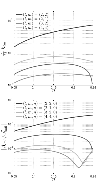
Pending an analytic description of QNM excitation for initially nonspinning, quasicircular BBH merger, akin to Zhang:2013ksa , and a better understanding of the higher order Kerr spectrum, akin to (Zimmerman:2014aha, ), we have found that a PN-like prescription effectively models QNM excitation for the systems studied. The success of this model suggests that a well-defined analytic description exists, and that its predictions may be directly compared to the fitting coefficients in Equations (2-10). When directly compared to its PN counterparts, our model also illuminates the qualitative differences between the inspiral regime, where PN is valid, and the postmerger ringdown regime.
In particular, Fig. 12 shows the qualitative differences between the spherical multipolar GW emission predicted by PN (top panel), and the fundamental spheroidal emission (bottom panel) presented here. On one hand, similarities between the QNMs and their PN counterparts may suggest that they are connected by a largely linear process. On the other hand, the clear differences between PN predictions, and the and QNMs may suggest a region of nonlinear response between and . Further study is needed to precisely clarify whether or not this is the case.
Despite our current limited understanding of the underlying physics, the local minima seen in Fig. 12 suggest that the and QNMs are less likely to be relevant for detection in the 2:1 mass-ratio () regime. This point, in addition to our descriptions of the overtones and second order modes (Sec. IV), allows us to make qualitative comments on the relevance of QNMs to template accuracy and mode detectability.
VI.2 Template comments
While template accuracy and mode detectability are topics whose full treatment is beyond the current work, we are able to briefly comment on the impact of subdominant QNMs on the signal to noise ratio (SNR) of ringdown signals. To do so, we will reconsider the 2:1 mass-ratio binary discussed in the introduction (Fig. 1).
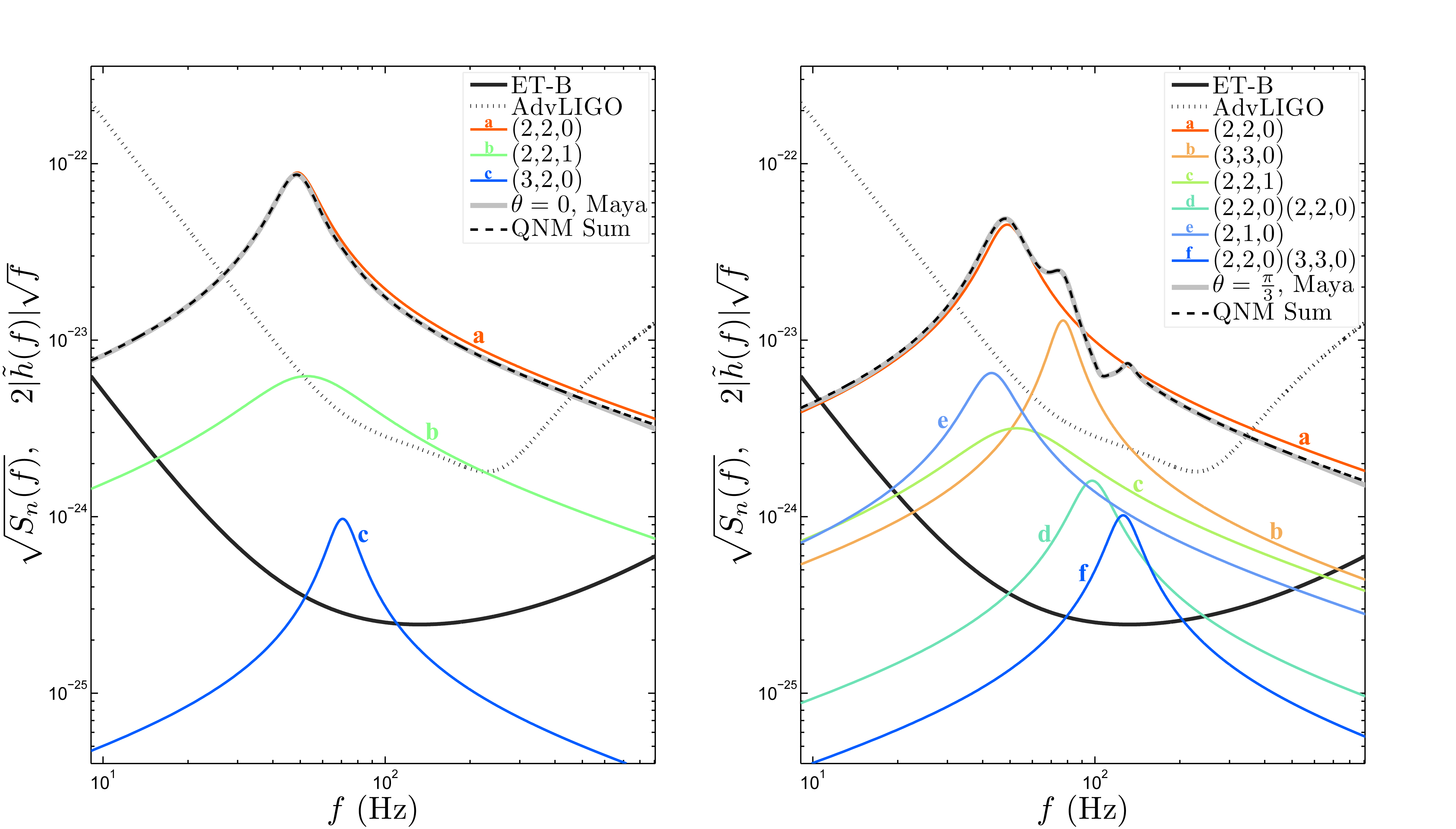
Specifically, let us contemplate an idealized scenario where a ringdown-only template is being used to search for a potential signal as observed by either the Einstein Telescope (ET), or Advanced LIGO (Adv. LIGO). For simplicity we will assume that either detector is equally sensitive over the solid angle, and that there are no glitches in detector sensitivities as presented in Refs. Ajith:2009fz ; Mishra:2010tp . To completely constrain our example, we will consider only templates made with binary parameters identical to that of the signal: final mass 350 , at a distance of 100 Mpc, initially nonspinning, , and quasicircular. We are only interested in the effect of subdominant QNMs on the estimated SNR.
If the signal, , is the frequency domain counterpart of Fig. 1’s waveform, and the template, , is composed of some superposition of QNMs according to the Fourier transform of Eq.(14), then the SNR is given by
| (49) |
where
| (50) |
and is the power spectral density (PSD) of the detected noise Pekowsky:2013ska ; Ajith:2009fz ; Mishra:2010tp .
In the best case scenario, where the signal and template are identical, takes on its maximal value, . Table 2 lists the values of for the orientations shown in Fig. 1.
| Adv. LIGO | ET | |
| 10.58 | 160.79 | |
| 6.20 | 94.29 | |
We now ask which QNMs contribute the most to the total SNR for each of the cases above. To answer this question, we sequentially determine which -mode template recovers the largest percent of . For example, if we denote the recovered SNR of each -mode template to be , then in the case of Adv. LIGO, the 1-mode template that recovers the largest percentage of contains only the QNM. This is the case for , where , and for , where . If we ask which additional QNM results in the largest at , then proves to be the next most important, with . Taking another step forward, we find that the best 3-mode template for Adv. LIGO at includes the , and QNMs, with an SNR of .
| Mode | Adv. LIGO | ET | |||
|---|---|---|---|---|---|
Table 3 lists the percentages of recovered up to the 6-mode template for and up to the 3-mode template for . Figure 13 is a graphical representation of Table 3, and displays each frequency domain QNM against the ET and Adv. LIGO PSDs.
This simple numerical experiment suggests that the greater the angle between the detector’s line of sight and the BH’s final spin direction, the more QNM information is needed to model the signal up to of . While the orientation dependence and impact of multipoles with on detectability is a topic of active interest Healy:2013jza ; Pekowsky:2012sr ; Capano:2013raa , and previous studies of adding fundamental QNMs of to ringdown-only templates have suggested a significant effect on event loss Berti:2007zu ; Caudill:2011kv , our example demonstrates that the overtone may play a meaningful role. Further study, similar to Berti:2007zu , is needed to better quantify its significance.
Intriguingly, although Table 3 shows that the second order QNMs may only add a minuscule amount to the total SNR, their contribution to the frequency domain features in Fig. 13 raises the possibility of their being identified postdetection.
Finally, in light of the QNM amplitude and phase results presented in Sec. III.2, our toy example also allows us to consider what information about the remnant BH may be learned. It is well known that the scaling of QNM frequencies with remnant mass means that the detection of at least two QNM frequencies is required to estimate the final mass and spin of the system Berti:2009kk ; Berti:2007zu ; Berti:2005ys ; Kamaretsos:2012bs ; Gossan:2011ha . This information, along with the relative amplitudes may also yield information about the initial binary, and perhaps even final spin orientation Kamaretsos:2011aa ; Kamaretsos:2012bs . Of the current study, if two QNM frequencies are detected, allowing for the identification of each frequency’s , then a rearrangement of Eq.(42) suggests that information about the recoil angle relative to the line of sight may also be estimated via
| (51) |
The applicability of this potential measure is the subject of a future study.
VII Conclusion
Our in-depth analysis of NR entrance into ringdown has provided us with a wealth of information about the excitation of QNMs. We have found evidence for nonfundamental spheroidal QNM excitations within the residuals of single-mode QNM fits (Sec. II.2). By developing a method to estimate these spheroidal components (Sec. III.1), we have presented a review of QNM excitations including and beyond the fundamentals, and we have discovered that the phase of these excitations is affected by the remnant BH’s final kick direction (Sec. IV.1).
QNM excitations are well modeled by a PN-like expansion (Sec. IV), and that our estimates for the excitation amplitudes are largely consistent with perturbation theory, within the limits of knowledge and numerical accuracy available at the time of this study (Sec. V).
To make our results available for the construction of ringdown related GW templates, we have tabulated related fitting coefficients in Appendix A.
We studied the relevance of our results for GW detection with the ringdown of a 2:1 mass-ratio system of initially nonspinning BHs. For this case, we find that the , overtone is the most dominant, and that that it is the second most significant QNM when the remnant BH is observed along its final spin axis (Fig. 13 left panel). This case also demonstrates that the apparent second mode, while minuscule in comparison to its first counterpart, may be more significant than higher QNMs at similar frequencies (Fig. 13 right panel). Moreover, this case is consistent with the expectation that as the line of sight deviates from the final BH spin direction, more QNMs are needed to accurately represent the signal (Table 3).
But as informative as our example 2:1 mass-ratio system may be, its shortcoming are clear. It demonstrates that when modeling ringdown the can play a role comparable to that of the higher fundamental QNMs (Table 3), but to solidify this statement, and it’s relevance to high mass templates, a full orientation study is needed. We have also seen that apparent second order QNMs might contribute to ringdown’s frequency domain features (Fig. 13), but the full extent to which these modes are relevant cannot be assessed without more accurate NR simulation, and a better understanding of the second order structure of Kerr perturbations. Intriguingly, we have also seen that QNM phase carries information of how the remnant BH is oriented relative to its recoil velocity. While our example system demonstrates that this might allow for an estimation of the recoil direction relative to the line of sight, the scope of the estimation as presented here is only a first step. We look forward to the exploration of this possibility in future work.
VIII Acknowledgments
We are very grateful to Kostas Kokkotas, Pablo Laguna, Vitor Cardoso, Emanuele Berti, Sam Finn and Larne Pekowsky for their helpful input and discussion. We also gratefully acknowledge to support of NSF Grants No. 0955825 and No. 1212433. Numerical simulations were carried out at Teragrid TG-PHY120016 and on the CRA Cygnus clusters.
Appendix A Fitting Coefficients for QNM Excitations
For convenience, here we have collected all fitting formulas and related coefficients. In particular, if one is interested in the QNM excitations from initially nonspinning, quasicircular binary black hole coalescence, then we present the following algorithmic description to apply the model presented in Sec. IV. For additional convenience, a basic usage and plotting example has been made available in reference London:2016err_web.
The primary inputs of our model are the binary’s component masses, and . The primary output of our model is the ringdown portion , starting 10 () after the peak luminosity in the spherical multipole. Therefore, throughout what follows, corresponds to 10 () after the spherical multipole, and values of are to generally be considered outside of the fit’s domain of applicability.
First, given and , one may calculate the symmetric mass-ratio via
With the symmetric mass-ratio, one may use a phenomenological fitting formula to quickly estimate the remnant BH’s final mass, , and dimensionless spin, . While we present fitting formulas in Appendix C, an alternative formula may be found in Rezzolla:2007rd .
Now with the final BH’s parameters at hand, individual QNM frequencies,
may be most readily obtained by using the fitting formulas presented in Berti:2005ys . Alternatively one may use the tabulated values for available at Berti:2005ys_web .
We have that estimates for the complex QNM excitation factors, , may be found by evaluating the following series of equations:
| (52) |
| (53) |
For the second order QNMs discussed in Sec. IV.2, we have that
where for the (2,2,0)(2,2,0) mode we find that
and for the (2,2,0)(3,3,0) mode,
Keeping in mind that all tabulated coefficients correspond to (), the full time domain ringdown waveform may be calculated by first evaluating the spheroidal harmonics, (via leaver85 ), then evaluating
where
Alternatively, one may calculate the spherical multipole moments by evaluating
where
While we have suppressed the second order notation for simplicity, one may again impose the notion that each full second order QNM corresponds to products of two first order modes. With the two expressions for and above, we have completed our algorithmic description for calculating ringdown waveforms using the initial binary’s component masses.
While our discussion thus far has been limited to first and fundamental overtones, and , it should also be noted that consistent evidence for the , , overtone may be readily observed by considering fitting regions closer to the luminosity. Figure 14 displays this overtone scaled relative to (). Though the general trend is reminiscent of the and overtones, the mode’s faster decay rate corresponds to larger variation with fitting region (e.g. larger error bars).
Appendix B The Start of Ringdown
While it is not possible to define an absolute start of ringdown, we may make a practical definition by asking which potential ringdown region is best modeled by QNMs only.
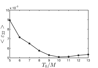
This question may be addressed by finding a local minimum in residual error with respect to fitting region start time. To this end let us consider the multipole which is least effected by numerical errors: . Figure 15 shows its residual error [Eq.(21)] on symmetric mass-ratio. The trend observed here is inherently systematic as, when moving towards the peak in radiation, the data are no longer dominated by QNMs, while, when moving away from the peak, numerical noise eventually dominates.
Consequently, although there is a visible minimum at , it is not the global minimum, as fluctuates in the numerical noise following . However, nevertheless gives us a practical starting point within which the majority of is above the numerical noise floor.
Appendix C Final Mass and Spin
As noted in Rezzolla:2007rd , the final mass and spin dependence on initial binary symmetric mass-ratio may be well fit by a polynomial in . Alternatively, the more recent study, Ref. Healy:2014yta , shows that the final BH parameters may also be well modeled as a power series in . Here, we present a methodologically different fit than that presented in Rezzolla:2007rd and Healy:2014yta , while maintaining the parametrization of Rezzolla:2007rd . Specifically, when fitting final dimensionless spin, , we choose to directly impose the boundary condition that as , . In particular, we fit
| (54) |
Similarly, when fitting final mass, , we choose to directly impose the boundary condition that as , . In particular, we fit
| (55) |
The fitting result for is shown in Fig. 2. Fitting coefficients are tabulated in Table 4. While the fitting results here are consistent with Rezzolla:2007rd and Healy:2014yta within their fit’s domain of applicability (deviations are within 1% of the values reported), we expect that the forms given in 54 and 55 bias the fit towards the physically correct solution outside of the fitting domain.
Consistency with multimode Fit.—
The numerical values used to make the above fits (Table 4) were calculated using the isolated horizon formalism Frauendiener:2011zz . However, final BH mass and spin may also be estimated using ringdown fitting (e.g. Hannam:2010ec ; Berti:2007zu ). For the numerical runs considered here, we find that single mode fitting recovers the horizon estimate to within , while multimode fitting recovers the horizon estimate to within . This level of agreement is within the numerical error of the isolated horizon estimate.
References
- (1) J. Abadie et al., “Predictions for the Rates of Compact Binary Coalescences Observable by Ground-based Gravitational-wave Detectors,” Class.Quant.Grav., vol. 27, p. 173001, 2010.
- (2) K. Belczynski, M. Dominik, T. Bulik, R. O’Shaughnessy, C. Fryer, et al., “The effect of metallicity on the detection prospects for gravitational waves,” 2010.
- (3) C. K. Mishra, K. Arun, B. R. Iyer, and B. Sathyaprakash, “Parametrized tests of post-Newtonian theory using Advanced LIGO and Einstein Telescope,” Phys.Rev., vol. D82, p. 064010, 2010.
- (4) P. Ajith and S. Bose, “Estimating the parameters of non-spinning binary black holes using ground-based gravitational-wave detectors: Statistical errors,” Phys.Rev., vol. D79, p. 084032, 2009.
- (5) M. Ruiz, M. Alcubierre, D. Núñez, and R. Takahashi, “Multiple expansions for energy and momenta carried by gravitational waves,” General Relativity and Gravitation, vol. 40, pp. 1705–1729, 2008.
- (6) The LIGO Scientific Collaboration, the Virgo Collaboration, J. Aasi, B. P. Abbott, R. Abbott, T. Abbott, M. R. Abernathy, F. Acernese, K. Ackley, C. Adams, and et al., “Narrow-band search of continuous gravitational-wave signals from Crab and Vela pulsars in Virgo VSR4 data,” ArXiv e-prints, Oct. 2014.
- (7) W. H. Press and S. A. Teukolsky, “Perturbations of a rotating black hole. ii. dynamical stability of the kerr metric,” Astrophysical Journal, vol. 185, pp. 649–674, 1973.
- (8) E. Leaver, “An Analytic representation for the quasi normal modes of Kerr black holes,” Proc.Roy.Soc.Lond., vol. A402, pp. 285–298, 1985.
- (9) E. Berti, V. Cardoso, J. A. Gonzalez, U. Sperhake, M. Hannam, S. Husa, and B. Brügmann, “Inspiral, merger, and ringdown of unequal mass black hole binaries: A multipolar analysis,” Phys. Rev. D, vol. 76, p. 064034, Sep 2007.
- (10) I. Kamaretsos, M. Hannam, S. Husa, and B. Sathyaprakash, “Black-hole hair loss: learning about binary progenitors from ringdown signals,” Phys.Rev., vol. D85, p. 024018, 2012.
- (11) Maya makes use of the openly available Einstein Toolkit et-web , which is based on the CACTUS cactus-web code structure and CARPET Schnetter-etal-03b mesh refinement. Related subroutines have been generated by the Kranc Husa:2004ip library.
-
(12)
Einstein Toolkit home page:
http://www.einsteintoolkit.org. - (13) Cactus Computational Toolkit home page:http://www.cactuscode.org.
- (14) E. Schnetter, S. H. Hawley, and I. Hawke, “Evolutions in 3D numerical relativity using fixed mesh refinement,” Class. Quant. Grav., vol. 21, pp. 1465–1488, 21 March 2004.
- (15) S. Husa, I. Hinder, and C. Lechner, “Kranc: a mathematica application to generate numerical codes for tensorial evolution equations,” Computer Physics Communications, vol. 174, pp. 983–1004, June 2006.
- (16) A. Taracchini, A. Buonanno, Y. Pan, T. Hinderer, M. Boyle, et al., “Effective-one-body model for black-hole binaries with generic mass ratios and spins,” 2013.
- (17) T. Damour and A. Nagar, “An Improved analytical description of inspiralling and coalescing black-hole binaries,” Phys.Rev., vol. D79, p. 081503, 2009.
- (18) Y. Pan, A. Buonanno, L. T. Buchman, T. Chu, L. E. Kidder, et al., “Effective-one-body waveforms calibrated to numerical relativity simulations: coalescence of non-precessing, spinning, equal-mass black holes,” Phys.Rev., vol. D81, p. 084041, 2010.
- (19) B. J. Kelly and J. G. Baker, “Decoding mode mixing in black-hole merger ringdown,” Phys.Rev., vol. D87, p. 084004, 2013.
- (20) E. N. Dorband, E. Berti, P. Diener, E. Schnetter, and M. Tiglio, “A Numerical study of the quasinormal mode excitation of Kerr black holes,” Phys.Rev., vol. D74, p. 084028, 2006.
- (21) S. Okuzumi, K. Ioka, and M.-a. Sakagami, “Possible Discovery of Nonlinear Tail and Quasinormal Modes in Black Hole Ringdown,” Phys.Rev., vol. D77, p. 124018, 2008.
- (22) J. D. Schnittman, A. Buonanno, J. R. van Meter, J. G. Baker, W. D. Boggs, et al., “Anatomy of the binary black hole recoil: A multipolar analysis,” Phys.Rev., vol. D77, p. 044031, 2008.
- (23) A. Buonanno, G. B. Cook, and F. Pretorius, “Inspiral, merger and ring-down of equal-mass black-hole binaries,” Phys.Rev., vol. D75, p. 124018, 2007.
- (24) J. Healy, C. O. Lousto, and Y. Zlochower, “Remnant mass, spin, and recoil from spin aligned black-hole binaries,” 2014.
- (25) E. Berti, V. Cardoso, and C. M. Will, “On gravitational-wave spectroscopy of massive black holes with the space interferometer LISA,” Phys.Rev., vol. D73, p. 064030, 2006.
- (26) C. V. Vishveshwara, “Stability of the schwarzschild metric,” Phys. Rev. D, vol. 1, pp. 2870–2879, May 1970.
- (27) E. Berti, V. Cardoso, and A. O. Starinets, “Quasinormal modes of black holes and black branes,” Class.Quant.Grav., vol. 26, p. 163001, 2009.
- (28) S. Caudill, S. E. Field, C. R. Galley, F. Herrmann, and M. Tiglio, “Reduced Basis representations of multi-mode black hole ringdown gravitational waves,” Class.Quant.Grav., vol. 29, p. 095016, 2012.
- (29) S. A. Teukolsky, “Perturbations of a rotating black hole. i. fundamental equations for gravitational, electromagnetic, and neutrino-field perturbations,” Astrophysical Journal, vol. 185, pp. 635–648, 1973.
- (30) K. D. Kokkotas and B. G. Schmidt, “Quasi-normal modes of stars and black holes,” Living Review in Relativity, vol. 2, 1999.
- (31) E. Berti, J. Cardoso, V. Cardoso, and M. Cavaglia, “Matched-filtering and parameter estimation of ringdown waveforms,” Phys.Rev.D, vol. 76, p. 104044, 2007.
- (32) M. Campanelli and C. O. Lousto, “Second order gauge invariant gravitational perturbations of a Kerr black hole,” Phys.Rev., vol. D59, p. 124022, 1999.
- (33) H. Nakano and K. Ioka, “Second Order Quasi-Normal Mode of the Schwarzschild Black Hole,” Phys.Rev., vol. D76, p. 084007, 2007.
- (34) K. Ioka and H. Nakano, “Second and higher-order quasi-normal modes in binary black hole mergers,” Phys.Rev., vol. D76, p. 061503, 2007.
- (35) E. Pazos, D. Brizuela, J. M. Martin-Garcia, and M. Tiglio, “Mode coupling of Schwarzschild perturbations: Ringdown frequencies,” Phys.Rev., vol. D82, p. 104028, 2010.
- (36) Y. Zlochower, R. Gomez, S. Husa, L. Lehner, and J. Winicour, “Mode coupling in the nonlinear response of black holes,” Phys.Rev., vol. D68, p. 084014, 2003.
- (37) I. Kamaretsos, “From black holes to their progenitors: A full population study in measuring black hole binary parameters from ringdown signals,” J.Phys.Conf.Ser., vol. 363, p. 012047, 2012.
- (38) I. Kamaretsos, M. Hannam, and B. Sathyaprakash, “Is black-hole ringdown a memory of its progenitor?,” Phys.Rev.Lett., vol. 109, p. 141102, 2012.
- (39) E. W. Leaver, “Spectral decomposition of the perturbation response of the Schwarzschild geometry,” Phys.Rev., vol. D34, pp. 384–408, 1986.
- (40) E. Berti, V. Cardoso, and M. Casals, “Eigenvalues and eigenfunctions of spin-weighted spheroidal harmonics in four and higher dimensions,” Phys. Rev. D, vol. 73, p. 024013, Jan 2006.
- (41) Z. Zhang, E. Berti, and V. Cardoso, “Quasinormal ringing of Kerr black holes. II. Excitation by particles falling radially with arbitrary energy,” 2013.
- (42) R. H. Price, “Nonspherical Perturbations of Relativistic Gravitational Collapse. II. Integer-Spin, Zero-Rest-Mass Fields,” Phys.Rev., vol. D5, pp. 2439–2454, 1972.
- (43) W. Krivan, P. Laguna, and P. Papadopoulos, “Dynamics of scalar fields in the background of rotating black holes,” Phys. Rev. D, vol. 54, pp. 4728–4734, Oct 1996.
- (44) S. A. Teukolsky, “Rotating black holes: Separable wave equations for gravitational and electromagnetic perturbations,” Phys. Rev. Lett., vol. 29, pp. 1114–1118, Oct 1972.
- (45) E. Mitsou, “Gravitational radiation from radial infall of a particle into a Schwarzschild black hole. A numerical study of the spectra, quasi-normal modes and power-law tails,” Phys.Rev., vol. D83, p. 044039, 2011.
- (46) M. A. Scheel, A. L. Erickcek, L. M. Burko, L. E. Kidder, H. P. Pfeiffer, et al., “3-D simulations of linearized scalar fields in Kerr space-time,” Phys.Rev., vol. D69, p. 104006, 2004.
- (47) E. Harms, S. Bernuzzi, and B. Brügmann, “Numerical solution of the 2+1 Teukolsky equation on a hyperboloidal and horizon penetrating foliation of Kerr and application to late-time decays,” Class.Quant.Grav., vol. 30, p. 115013, 2013.
- (48) J. Stewart, “Stability of Kerr’s spacetime,” Proc.Roy.Soc.Lond., vol. A344, pp. 65–79, 1975.
- (49) J. Frauendiener, “Miguel Alcubierre: Introduction to 3 + 1 numerical relativity,” Gen.Rel.Grav., vol. 43, pp. 2931–2933, 2011.
- (50) E. Berti, V. Cardoso, J. A. Gonzalez, and U. Sperhake, “Mining information from binary black hole mergers: a comparison of estimation methods for complex exponentials in noise,” Phys.Rev.D, vol. 75, p. 124017, 2007.
- (51) E. N. Dorband, E. Berti, P. Diener, E. Schnetter, and M. Tiglio, “A numerical study of the quasinormal mode excitation of kerr black holes,” Phys.Rev.D, vol. 74, no. LSU-REL-081806, p. 084028, 2006.
- (52) M. Hannam, S. Husa, F. Ohme, D. Muller, and B. Bruegmann, “Simulations of black-hole binaries with unequal masses or nonprecessing spins: Accuracy, physical properties, and comparison with post-Newtonian results,” Phys.Rev., vol. D82, p. 124008, 2010.
- (53) J. D. Schnittman, A. Buonanno, J. R. van Meter, J. G. Baker, W. D. Boggs, J. Centrella, B. J. Kelly, and S. T. McWilliams, “Anatomy of the binary black hole recoil: A multipolar analysis,” Phys.Rev.D, vol. 77, p. 044031, 2008.
- (54) J. Meidam, M. Agathos, C. Van Den Broeck, J. Veitch, and B. Sathyaprakash, “TIGER’s tail: Testing the no-hair theorem with black hole ringdowns,” 2014.
- (55) P. Ajith, M. Boyle, D. A. Brown, B. Brügmann, L. T. Buchman, et al., “The NINJA-2 catalog of hybrid post-Newtonian/numerical-relativity waveforms for non-precessing black-hole binaries,” Class.Quant.Grav., vol. 29, p. 124001, 2012.
- (56) M. R. Osborne and G. K. Smyth, “A modified prony algorithm for exponential function fitting,” SIAM Journal of Scientific Computing, vol. 16, pp. 119–138, 1995.
- (57) T. H. Cormen, C. E. Leiserson, R. L. Rivest, and C. Stein, Introduction to Algorithms. The MIT Press, 2 ed., 2001.
- (58) O. P. F. Piedra and J. de Oliveira, “Fermion perturbations in string theory black holes,” Classical and Quantum Gravity, vol. 28, no. 8, p. 085023, 2011.
- (59) G. Smyth, “http://www.statsci.org/matlab/mprony.html,”
- (60) D. W. Marquardt, “An algorithm for least-squares estimation of nonlinear parameters,” SIAM Journal on Applied Mathematics, vol. 11, no. 2, pp. 431–441, 1963.
- (61) J. Healy, P. Laguna, L. Pekowsky, and D. Shoemaker, “Template Mode Hierarchies for Binary Black Hole Mergers,” Phys.Rev., vol. D88, p. 024034, 2013.
- (62) S. Foffa, “Gravitating binaries at 5PN in the post-Minkowskian approximation,” 2013.
- (63) L. E. Kidder, “Using full information when computing modes of post-Newtonian waveforms from inspiralling compact binaries in circular orbit,” Phys.Rev., vol. D77, p. 044016, 2008.
- (64) E. Berti and V. Cardoso, “Quasinormal ringing of Kerr black holes. I. The Excitation factors,” Phys.Rev., vol. D74, p. 104020, 2006.
- (65) H.-P. Nollert and R. H. Price, “Quantifying excitations of quasinormal mode systems,” J.Math.Phys., vol. 40, pp. 980–1010, 1999.
- (66) L. Blanchet, G. Faye, B. R. Iyer, and S. Sinha, “The Third post-Newtonian gravitational wave polarisations and associated spherical harmonic modes for inspiralling compact binaries in quasi-circular orbits,” Class.Quant.Grav., vol. 25, p. 165003, 2008.
- (67) A. Zimmerman, H. Yang, Z. Mark, Y. Chen, and L. Lehner, “Quasinormal Modes Beyond Kerr,” 2014.
- (68) L. Pekowsky, R. O’Shaughnessy, J. Healy, and D. Shoemaker, “Comparing gravitational waves from nonprecessing and precessing black hole binaries in the corotating frame,” Phys.Rev., vol. D88, p. 024040, 2013.
- (69) L. Pekowsky, J. Healy, D. Shoemaker, and P. Laguna, “Impact of Higher-order Modes on the Detection of Binary Black Hole Coalescences,” Phys.Rev., vol. D87, p. 084008, 2013.
- (70) C. Capano, Y. Pan, and A. Buonanno, “Impact of Higher Harmonics in Searching for Gravitational Waves from Non-Spinning Binary Black Holes,” 2013.
- (71) S. Gossan, J. Veitch, and B. Sathyaprakash, “Bayesian model selection for testing the no-hair theorem with black hole ringdowns,” Phys.Rev., vol. D85, p. 124056, 2012.
- (72) L. Rezzolla, P. Diener, E. N. Dorband, D. Pollney, C. Reisswig, et al., “The Final spin from the coalescence of aligned-spin black-hole binaries,” Astrophys.J., vol. 674, pp. L29–L32, 2008.
- (73) E. Berti, “http://www.phy.olemiss.edu/ berti/qnms.html,”
