Role of diproton correlation in two-proton emission decay
of the ⁶Be nucleus

Abstract

We discuss a role of diproton correlation in two-proton emission from the ground state of a proton-rich nucleus, ⁶Be. Assuming the three-body structure of $\alpha+p+p$ configuration, we develop a time-dependent approach, in which the two-proton emission is described as a time-evolution of a three-body metastable state. With this method, the dynamics of the two-proton emission can be intuitively discussed by monitoring the time-dependence of the two-particle density distribution. With a model Hamiltonian which well reproduces the experimental two-proton decay width, we show that a strongly correlated diproton emission is a dominant process in the early stage of the two-proton emission. When the diproton correlation is absent, the sequential two-proton emission competes with the diproton emission, and the decay width is underestimated. These results suggest that the two-proton emission decays provide a good opportunity to probe the diproton correlation in proton-rich nuclei beyond the proton drip-line.

I Introduction

The pairing correlation plays an essential role in many phenomena of atomic nuclei 03Brink ; RS80 ; BCS50 ; 96Doba ; 03Dean . In recent years, the dineutron and diproton correlations have particularly attracted a lot of interests in connection to the physics of unstable nuclei 73Mig ; 84Catara ; 91Bert ; Zhukov93 ; OZV99 ; 05Mats ; 06Mats ; 05Hagi ; 10Ois ; 10Pillet . These are correlations induced by the pairing interaction, with which two nucleons are spatially localized. Since the pairing gap in infinite nuclear matter takes a maximum at the density lower than the normal density 06Mats ; 03Dean ; 06Cao ; 07Marg , the dinucleon correlation is enhanced on the surface of nuclei. This property may also be related to the BCS-BEC crossover 06Mats ; 07Marg ; HSCS07 .

Although the dinucleon correlation has been theoretically predicted for some time, it is still an open issue to probe it experimentally. For this purpose, a pair-transfer reaction 91Iga ; 01Oert ; 11Shim and the electro-magnetic excitations 04Fuku ; 06Naka ; 01Myo ; 07Hagi ; 07Bertulani_76 ; 11Ois ; 10Kiku may be considered. However, even though there have been a few experimental indications 06Naka , so far no direct experimental evidence for the dinucleon correlation has been found, mainly due to a difficulty to access the intrinsic structures in bound nuclei without disturbing with an external field.

This difficulty may be overcome by using two-proton (2p-) emission decays (these are referred to as two-proton radio-activities when the decay width is sufficiently small) of nuclei outside the proton drip-line 08Bla ; 12Pfu ; 09Gri_40 . An attractive feature of the 2p-emission is that two protons are emitted spontaneously from the ground state of unbound nuclei, and thus they are expected to carry information on the pairing correlations inside nuclei, including the diproton correlation 05Flam ; 07Bertulani_34 ; 08Bertulani ; 12Maru .

The 2p-radioactivity was predicted for the first time by Goldansky 60Gold ; 61Gold . He introduced the concept of the “true 2p-decay”, which takes place in the situation where the emission of single proton is energetically forbidden. The pairing interaction plays an important role to generate such a situation, lowering the energy of even-Z nuclei. In the true 2p-decay process, the two protons may be emitted simultaneously as a diproton, that is, the diproton decay 60Gold ; 61Gold ; 13Deli . This process should thus intimately be related to the diproton correlation.

Since the time of Goldansky, there has been an enormous progress in the problem of 2p-decays, both experimentally and theoretically, and our understanding of the 2p-decays has been considerably improved08Bla ; 12Pfu ; 09Gri_40 . It has been considered now that the actual 2p-decays are often much more complicated than the simple diproton decays which Goldansky originally proposed 89Boch ; 05Rotu ; 07Mie ; 09Gri_677 ; 09Gri_80 ; 08Muk ; 10Muk ; 12Ego ; 12Gri . Moreover, it has not been completely clarified whether the diproton correlation can be actually probed by observing 2p-decays.

The aim of this paper is to investigate the role of the diproton correlation in 2p-emissions, and discuss a possibility of probing the diproton correlation through the 2p-decays. For this purpose, one needs to handle a many-body meta-stable state, for which the theoretical frameworks can be categorized into two approaches: the time-independent framework 89Bohm ; 28Gamov ; 29Gurney and the time-dependent framework 89Bohm ; 47Kry ; 89Kuku . In the time-independent approach, the decay state is regarded as a pure outgoing state with a complex energy, that is, the Gamow state. The real and the imaginary parts of the complex energy are related to the decay energy and width, respectively. An advantage of this method is that the decay width can be accurately calculated even when the width is extremely small 09Gri_40 ; 01Gri_I ; 97Aberg ; 00Davis . In the time-dependent framework, on the other hand, the quantum decay of a metastable state is treated as a time-evolution of a wave packet 94Serot ; 98Talou ; 99Talou_60 ; 00Talou ; 11Garc ; 11Campo ; 12Pons . An advantage of this method is that the decay dynamics can be intuitively understood by monitoring the time-evolution of the wave packet. These two approaches are thus complementary to each other.

In this paper, we employ the time-dependent approach. This approach has been used in Refs. 94Serot ; 98Talou ; 99Talou_60 ; 00Talou to study one-proton emission decays of proton-rich nuclei. In our previous work 12Maru , we extended this approach to 2p-emission in one-dimension. We here apply this method to a realistic system, that is, the ground state of the ⁶Be nucleus, by assuming the three-body structure of $\alpha+p+p$. The ⁶Be nucleus is the lightest 2p-emitter, where the 2p-emission decay from its ground state has been experimentally studied in Refs. 89Boch ; 09Gri_80 ; 09Gri_677 ; 12Ego . The experimental Q-value of the 2p-emission is $1.37$ MeV 88Ajz ; 02Till , while the ⁵Li nucleus is unbound by 1.96(5) MeV from the threshold of $\alpha+p$ 88Ajz , as shown in Fig. 1. Although the ⁵Li nucleus has a large resonance width of about 1.5 MeV 88Ajz ; 02Till , the ⁶Be nucleus is considered to be a true 2p-emitter. Therefore, the sequential decay via the $\alpha+p$ subsystem plays a minor role, and the effect of the diproton correlation, due to the pairing correlation, may significantly be revealed.

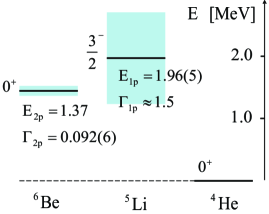
Figure 1: (Color online) The experimental energy scheme of ⁶Be and ⁵Li nuclei with respect to the ground state of ⁴He 88Ajz . The energies and widths are shown in units of MeV.

The paper is organized as follows. In Sec. II, we present the theoretical model and the time-dependent approach within a quantum three-body model. The calculated results for ⁶Be are shown in Sec. III. We also discuss the role of pairing correlation in the 2p-emission. We then summarize the paper in Sec. IV.

II Formalism

II.1 Three-body model Hamiltonian

In order to describe the 2p-emission from the ground state of ⁶Be, we consider a three-body model which consists of an $\alpha$-particle as the spherical core nucleus and two valence protons. As in Refs. 91Bert ; 05Hagi ; 10Ois ; 11Ois , we employ the so called V-coordinate indicated in Fig. 2. Subtracting the center of mass motion of the whole nucleus, the total Hamiltonian reads

$$H_{\rm 3b} = h_{1}+h_{2}+\frac{\bm{p}_{1}\cdot\bm{p}_{2}}{A_{\rm c}m}+v_{\rm pp}(\bm{r}_{1},\bm{r}_{2}),$$ (1)

$$h_{i} = \frac{\bm{p}_{i}^{2}}{2\mu}+V_{\rm cp}(r_{i})\;\;\;\;(i=1,2),$$ (2)

where $h_{i}$ is the single particle (s.p.) Hamiltonian between the core and the $i$-th proton. $\mu\equiv mA_{\rm c}/(A_{\rm c}+1)$ is the reduced mass where $m$ and $A_{\rm c}$ are the nucleon mass and the mass number of the core nucleus, respectively. The interaction between $\alpha$ and a valence proton, $V_{\rm cp}$, consists of the nuclear potential $V_{\rm WS}$ and the Coulomb potential $V_{\rm Coul}$,

$$V_{\rm cp}(r_{i})=V_{\rm WS}(r_{i})+V_{\rm Coul}(r_{i}).$$ (3)

For the Coulomb part of the potential, $V_{\rm Coul}$, we use the one appropriate to a uniformly charged spherical alpha particle of radius $r_{c}=1.68$ fm. For the nuclear part, $V_{\rm WS}$, on the other hand, we use the Woods-Saxon parametrization given by

$$V_{\rm WS}(r)=V_{0}f(r)+U_{ls}(\bm{l}\cdot\bm{s})\frac{1}{r}\frac{df(r)}{dr},$$ (4)

where

$$f(r)=\frac{1}{1+e^{(r-R_{0})/a_{0}}}$$ (5)

with $R_{0}=r_{c}$ and $a_{0}$ = 0.615 fm. We use the depth parameters of $V_{0}=-58.7$ MeV and $U_{ls}=46.3$ ${\rm MeV\cdot fm^{2}}$. This potential yields the resonance energy and the width of the $(p_{3/2})$-channel for $\alpha-p$ scattering of $E_{r}(p_{3/2})=1.96$ MeV and $\Gamma_{r}(p_{3/2})=1.56$ MeV, respectively. These values are compared with the experimental data, $E_{r}(p_{3/2})=1.96(5)$ MeV and $\Gamma_{r}(p_{3/2})\sim 1.5$ MeV (see Fig.1) 88Ajz . We note that this resonance state is quite broad and there has been some ambiguity in the observed decay width 88Ajz ; 02Till ; 00Hoef ; 09Shir .

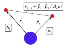
Figure 2: (Color online) The V-coordinate for three-body system.

For the proton-proton interaction, $v_{\rm pp}$, we use the Minnesota potential 77Thom together with the Coulomb term for point charges:

$$v_{\rm pp}(\bm{r}_{1},\bm{r}_{2})=v_{0}e^{-b_{0}r_{12}^{2}}+v_{1}e^{-b_{1}r_{12}^{2}}+\frac{e^{2}}{r_{12}},$$ (6)

where $r_{12}=\left|\bm{r}_{1}-\bm{r}_{2}\right|$. For $b_{0},b_{1}$ and $v_{1}$, we use the same parameters introduced in the original paper 77Thom , as summarized in Table 1. On the other hand, the strength of the repulsive term, $v_{0}$, is adjusted so as to reproduce the empirical Q-value for the two-proton emission, as we will discuss in Sec. III.

	$b_{0}$ (fm-2)	$b_{1}$ (fm-2)	$v_{1}$ (MeV)
$S=0$	1.48	0.639	$-178.0$
$S=1$	1.48	0.465	$-91.85$

Table 1: The values of $b_{0},b_{1}$ and $v_{1}$ in the Minnesota potential given by Eq.(6). $S$ indicates the combined spin of the two protons.

II.2 Uncorrelated Two-proton Basis

Each s.p. state satisfying $h_{i}\phi_{a}(\bm{r}_{i})=\epsilon_{a}\phi_{a}(\bm{r}_{i})$ is labeled by $a=\left\{n_{a},l_{a},j_{a},m_{a}\right\}$, that is, a combination of the radial quantum number $n$, the orbital angular momentum $l$, the spin-coupled angular momentum $j$ and its z-component $m$. Using these s.p. wave functions, one can construct the uncorrelated basis for the two protons coupled to an arbitrary spin-parity, $J^{\pi}$, where the coupled angular momentum $J$ is given by $J=j_{a}\oplus j_{b}$ and the total parity $\pi$ is given by $\pi=(-)^{l_{a}+l_{b}}$. That is,

$$\Phi_{ab}^{(J^{\pi})}(\bm{r}_{1},\bm{r}_{2})=\hat{\mathcal{A}}\left[\phi_{a}(\bm{r}_{1})\otimes\phi_{b}(\bm{r}_{2})\right]^{(J^{\pi})},$$ (7)

where $\hat{\mathcal{A}}$ is the anti-symmetrization operator. In this work, we assume that the core nucleus always stays in the ground state with the spin-parity of $0^{+}$. Thus the uncorrelated basis given by Eq.(7) are reduced only to the $J^{\pi}=0^{+}$ subspace, since the ground state of ⁶Be also has the spin-parity of $0^{+}$. That is,

$$\Phi_{ab}^{(0^{+})}(\bm{r}_{1},\bm{r}_{2})=\Phi_{n_{a}n_{b}lj}(\bm{r}_{1},\bm{r}_{2})$$ (8)

$$\phantom{00}=\frac{1}{\sqrt{2(1+\delta_{n_{a},n_{b}})}}\sum_{m}C(j,m;j,-m\mid 0,0)$$

$$\phantom{0000}\left[\phi_{n_{a}ljm}(\bm{r}_{1})\phi_{n_{b}lj-m}(\bm{r}_{2})\right.$$

$$\phantom{0000}\left.+\phi_{n_{a}ljm}(\bm{r}_{2})\phi_{n_{b}lj-m}(\bm{r}_{1})\right].$$ (9)

Notice $l_{a}=l_{b}$, $j_{a}=j_{b}$ for the $0^{+}$ state. In the following, for simplicity, we omit the superscript $(0^{+})$ and use a simplified notation, $\ket{\Phi_{M}}$, for the uncorrelated basis given by Eq. (9), where $M=(n_{a},n_{b},l,j)$.

The eigen-states of the three-body Hamiltonian, $H_{\rm 3b}$, can be obtained by expanding the wave function on the uncorrelated basis,

$$\ket{E_{N}}=\sum_{M}U_{NM}\ket{\Phi_{M}},$$ (10)

where the expansion coefficients, $U_{NM}$, are determined by diagonalizing the Hamiltonian matrix for $H_{\rm 3b}$. The state $\ket{E_{N}}$ then satisfies $H_{\rm 3b}\ket{E_{N}}=E_{N}\ket{E_{N}}$ in a truncated space.

All our calculations are performed in the truncated space defined by the energy-cutoff, $\epsilon_{a}+\epsilon_{b}\leq E_{\rm cut}=40$ MeV. The continuum s.p. states are discretized within the radial box of $R_{\rm box}=80$ fm (notice that the states $\ket{E_{N}}$ are also discretized). For the angular momentum channels, we include from $(s_{1/2})^{2}$ to $(h_{11/2})^{2}$ configurations. In order to take into account the effect of the Pauli principle, we exclude the bound 1$s_{1/2}$ state from Eq.(10), that is given by the protons in the core nucleus. We have confirmed that our conclusions do not change even if we employ a larger value of $E_{\rm cut}$ and/or include higher partial waves.

II.3 Time-Dependent Method for Two-Proton Decay

Assuming the 2p-emission as a time-dependent process, we carry out time-dependent calculations for the three-body system, ⁶Be. For this purpose, we first need to determine the initial state, $\ket{\Psi(t=0)}$, for which the two valence protons are confined inside the potential barrier generated by the core nucleus. That is, the 2p-density distribution at $t=0$ has almost no amplitude outside the potential barrier. In order to construct such initial state, we employ the confining potential method, which will be detailed in the next section.

The initial state so obtained can be expanded with the eigen-states of $H_{\rm 3b}$, that is, $\ket{E_{N}}$ given by Eq. (10) as

$$\ket{\Psi(0)}=\sum_{N}F_{N}(0)\ket{E_{N}}.$$ (11)

After the time-evolution with the three-body Hamiltonian $H_{\rm 3b}$, this state is evolved to

$$\ket{\Psi(t)}=\exp\left[-it\frac{H_{\rm 3b}}{\hbar}\right]\ket{\Psi(0)}=\sum_{N}F_{N}(t)\ket{E_{N}},$$ (12)

where

$$F_{N}(t)=e^{-itE_{N}/\hbar}F_{N}(0).$$ (13)

Notice that the state $\ket{\Psi(t)}$ can also be expanded on the uncorrelated basis as,

$$\ket{\Psi(t)}=\sum_{M}C_{M}(t)\ket{\Phi_{M}},$$ (14)

with

$$C_{M}(t)=\sum_{N}F_{N}(t)U_{NM}.$$ (15)

We define the Q-value of the 2p-emission as the expectation value of the total Hamiltonian, $H_{\rm 3b}$, with respect to the initial state, $\ket{\Psi(0)}$. Since the time-evolution operator, $\exp\left[-itH_{\rm 3b}/\hbar\right]$, in Eq. (12) commutes with $H_{\rm 3b}$, the Q-value is conserved during the time-evolution. That is,

$$Q=\Braket{\Psi(0)}{H_{\rm 3b}}{\Psi(0)}=\Braket{\Psi(t)}{H_{\rm 3b}}{\Psi(t)}.$$ (16)

We also note that the wave function is normalized at any time: $\Braket{\Psi(t)}{\Psi(t)}=1$.

In order to extract the information on the dynamics of two-proton emission, it is useful to introduce the decay state, $\ket{\Psi_{d}(t)}$, which is defined as the orthogonal component of $\ket{\Psi(t)}$ to the initial state 08Bertulani . That is,

$$\ket{\Psi_{d}(t)}\equiv\ket{\Psi(t)}-\beta(t)\ket{\Psi(0)},$$ (17)

where $\beta(t)=\Braket{\Psi(0)}{\Psi(t)}$. While the initial state is almost confined inside the potential barrier, the main part of the decay state is located outside the barrier. We define the decay probability as the norm of the decay state,

$$N_{d}(t)\equiv\Braket{\Psi_{d}(t)}{\Psi_{d}(t)}=1-\left|\beta(t)\right|^{2}.$$ (18)

Notice that $N_{d}(0)=0$ since $\beta(0)=1$. Because $\left|\beta(t)\right|^{2}$ is identical to the survival probability for the decaying process, the decay width can be defined with $N_{d}(t)$ as 94Serot ; 98Talou ; 99Talou_60 ; 00Talou ,

$$\Gamma(t)\equiv-\hbar\frac{d}{dt}\ln\left[1-N_{d}(t)\right]=\frac{\hbar}{1-N_{d}(t)}\frac{d}{dt}N_{d}(t).$$ (19)

It is worthwhile to mention that if the time-evolution follows the exponential decay law, such that

$$\left[1-N_{d}(t)\right]=e^{-t/\tau},$$ (20)

then $\Gamma(t)$ is related to the lifetime of the meta-stable state: $\Gamma=\hbar/\tau$. This situation is realized when the energy spectrum, defined by $\{\left|F_{N}(t)\right|^{2}\}$, is well approximated as a Breit-Wigner distribution 47Kry ; 89Kuku .

It is useful to define also the partial decay width $\Gamma_{s}(t)$ in order to understand the decay dynamics. This is defined as the width for the decay to a channel $s$, where the total decay width is given by

$$\Gamma(t)=\sum_{s}\Gamma_{s}(t).$$ (21)

The partial decay width can be calculated with the expansion coefficient $a_{s}(t)$ of the decay state with the channel wave function,

$$\ket{\Psi_{d}(t)}=\sum_{s}a_{s}(t)\ket{s},$$ (22)

where $\Braket{s^{\prime}}{s}=\delta_{s^{\prime}s}$. Since $N_{d}(t)$ in Eq. (18) is given as $N_{d}(t)=\sum_{s}|a_{s}(t)|^{2}$, the partial decay width reads

$$\Gamma_{s}(t)=\frac{\hbar}{1-N_{d}(t)}\frac{d}{dt}N_{d,s}(t).$$ (23)

where $N_{d,s}=\left|a_{s}(t)\right|^{2}$. In the next section, we will apply Eq. (23) in order to calculate the spin-singlet and spin-triplet widths for the 2p-emission of ⁶Be.

III Results

III.1 Initial State

Let us now numerically solve the three-body model and discuss the 2p-decay of ⁶Be. As we mentioned in the previous section, we construct the initial state for the two protons such that the 2p-density distribution is localized around the core nucleus and thus has almost no amplitude outside the core-proton potential barrier. To this end, we employ the confining potential method 87Gurv ; 88Gurv ; 04Gurv . Within this method, we modify the core-proton potential, $V_{\rm cp}$, so as to make a meta-stable two-proton state be bound.

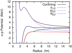
Figure 3: (Color online) The original and confining potentials for the $s_{1/2}$, $p_{3/2}$ and $d_{5/2}$ channels in the $\alpha-p$ subsystem. $R_{b}$ in Eqs. (24) and (25) is taken to be 5.7 fm for all the channels.

6Be ($ct=0$)

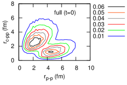
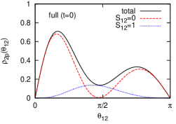
Figure 4: (Color online) The left panel: The 2p-density at $t=0$ obtained by including all the configurations up to $(h_{11/2})^{2}$. It is plotted as a function of $r_{\rm p-p}=(r_{1}^{2}+r_{2}^{2}-2r_{1}r_{2}\cos\theta_{12})^{1/2}$ and $r_{\rm c-pp}=(r_{1}^{2}+r_{2}^{2}+2r_{1}r_{2}\cos\theta_{12})^{1/2}/2$. The right panel: The angular distributions at $t=0$ obtained by integrating $\bar{\rho}_{2p}$ with respect to $r_{1}$ and $r_{2}$.

6Be ($ct=0$), $(l=odd)^{2}$ only

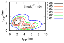
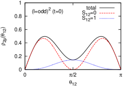
Figure 5: (Color online) The same as Fig. 4 but in the case with only odd-$l$ partial waves.

We generate the confining potential for the present problem as follows. Because the $\alpha$-p subsystem has a resonance at $E_{0}=1.96$ MeV in the $p_{3/2}$-channel, the two protons in ⁶Be are expected to have a large component of the $(p_{3/2})^{2}$ configuration. Thus, we first modify the core-proton potential for the $p_{3/2}$-channel in order to generate a bound state as follows:

$$V_{{\rm cp}}^{conf}(r) = V_{{\rm cp}}(r)\phantom{000}(r\leq R_{b}),$$ (24)

$$= V_{{\rm cp}}(R_{b})\phantom{00}(r>R_{b}),$$

with $R_{b}=5.7$ fm. Here we have followed Ref. 04Gurv and taken $R_{b}$ to be outside the potential barrier rather than the barrier position. For the other s.p. channels, we define the confining potential as

$$V_{\rm cp}^{conf}(r)=\left\{\begin{array}[]{cc}V_{\rm cp}(r)\phantom{0000}&(r\leq R_{b}),\\ V_{\rm cp}(r)+\Delta V_{p_{3/2}}(r)&(r>R_{b}),\end{array}\right.$$ (25)

where $\Delta V_{p_{3/2}}(r)=V_{{\rm cp}}(R_{b})-V_{{\rm cp}}(r)$ for the $p_{3/2}$-channel. The original and confining potentials for the $s_{1/2}$, $p_{3/2}$ and $d_{5/2}$ channels are shown in Fig. 3. We note that, for this system, the core-proton barrier is mainly due to the centrifugal potential rather than the Coulomb potential. This situation is quite different from heavy 2p-emitters with a large proton-number, such as ⁴⁵Fe.

⁶He (g.s.)

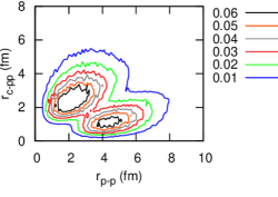
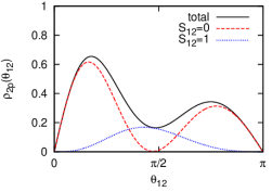
Figure 6: (Color online) The density distribution of the valence two neutrons, $\bar{\rho}_{2n}$, in the ground state of ⁶He. Those are plotted in the same manner as in the left and right panels of Fig. 4. The configurations up to $(h_{11/2})^{2}$ are included.

The initial state for the 2p-emission is obtained by diagonalizing the modified Hamiltonian including $V^{conf}_{\rm cp}(r)$. The empirical Q-value for the two-proton emission is 1.37 MeV for ⁶Be 88Ajz ; 02Till . However, the Minnesota potential with the original parameters overestimates this value by about 50%. Thus we have modified the parameter $v_{0}$ in Eq.(6) from the original value, $v_{0}=200.0$ MeV 77Thom , to $v_{0}=156.0$ MeV so as to yield $Q=1.37$ MeV when it is calculated by Eq.(16).

In Fig. 4, we show the density distribution of the initial state obtained in this way. By integrating the spin coordinates, the density distribution becomes a function of the radial distances, $r_{1}$ and $r_{2}$, as well as the opening angle between the two valence protons, $\theta_{12}$. That is,

$$\bar{\rho}_{2p}(t=0;r_{1},r_{2},\theta_{12})$$

$$\phantom{000}\equiv 8\pi^{2}r_{1}^{2}r_{2}^{2}\sin\theta_{12}\cdot\rho_{2p}(t=0;r_{1},r_{2},\theta_{12}),$$ (26)

with

$$\rho_{2p}(t=0;r_{1},r_{2},\theta_{12})=\left|\Psi(t=0;r_{1},r_{2},\theta_{12})\right|^{2}.$$ (27)

Here $\bar{\rho}_{2p}$ is normalized as

$$\int_{0}^{R_{\rm box}}dr_{1}\int_{0}^{R_{\rm box}}dr_{2}\int_{0}^{\pi}d\theta_{12}\,\bar{\rho}_{2p}=1.$$ (28)

In the left panel of Fig. 4, $\bar{\rho}_{2p}$ is plotted as a function of the distance between the core and the center of mass of the two protons: $r_{\rm c-pp}=\sqrt{r_{1}^{2}+r_{2}^{2}+2r_{1}r_{2}\cos\theta_{12}}/2$, and the relative distance between the two protons: $r_{\rm p-p}=\sqrt{r_{1}^{2}+r_{2}^{2}-2r_{1}r_{2}\cos\theta_{12}}$. In the right panel of Fig. 4, we also display the angular distributions obtained by integrating $\bar{\rho}_{2p}$ for the radial distances.

It is clearly seen that the initial wave function is confined inside the potential barrier at $r\cong 4$ fm (see Fig. 3). Furthermore, the 2p-density is concentrated near $r_{\rm p-p}=2$ fm, corresponding to the diproton correlation in bound nuclei 10Ois . The corresponding angular distribution becomes asymmetric and has the higher peak at the opening angle $\theta_{12}\cong\pi/6$. This peak is almost due to the spin-singlet configuration, being analogous to the dinucleon correlation. This suggests the existence of the diproton correlation in the meta-stable ground state of ⁶Be due to the pairing correlation.

As is well known, the mixture of configurations with s.p. states with opposite parity plays an essential role in generating the dinucleon correlation 84Catara . In order to study the effect of the diproton correlation in the 2p-emission, we have also performed the same calculation but only with odd-$l$ partial waves, that is, $p^{2},f^{2}$, and $h^{2}$. In the following, we call this case as the $(l=odd)^{2}$ case. In this case, the pairing correlations are taken into account only among the s.p. states with the same parity, while the mixture of opposite parity configurations is entirely ignored. In Fig. 5, we show the initial configuration obtained only with the odd-$l$ partial waves. We have used $v_{0}=88.98$ MeV in order to reproduce the empirical Q-value in this case. In the left panel of Fig. 5, there are two comparable peaks at $r_{\rm p-p}=2$ and $5$ fm whereas, in the right panel, the corresponding angular distribution has a symmetric form. This result is in contrast with that in the case with all the configurations from $(s_{1/2})^{2}$ to $(h_{11/2})^{2}$, shown in Fig. 4, where the pairing correlations are fully taken into account.

		6Be ($t=0$)			6He (g.s.)
		full	$(l=odd)^{2}$		full
$\Braket{H_{\rm 3b}}$ (MeV)		1.37	1.37		$-0.975$
$(p_{3/2})^{2}$ (%)		88.9	97.1		92.7
$(p_{1/2})^{2}$ (%)		03.1	02.8		01.6
$(s_{1/2})^{2}$ (%)		02.2	00.0		01.3
other $(l=even)^{2}$ (%)		05.2	00.0		04.2
other $(l=odd)^{2}$ (%)		00.6	00.1		00.2
$P(S=0)$ (%)		82.2	80.6		78.1

Table 2: Calculated properties for the initial state of ⁶Be and the bound ground state of ⁶He. The results with all the configurations from $(s_{1/2})^{2}$ to $(h_{11/2})^{2}$ are labeled by “full”. Those obtained only with the odd-$l$ partial waves for ⁶Be are also shown.

In Table 2, properties of the initial state are summarized. It is clearly seen that, in the case of the full configuration-mixture, the main component is $(p_{3/2})^{2}$, reflecting the fact that the $p_{3/2}$ channel has a resonance in the $\alpha$-p subsystem. The mixture of different partial waves are due to the off-diagonal matrix elements of $H_{\rm 3b}$, corresponding to the pairing correlations. A comparable enhancement of the spin-singlet configuration exists also in the case with the $(l=odd)^{2}$ bases, even though there is no localization of the two protons as shown in Fig. 5.

From the point of view of the isobaric symmetry in nuclei, it is interesting to compare the initial state of ⁶Be with the ground state of its mirror nucleus, ⁶He. Assuming the $\alpha$+n+n structure, we perform the similar calculation for the ground state of ⁶He. For the $\alpha$-n system, there is an observed resonance of $p_{3/2}$ at $E_{r}=0.735(20)$ MeV with its width, $\Gamma_{r}=0.600(20)$ MeV 88Ajz ; NNDCHP . In order to reproduce this resonance, we exclude the Coulomb term from $V_{\rm cp}$ and modify the depth parameter to $V_{0}=-61.25$ MeV in the Woods-Saxon potential. The pairing interaction is adjusted to reproduce the empirical two-neutron separation energy, $\Braket{H_{\rm 3b}}=-S_{\rm 2n}=-0.975$ MeV NNDCHP , by using $v_{0}=212.2$ MeV in Eq.(6). Notice that we deal with the bound state of the three-body system in this case, and thus the confining potential is not necessary. In Fig. 6, the two-neutron density distribution is shown in the same manner as in Fig. 4. Its properties are also summarized in the last column of Table 2. Obviously, the two-neutron wave function in ⁶He has a similar distribution to the 2p-wave function in ⁶Be. The dinucleon correlation is present also in ⁶He, characterized as the spatial localization with the enhanced spin-singlet component 05Hagi . Consequently, the confining potential which we employ provides such initial state of ⁶Be that can be interpreted as the isobaric analogue state of ⁶He.

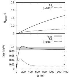
Figure 7: The decay probability and the decay width of the 2p-emission from ⁶Be, obtained with the time-dependent method. The result in the case of the full configuration-mixture is plotted by the solid line, whereas that in the $(l=odd)^{2}$ case is plotted by the dashed line. The experimental value, $\Gamma_{\rm exp}=92\pm 6$ keV 88Ajz ; 02Till , is marked by the shaded area.

III.2 Decay Width

In order to describe the decay process of ⁶Be, we suddenly change the potential at $t=0$ from the confining potential, $V_{\rm cp}^{conf}$, to the original one, $V_{\rm cp}$. The initial state constructed in the previous subsection then evolves in time. We first show the results of the decay probability, $N_{d}(t)$, and the decay width, $\Gamma(t)$, defined by Eqs.(18) and (19), respectively.

In Fig. 7, the calculation is carried out up to $ct=1400$ fm. We have confirmed that the artifact due to the reflection at $r=R_{\rm box}$ is negligible in this time-interval. One can clearly see that, after a sufficient time-evolution, the decay width converges to a constant value for all the cases, and the exponential decay-rule is realized. Furthermore, the result in the case of full configuration-mixture yields the saturated value of $\Gamma(t)\cong 88.2$ keV, which reproduces the experimental decay width, $\Gamma=92\pm 6$ keV 88Ajz ; 02Till .

On the other hand, the decay width is significantly underestimated when the partial waves are limited only to odd-$l$ partial waves (Note that we exclude even-$l$ partial waves not only at $t=0$ but also for $t>0$ in this case). The underestimation of the decay width is caused by an increase of the pairing attraction: with the odd-$l$ partial waves only, to reproduce the empirical Q-value, we needed a stronger pairing attraction. The two protons are then strongly bound to each other and are difficult to go outside, even they have a similar energy release to that in the case of full configuration-mixture. From this result, we can conclude that the mixing of opposite parity configurations is indispensable in order to reproduce simultaneously the Q-value and the decay width of the 2p-emission, supporting the assumption of the diproton correlation.

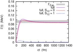
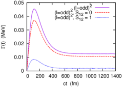
Figure 8: (Color online) The partial decay widths of the spin-singlet and the spin-triplet configurations in the 2p-emission of ⁶Be. In the upper panel, the result obtained with all the configurations from $(s_{1/2})^{2}$ to $(h_{11/2})^{2}$ is shown. In the lower panel, the same result but in the case with only odd-$l$ partial waves is plotted.

	$\Gamma_{\rm tot}$ (keV)	$\Gamma_{S=0}$ (keV)	$\Gamma_{S=1}$ (keV)
full	088.2	087.1	001.1
$(l=odd)^{2}$ only	012.5	010.7	001.8
no-pairing	348.0	232.0	116.0
($ct=3000$ fm)

Table 3: The contributions from the spin-singlet and the spin-triplet configurations to the total decay width. Note that the experimental value of the total decay width is $92\pm 6$ keV 88Ajz ; 02Till . All the values are evaluated at $ct=1200$ fm, except those in the “no-pairing” case, which are evaluated at $ct=3000$ fm. In all the cases, the total energy release (Q-value) of the two protons is set to be consistent to the experimental value, $1.37$ MeV.

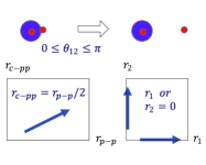
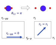
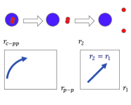
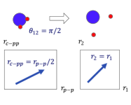
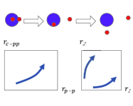
(a) diproton (d) one-proton (b) simultaneous, $\theta_{12}=0$ (e) correlated (c) simultaneous, $\theta_{12}=\pi/2$ (f) sequential

Figure 9: (Color online) (a)-(c): Schematic illustrations for the trajectories of different 2p-emission modes. (d): The trajectory of the $1p$-emission. (e),(f): The same as the panels (a)-(d) but of the hybrid 2p-emissions. See the main text for the details.

For the above two cases, we also calculate the partial decay widths for the spin-singlet and the spin-triplet configurations. The corresponding formula to Eq.(23) is given as

$$\Gamma_{S}(t)\equiv\frac{\hbar}{1-N_{d}(t)}\frac{d}{dt}N_{d,S}(t),$$ (29)

with

$$N_{d,S}(t)\equiv\Braket{\Psi_{d,S}(t)}{\Psi_{d,S}(t)}$$ (30)

$$=\int_{0}^{R_{\rm box}}dr_{1}\int_{0}^{R_{\rm box}}dr_{2}\int_{0}^{\pi}d\theta_{12}$$

$$\phantom{0000}\times 8\pi^{2}r_{1}^{2}r_{2}^{2}\sin\theta_{12}\left|\Psi_{d,S}(t;r_{1},r_{2},\theta_{12})\right|^{2}.$$ (31)

where $S$ indicates the combined spin of the two protons. The results are shown in Fig. 8. Clearly, the spin-singlet configuration almost exhausts the decay width in the case of full configuration-mixture shown in the upper panel of Fig. 8. This suggests that the emitted two protons from the ground state of ⁶Be have mostly the $S=0$ configuration like a diproton. On the other hand, in the lower panel of Fig. 8, one can see that the spin-triplet configuration occupies a considerable amount of the total decay width when we exclude even-$l$ partial waves.

In the first and the second rows of Table 3, we tabulate the total and partial widths in the case of full configuration-mixture and in the $(l=odd)^{2}$ cases, respectively. The values are evaluated at $ct=1200$ fm, where the total widths sufficiently converge. Clearly, there is a significant increase of the spin-singlet width in the case of full configuration-mixture, by about one order of magnitude larger than that in the case of $(l=odd)^{2}$ waves. On the other hand, we get similar values of the spin-triplet width in these two cases. From this result, we can conclude that the mixture of the odd-$l$ and even-$l$ s.p. states is responsible for the enhancement of the spin-singlet emission, although the dominance of the spin-singlet configuration in the initial state is apparent in both the two cases.

A qualitative reason for the dominance of the spin-singlet configuration is due to the $(s_{1/2})^{2}$ channel. Notice that the $(s_{1/2})^{2}$-channel is allowed only for $S=0$. Because there is no centrifugal barrier in this channel, the spin-singlet emission can be dominant. On the other hand, for the spin-triplet configuration, only $L=1$ is permitted. Thus the $(s_{1/2})^{2}$ configuration does not contribute to it, and there is a centrifugal barrier for all the channels in the spin-triplet configuration. Consequently, apart from the reduction due to the stronger pairing attraction, the spin-triplet widths are similar in both the two cases.

III.3 Time-Evolution of Decay State

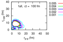
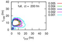
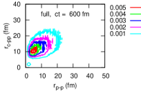
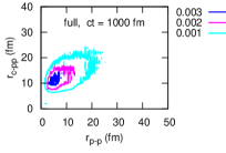
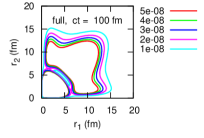
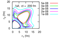
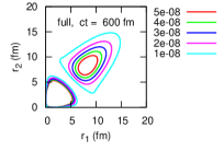
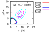
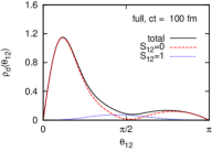
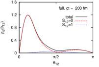
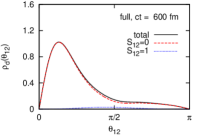
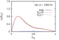
Figure 10: (Color online) The 2p-density distribution for the decay states, $\bar{\rho}_{d}(t)$, obtained with the time-dependent calculations. All the uncorrelated basis up to $(h_{11/2})^{2}$ are included. The left column: (i) the distribution as a function of $r_{\rm c-pp}$ and $r_{\rm p-p}$. The middle column: (ii) the distribution as a function of $r_{1}$ and $r_{2}$, obtained by integrating $\bar{\rho}_{d}$ for $\theta_{12}$. In order to clarify the peak(s), the radial weight $r_{1}^{2}r_{2}^{2}$ is omitted. The right column: (iii) the angular distribution of the decay state plotted as a function of the opening angle $\theta_{12}$ between the two protons. It is obtained by integrating $\bar{\rho}_{d}(t)$ for the radial coordinates, $r_{1}$ and $r_{2}$. Beside the total distribution, the spin-singlet and spin-triplet components are also plotted.

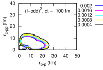
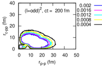
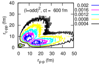
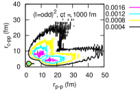
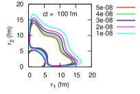
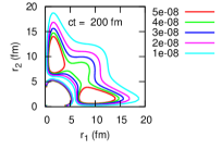
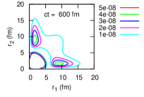
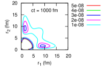
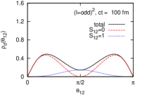
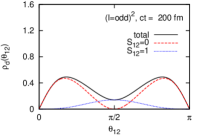
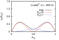
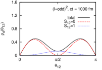
Figure 11: (Color online) The same as Fig.10 but for the case with only $(l=odd)^{2}$ waves. Notice a different scale in the left column from that in Fig.10.

In order to discuss the dynamics of the emission process, we show the density distribution of the decay state,

$$\bar{\rho}_{d}(t)=8\pi^{2}r_{1}^{2}r_{2}^{2}\sin\theta_{12}\rho_{d}(t),$$ (32)

$$\rho_{d}(t)=\left|\Psi_{d}(t;r_{1},r_{2},\theta_{12})\right|^{2}.$$ (33)

The decay state, which is orthogonal to the initial state confined inside the potential barrier, has the most of its amplitude outside the potential barrier. In the following, we adopt three sets of radial coordinates: (i) The first set includes $r_{\rm c-pp}$ and $r_{\rm p-p}$, similarly to the left panel of Fig. 4. (ii) In the second set, we integrate $\bar{\rho}_{d}$ with respect to the opening angle, $\theta_{12}$, and plot it as a function of $r_{1}$ and $r_{2}$. In order to see the peak-structure clearly, we omit the radial weight $r_{1}^{2}r_{2}^{2}$ in $\bar{\rho}_{d}$ in the second set. (iii) Within the third set, on the other hand, we integrate $\bar{\rho}_{d}(t)$ over the radial distances, and plot it as a function of $\theta_{12}$. We will use in Figs. 10, 11 and 13 these sets of coordinates in order to present the amplitude of the decay state in actual calculations.

Before we show the results of the actual calculations, we schematically illustrate the dynamic of the 2p-emissions in Fig. 9. From the geometry, the emission modes are classified into two categories: “simultaneous two-proton” and “one-proton” emissions. The diproton emission is a special case of the first category. The second category corresponds to the case where only one proton penetrates the barrier.

Figs. 9(a), (b) and (c) correspond to the simultaneous 2p-emissions with $\theta_{12}=0,\pi$ and $\pi/2$, respectively, where $\theta_{12}=0$ (Fig.9(a)) corresponds to the diproton emission. In these three cases, the density in the $(r_{1},r_{2})$-plane shows the same patterns, and is concentrated along $r_{1}\cong r_{2}$. The simultaneous emissions with different opening angles can be distinguished only in the $(r_{\rm p-p},r_{\rm c-pp})$-plane: for instance, in the diproton emission, the probability shows mainly along the line with $r_{\rm c-pp}\gg r_{\rm p-p}$, while it is along the line with $r_{\rm c-pp}=0$ for $\theta_{12}=\pi$. In the one-proton emission shown in Fig.9(d), only one of the two protons goes through the barrier while the other proton remains inside the core nucleus. This is seen as the increment along $r_{\rm c-pp}\cong r_{\rm p-p}/2$ and $r_{1}$ or $r_{2}\cong 0$ lines.

In Fig. 9(e) and (f), we illustrate two hybrid processes. The first one is a “correlated emission”, shown in Fig. 9(e). In the correlated emission, the two protons are emitted simultaneously to almost the same direction, holding the diproton-like configuration. In this mode, in the early stage of tunneling, the density distribution has a larger amplitude in the region with $r_{1}\cong r_{2}$ and small $\theta_{12}$. In the $(r_{\rm p-p},r_{\rm c-pp})$-plane, it corresponds to the increment of the probability in the region of $r_{\rm p-p}\ll r_{\rm c-pp}$. After the barrier penetration, the two protons separate from each other mainly due to the Coulomb repulsion. The second hybrid process is a “sequential emission”, which is shown in Fig. 9(f). In this mode, there is a large possibility in which one proton is emitted whereas the other proton remains around the core. The density distribution shows high peaks along $r_{1}\gg r_{2}$ and $r_{1}\ll r_{2}$. In the $(r_{\rm p-p},r_{\rm c-pp})$-plane, it corresponds to the increment along the line of $r_{\rm c-pp}\cong r_{\rm p-p}/2$. In contrast to the pure one-proton emission, the remaining proton eventually goes through the barrier when the core-proton subsystem is unbound.

III.3.1 case of full configuration-mixture

We now show the results of the time-dependent calculations for the 2p-emission of ⁶Be. We first discuss the case of full configuration-mixture, where the odd-$l$ and even-$l$ single particle states are fully mixed by the pairing correlation. The density distribution for the decay state along the time-evolution is shown in Fig. 10. The left, middle and right columns correspond to the coordinate sets (i), (ii) and (iii) defined before, respectively. The first to the fourth panels in each column show the decay-density at $ct=100,200,600$ and $1000$ fm, respectively. For a presentation purpose, we normalize $\bar{\rho}_{d}$ at each step of time.

In the left and middle columns of Fig. 10, it can be seen that the process in this case is likely the correlated emission shown in Fig. 9(e). Contributions from the other modes shown in Fig. 9 are small. In the middle column of Fig. 10, during the time-evolution, there is a significant increment of $\bar{\rho}_{d}$ along the line with $r_{1}\cong r_{2}$. The corresponding peak in the left column is at $r_{\rm p-p}\ll r_{\rm c-pp}\cong 10$ fm, which means a small value of $\theta_{12}$. It should also be noted that, after the barrier penetration, the two protons lose their diproton-like configuration due to the Coulomb repulsion, which results in the increase of $r_{\rm p-p}$. Thus, for $r_{\rm c-pp}\geq 10$ fm which is a typical position of the potential barrier from the core, the density distribution extends around the $r_{\rm c-pp}\cong r_{\rm p-p}$ region. In this process, the pairing correlation plays an important role to generate the significant diproton-like configuration before the end of the barrier penetration. In the right column of Fig. 10, the distributions are also displayed as a function of the opening angle, $\theta_{12}$. We can clearly see that the decay state has a high peak at $\theta_{12}\cong\pi/6$ in this time-region.

These results imply that the two protons are emitted almost in the same direction, at least in the early stage of the emission process. Intuitively, from the uncertainty principle, this would correspond to a large opening angle in the momentum space. Indeed, such component has been experimentally observed to be dominant for the 2p-decay of ⁶Be 09Gri_80 ; 09Gri_677 . It would be an interesting future work to carry out the Fourier transformation of the decay state and compare our calculations with the experimental data.

III.3.2 $(l=odd)^{2}$ case

We next discuss the case only with $(l=odd)^{2}$ bases. In Fig. 11, the decay density shows a strong pattern of the sequential emission demonstrated in Fig. 9(f): significant increments occur along the lines with $r_{\rm c-pp}\cong r_{\rm p-p}/2$ and $r_{1}\gg r_{2}$ or $r_{1}\ll r_{2}$. Notice that the contribution from the simultaneous emissions also exists, especially in the early time-region. As a result, the decay state has widely spread amplitudes as a mixture of these emission modes. However, the simultaneous mode is minor compared with the case of full configuration-mixture. Notice that the condition for a true 2p-emitter is satisfied also in this case: the core-proton resonance is located at $1.96$ MeV which is above $Q_{\rm 2p}=1.37$ MeV. However, even with the strong pairing attraction and the energy condition for the true 2p-emitter, the process hardly becomes the correlated emission when the parity-mixing is forbidden or extensively suppressed. The angular distribution shows exactly the symmetric form, and is almost invariant during the time-evolution. This is because we exclude the pairing correlation between the positive and negative parity states in the core-proton system, not only at $t=0$ but also during the time-evolution.

III.3.3 no-pairing case

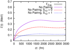
Figure 12: (Color online) The same as Fig. 8 but for the case without pairing correlations.

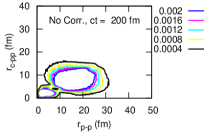
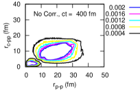
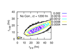
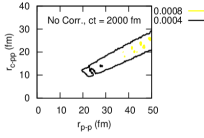
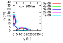
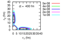
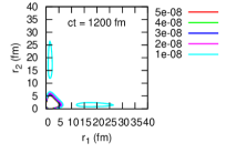
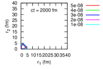
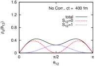
Figure 13: (Color online) The same as Fig. 10 but for the case without pairing correlations.

Finally, for a comparison with the above two cases, we also perform similar calculations but by completely neglecting the pairing correlation. In this case, we only consider the uncorrelated Hamiltonian, $h_{1}+h_{2}$. Because of the absence of the non-diagonal components in the Hamiltonian matrix, it can be proved that, if the s.p. resonance is at an energy $\epsilon_{0}$ with its width $\gamma_{0}$, the 2p-resonance is at $2\epsilon_{0}$ with its width $2\gamma_{0}$. The 2p-wave function is expanded on the uncorrelated basis with a single set of angular quantum numbers. Namely,

$$\ket{\Psi_{(lj)}(t)}=\sum_{n_{a},n_{b}}C_{n_{a}n_{b}}(t)\ket{{\Phi}_{n_{a}n_{b}lj}},$$ (34)

where $(lj)=p_{3/2}$ for ⁶Be. In order to reproduce the empirical Q-value of ⁶Be, we inevitably modify the core-proton potential. We employ $V_{0}=-68.65$ MeV to yield the s.p. resonance at $\epsilon_{0}(p_{3/2})=1.37/2=0.685$ MeV, although the scattering data for the core-proton subsystem are not reproduced and the character of a true 2p-emitter disappears. With this potential, we obtain the s.p. resonance with a broad width: $\gamma_{0}(p_{3/2})\cong 170$ keV. Because of the broad decay width, we need to increase the radial box to $R_{\rm box}=200$ fm in order to neglect the artifact due to the reflection at $R_{\rm box}$ in the long time-evolution.

The result for the decay width is shown in Fig. 12 and in the last row of Table 3. To get the saturated result, we somewhat need a relatively longer time-evolution than that in the case of full configuration-mixture. Thus, in Table 3, we evaluate the decay width at $ct=3000$ fm. By this time, the total decay width, $\Gamma(t)$, converges to about $340$ keV which is consistent to that expected from the s.p. resonance, $\gamma_{0}(p_{3/2})$. During the time-interval shown in Fig. 12, there still remain some oscillations in $\Gamma(t)$. This is a characteristic behavior of the broad resonance, namely an oscillatory deviation from the exponential decay-rule. For the spin-singlet and triplet configurations, their contributions have exactly the ratio of $2:1$. This result is simply due to the re-coupling of the angular momentum for the $(p_{3/2})^{2}$ configuration.

By comparing these results with those in the case of the full configuration-mixing, we can clearly see a decisive role of the pairing correlations in 2p-emissions. Assuming the empirical Q-value, if we explicitly consider the pairing correlations, the decay width becomes narrow and agrees with the experimental data. On the other hand, in the no-pairing case, we need a modified core-proton interaction to reproduce the empirical Q-value, and the properties of the core-proton resonance state become inconsistent with the experimental data. Even though the Q-value is adjusted in this way, the calculated 2p-decay width is significantly overestimated in this case. Namely, we cannot simultaneously reproduce the experimental Q-value and the decay width with the no-pairing assumption. If one is forced to reproduce them simultaneously, one may need an unphysical core-proton interactions.

In Fig. 13, we show the density distribution of the decay state during the time-evolution. Obviously, in this case, the process is the sequential or, moreover, like the one-proton emission. There is a significant increase of the density along the lines with $r_{\rm c-pp}\cong r_{\rm p-p}/2$ and, consistently, with $r_{1}\gg r_{2}$ and $r_{1}\ll r_{2}$ (see Fig. 9). On the other hand, the probability for the simultaneous and correlated emissions are negligibly small. This is quite different from that in the case of full configuration-mixture, where the correlated emission is apparent.

III.4 Role of Pairing Correlation in Decay Width

In this subsection, we discuss a general role of the pairing correlation in the 2p-emission. To this end, we calculate the 2p-decay width for different Q-values in the case of full configuration-mixture and the no-pairing case. The variation of the Q-value is done by changing the parameter $V_{0}$ in the core-proton potential (Eq.(4)), while the pairing interaction used in the case of full configuration mixture is kept unchanged. Notice that for the no-pairing case, the s.p. resonance appears at $\epsilon_{0}(p_{3/2})=Q/2$.

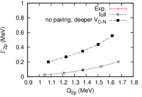
Figure 14: The calculated decay width for the 2p-emission of ⁶Be, as a function of the Q-value. The Q-value is varied by modifying the core-proton potential. The experimental values, $Q_{\rm 2p}=1.372(5)$ MeV and $\Gamma_{\rm 2p}=0.092(6)$ MeV NNDCHP , are also indicated.

In Fig. 14, the decay width is plotted as a function of the decay Q-value. We note that the calculated decay widths are well converged after a sufficient time-evolution in all the cases. The decay width is evaluated at $ct=1200$ and $3000$ fm in the full-correlation and the no-pairing cases, respectively. Clearly, the no-pairing calculations overestimate the decay width, in all the region of $Q_{\rm 2p}$. Namely, the three-body system becomes easier to decay without the pairing correlation, for the same value of the total energy release (Q-value). In other words, the pairing correlation plays an essential role in the meta-stable state, stabilizing it against particle emissions. We note that a similar effect has been predicted also for a one-neutron resonance, that is, the width of a one-neutron resonance becomes narrow when one considers the pairing correlations 14Kobayashi .

Also, as we have confirmed in the previous section, the emission dynamics with and without the pairing correlations are essentially different to each other: the correlated emission becomes dominant if the pairing correlation is fully considered, whereas the sequential emission plays a major role in the no-pairing case. Consequently, the pairing correlation must be treated explicitly in the meta-stable states, otherwise one would miss the essential effect on both the decay-rule and the dynamical phenomena.

IV Summary

We have investigated the 2p-emission of the ⁶Be nucleus by employing a three-body model consisting of an $\alpha$ particle and two valence protons. We have applied the time-dependent method and discussed the decay dynamics of many-body meta-stale states, particularly in connection to the diproton correlation. An advantage of the time-dependent method is that it provides not only a way to evaluate the decay width, but also an intuitive way to understand the decay dynamics.

By using the confining potential method, we first obtained the initial state of ⁶Be, in which the two protons are confined inside the potential barrier. Because of the pairing correlation between the two protons, the initial configuration includes the diproton correlation, similarly to the dineutron correlation in the ground states of Borromean nuclei such as ⁶He. At time $t=0$, the confinement is removed so that the 2p-state evolves in space and time. In this calculation, the decay width can be read off by plotting the survival probability as a function of time. We have found that our Hamiltonian well reproduces simultaneously the experimental Q-value and decay width of ⁶Be. We have also shown that the decay state predominantly has the spin-singlet configuration.

By monitoring the time-evolution of the density distribution of the decay state, we have confirmed that the decay process in the early stage is mainly the correlated emission, in which the two protons tend to be emitted in a similar direction, reflecting the diproton correlation in the initial state. Thus, the 2p-emission can be a promising tool to probe experimentally the diproton correlation. We have also performed the calculations by including only odd-$l$ partial waves in order to switch off the diproton correlation. In this case, even though we use the model parameters which reproduce the empirical Q-value, the decay width is significantly underestimated. The decay process shows a large component of the sequential emission, in contrast to the case of full configuration-mixture. From these results, we can conclude that the diproton correlation plays an important role in the 2p-emission, providing an opportunity to probe it by observing the 2p-emission.

We have also checked that, if the pairing correlation is completely neglected, the decay width is largely overestimated, partly because the proton-core potential has to be made deeper in order to yield the empirical Q-value. By monitoring the time-evolution of the density distribution of the decay state, it has been clarified that the emission is mostly a sequential decay with the no-pairing assumption. Namely, the pairing correlation is critically important to determine not only the decay width but also the dynamical phenomena.

In order to compare quantitatively the calculated results with the experimental data, we would need a more careful treatment of the final-state interactions (FSIs). In this work, we mainly treat the early stage of the time-evolution, terminating the calculations at $ct\sim 1400$ fm in order to avoid the artifact due to the reflection at the edge of the box, $R_{\rm box}$. On the other hand, the two protons are detected in the actual experiments at a much later time after being significantly affected by the FSIs. In order to fully take into account the FSIs, we would have to use an extremely large box even though the computational costs would increase severely.

The time-dependent method which we employed in this paper can be applied also to a decay of other many-body meta-stable states. It provides a novel and intuitive point of view to the decay process. It would be an interesting future problem to apply this method to other problems of many-particle quantum decays, such as the two-neutron emission and the two-electron auto-ionization of atoms.

- (1) D. M. Brink and R. A. Broglia, “Nuclear Superfluidity” (Cambridge University Press, Cambridge, 2005).
- (2) P. Ring and P. Schuck, The Nuclear Many Body Problem (Springer-Verlag, New York, 1980).
- (3) Fifty Years of Nuclear BCS: Pairing in Finite Systems, edited by R.A. Broglia and V. Zelevinsky (World Scientific, Singapore, 2013).
- (4) J. Dobaczewski et al., Phys. Rev. C 53, 2809 (1996).
- (5) D. J. Dean and M. Hjorth-Jensen, Rev. Mod. Phys. 75, 607 (2003).
- (6) A.B. Migdal, Sov. J. of Phys. 16, 238 (1973).
- (7) F. Catara, A. Insolia, E. Maglione and A. Vitturi, Phys. Rev. C 29 1091 (1984).
- (8) G.F. Bertsch and H. Esbensen, Ann. Phys. (NY) 209, 327 (1991).
- (9) M.V. Zhukov et al., Phys. Rep. 231, 151 (1993).
- (10) Yu. Ts. Oganessian, V.I. Zagrebaev, and J.S. Vaagen, Phys. Rev. Lett. 82, 4996 (1999); Phys. Rev. C60, 044605 (1999).
- (11) M. Matsuo, K. Mizuyama and Y. Serizawa, Phys. Rev. C 71, 064326 (2005).
- (12) M. Matsuo, Phys. Rev. C 73, 044309 (2006).
- (13) K. Hagino and H. Sagawa, Phys. Rev. C 72, 044321 (2005).
- (14) T. Oishi, K. Hagino and H. Sagawa, Phys. Rev. C 82, 024315 (2010).
- (15) N. Pillet, N. Sandulescu, P. Schuck, and J.-F. Berger, Phys. Rev. C81, 034307 (2010).
- (16) L.G. Cao, U. Lombardo, and P. Schuck, Phys. Rev. C74, 064301 (2006).
- (17) J. Margueron, H. Sagawa, and K. Hagino, Phys. Rev. C 76, 064316 (2007).
- (18) K. Hagino, H. Sagawa, J. Carbonell, and P. Schuck, Phys. Rev. Lett. 99, 022506 (2007).
- (19) M. Igarashi, K. Kubo and K. Yagi, Physics Reports 199 1 (1991).
- (20) W. von Oertzen and A. Vitturi, Reports on Progress in Physics 64 1247 (2001).
- (21) H. Shimoyama and M. Matsuo, Phys. Rev. C 84 044317 (2011).
- (22) N. Fukuda et al., Phys. Rev. C 70, 054606 (2004).
- (23) T. Nakamura et al., Phys. Rev. Lett. 96, 252502 (2006).
- (24) T. Myo et al., Phys. Rev. C 63, 054313 (2001).
- (25) K. Hagino and H. Sagawa, Phys. Rev. C 76, 047302 (2007).
- (26) C. A. Bertulani and M. S. Hussein, Phys. Rev. C 76, 051602(R) (2007).
- (27) T. Oishi, K. Hagino and H. Sagawa, Phys. Rev. C 84, 057301 (2011).
- (28) Yuma Kikuchi et al., Phys. Rev. C 81, 044308 (2010).
- (29) B. Blank and M. Ploszajczak, Rep. Prog. Phys. 71, 046301 (2008).
- (30) M. Pfützner, et al., Rev. Mod. Phys. 84, 567-619 (2012).
- (31) L. V. Grigorenko, Physics of Particles and Nuclei 40, 674 (2009).
- (32) V.V. Flambaum and V.G. Zelevinsky, J. Phys. G 31, 335 (2005).
- (33) C.A. Bertulani, V.V. Flambaum and V.G. Zelevinsky, J. Phys. G 34, 2289 (2007).
- (34) C.A. Bertulani, M.S. Hussein, and G. Verde, Phys. Lett. B 666, 86 (2008).
- (35) T. Maruyama, T. Oishi, K. Hagino and H. Sagawa, Phys. Rev. C 86, 044301 (2012).
- (36) V.I. Goldansky, Nucl. Phys. 19, 482-495 (1960).
- (37) V.I. Goldansky, Nucl. Phys. 27, 648-664 (1961).
- (38) D.S. Delion, R.J. Liotta and R. Wyss, Phys. Rev. C 87, 034328 (2013).
- (39) O.V. Bochkarev et al., Nucl. Phys. A 505, 215 (1989).
- (40) L. V. Grigorenko et al., Phys. Rev. C80, 034602 (2009).
- (41) L. V. Grigorenko et al., Phys. Lett. B 677, 30-35 (2009).
- (42) I.A. Egorova et al., Phys. Rev. Lett. 109, 202502 (2012).
- (43) L.V. Grigorenko et al., Phys. Rev. C 86, 061602(R) (2012).
- (44) J. Rotureau, J. Okolowicz and M. Ploszajczak, Phys. Rev. Lett. 95, 042503 (2005).
- (45) K. Miernik et al., Phys. Rev. Lett. 99, 192501 (2007).
- (46) I. Mukha et al., Phys Rev. C 77, 061303(R) (2008).
- (47) I. Mukha et al., Phys Rev. C 82, 054315 (2010).
- (48) A. Bohm, M. Gadella and G. Bruce Mainland, American J. of Phys. 57, 1103-1108 (1989).
- (49) G.A. Gamov, Z. Phys. 51, 204-212 (1928) ; Z. Phys. 52, 510-515 (1928).
- (50) R.W. Gurney and E.U. Condon, Phys. Rev. 33, 127-140 (1929).
- (51) N.S. Krylov and V.A. Fock, Zh. Éksp. Teor. Fiz. 17, 93 (1947).
- (52) V.I. Kukulin, V.M. Krasnopolśky and J. Horác̆ek, “Theory of Resonances” (Kluwer Achademic Publishers, 1989).
- (53) L.V. Grigorenko et al., Phys. Rev. C 64, 054002 (2001).
- (54) S. Åberg, P.B. Semmes and W. Nazarewicz, Phys. Rev. C 56, 1762 (1997).
- (55) C.N. Davis and H. Esbensen, Phys. Rev. C 61, 054302 (2000).
- (56) O. Serot, N. Carjan and D. Strottman, Nucl. Phys. A 569, 562 (1994).
- (57) P. Talou, N. Carjan and D. Strottman, Phys. Rev. C 58, 3280 (1998).
- (58) P. Talou, D. Strottman and N. Carjan, Phys. Rev. C 60, 054318 (1999).
- (59) P. Talou, N. Carjan, C. Negrevergne and D. Strottman, Phys. Rev. C 62, 014609 (2000).
- (60) G. García-Calderón and L.G. Mendoza-Luna, Phys. Rev. A 84, 032106 (2011).
- (61) A. del Campo, Phys. Rev. A 84, 012113 (2011).
- (62) M. Pons, D. Sokolovski and A. del Campo, phys. Rev. A 85, 022107 (2012).
- (63) F. Ajzenberg-Selove, Nucl. Phys. A 490, 1-225 (1988).
- (64) D.R. Tilley et al., Nucl. Phys. A 708, 3-163 (2002).
- (65) M. Hoefmann et al., Phys. Rev. Lett. 85, 1404-1407 (2000).
- (66) A.M. Shirokov et al., Phys. Rev. C 79, 014610 (2009).
- (67) E. Hairer, S.P. Nørsett and G. Wanner, “Solving Ordinary Differential Equations I” (Springer-Verlag, Berlin, 1993), and references there in.
- (68) D.R. Thompson, M. Lemere and Y.C. Tang, Nucl. Phys. A 286, 53-66 (1977).
- (69) S.A. Gurvitz and G. Kalbermann, Phys. Rev. Lett. 59, 262 (1987).
- (70) S.A. Gurvitz, Phys. Rev. A 38, 1747 (1988).
- (71) S.A. Gurvitz et al., Phys. Rev. A 69, 042705 (2004).
- (72) “Chart of Nclides”, Database of National Nuclear Data Center (NNDC), http://www.nndc.bnl.gov/chart/.
- (73) S. Aoyama, S. Mukai, K. Katō and K. Ikeda, Progress of Theoretical Physics 94, 343 (1995).
- (74) R. Kobayashi and M. Matsuo, private communications.