Projector augmented-wave and all-electron calculations across the periodic table:
a comparison of structural and energetic properties

Abstract

We construct a reference database of materials properties calculated using density-functional theory in the local or generalized-gradient approximation, and an all-electron or a projector augmented-wave (PAW) formulation, for verification and validation of first-principles simulations. All-electron calculations use the full-potential linearised augmented-plane wave method, as implemented in the Elk open-source code, while PAW calculations use the datasets developed by some of us in the open-source PSlibrary repository and the Quantum ESPRESSO distribution. We first calculate lattice parameters, bulk moduli, and energy differences for alkaline metals, alkaline earths, and $3d$ and $4d$ transition metals in three ideal, reference phases (simple cubic, fcc, and bcc), representing a standardized crystalline monoatomic solid-state test. Then, as suggested by K. Lejaeghere et al., [Critical Reviews in Solid State and Material Sciences 39, p 1 (2014)], we compare the equations of state for all elements, except lanthanides and actinides, in their experimental phase (or occasionally a simpler, closely related one). PAW and all-electron energy differences and structural parameters agree in most cases within a few meV/atom and a fraction of a percent, respectively. This level of agreement, comparable with the previous study, includes also other PAW and all-electron data from the electronic-structure codes VASP and WIEN2K, and underscores the overall reliability of current, state-of-the-art electronic-structure calculations. At the same time, discrepancies that arise even within the same formulation for simple, fundamental structural properties point to the urgent need of establishing standards for verification and validation, reference data sets, and careful refinements of the computational approaches used.

I Introduction

Density functional theory (DFT) electronic structure calculations within the plane-wave pseudopotential (PP) method are routinely used to study and predict the properties of materials as well as for gaining fundamental insights in quantum physics and chemistry. Many researchers use pseudopotentials to study increasingly complex systems with techniques requiring massive numerical efforts such as the many-body perturbation theory, time-dependent DFT, crystal structure search, metadynamics, high-throughput searches of material properties Onida2002 ; Martonak2006 ; Curtarolo2013 ; Jain2013 ; Marzari2006 .

The transferability of a PP depends on several factors and over the years many recipes have been proposed, starting from empirical methods and arriving to modern ab-initio approaches including norm conserving (NC) PPs, NC ultrasoft (US) PPs, US or the projector augmented-wave (PAW) method. Blochl1994 ; Kresse1999 The choice of PP parameters is far from straightforward and in many cases requires several refinements through extensive evaluations in which PPs are tested in different electronic environments. Moreover, a trade-off between accuracy and numerical efficiency must be made leading to PPs of different performance. Unfortunately, many pseudopotentials routinely used do not come with a standard set of tests and must be checked before use, since their accuracy is poorly documented or unknown. Moreover, standardized tests that could give an unbiased quantitative measure of the PP transferability are still missing, with users testing the quantity of interest by searching reference data in the literature or performing time-consuming all-electron calculations for comparison.

Some systematic efforts to obtain a unified, reliable, and accepted test procedure for PPs have started to appear in the literature. Standardized set of molecules, well established in the computational chemistry community (such as the so called G2-1 setCurtiss1991 ; Grossman2002 ; Nemec2010 ) have been used to compare PAW and all-electron localized basis set calculations. Paier2005 Recently, Lejaeghere et al. Lejaeghere2013 have used all-electron (WIEN2kWIEN2kweb ) and pseudopotential (GPAWGPAW and VASPVASPweb ) codes to define quantitatively the discrepancies in the equations of state fo a wide set of elemental solids in the periodic table (71 elements). In that study, the zero pressure stable phase was chosen as reference for most of the elements. More recently, the lattice constant, bulk moduli and energy differences of the face-centered and body-centered cubic structures of several elements have been used to assess the accuracy of a new set of US PPs by Garrity, Bennett, Rabe and Vanderbilt (GBVR), GBRV that introduced a library of PPs targeted at high-throughput calculations.

In the current study, we contribute to these validation and verification efforts by i) introducing a standardized crystalline monoatomic solid test (CMST) where each element is studied in several crystal structures, ii) providing our own all-electron CMST results using the Elk codeelkweb and iii) testing the PSlibrary pslibrary PAW datasets of the Quantum ESPRESSO (QE) distribution espresso with respect to Elk for CMST, and with respect to Elk, WIEN2k WIEN2kweb , and VASPVASPweb for the equilibrium structure proposed in Ref. Lejaeghere2013, .

The paper is organized as follows: In Section II we describe the methodology of the present study and the computational parameters used in our calculations, and we introduce the PSlibrary PAW datasets used for elements that have not been described elsewhere. In Section III.1 we validate our Elk all-electron results by comparing them, whenever possible to the results in the literature. Then, in Section III.2 Elk data are compared with the PSlibrary on the CMST. In section III.3 we follow the methodology of Ref. Lejaeghere2013, and extend these tests to a majority of the periodic table (68 elements). We provide additional Elk and QE results obtained using the PSlibrary distribution, which will be referred as QE-PAW hereon, to be compared with the previous data. Conclusions are given in section IV.

II Methodology

II.1 Crystalline Monoatomic Solid Test

We propose here to define a standardized crystalline monoatomic solid test, CMST, consisting of the study of each element in three crystal structures: simple cubic (sc), face-centered cubic (fcc), and body-centered cubic (bcc), focusing on the zero pressure equilibrium lattice constant and bulk modulus and on the energy differences among the three phases in non-magnetic configurations.

The lattice constant $a_{0}$, the bulk modulus $B_{0}$ and the total energy $E_{tot}$ at zero pressure are calculated fitting the total energy as a function of the volume. An energy-volume curve is calculated with $15$ points around a first estimate of $a_{0}$ (from -7% to +7%, in 1% steps), which is fitted with a third order Birch-Murnaghan equation of state (EoS),

$$\begin{split}E(V)=&E_{0}+\frac{9}{16}B_{0}V_{0}\left[\left(\frac{V_{0}}{V}\right)^{\frac{2}{3}}-1\right]^{2}\\ &\cdot\left\{2+\left[\left(\frac{V_{0}}{V}\right)^{\frac{2}{3}}-1\right]\left(B^{\prime}_{0}-4\right)\right\},\end{split}$$ (1)

where $E_{0}$ is the equilibrium total energy , $V_{0}$ is the equilibrium volume, and $B_{0}$ and $B^{\prime}_{0}$ are the bulk modulus and its pressure derivative, respectively.

This procedure is iterated until the new $a_{0}$ differs from the old one by less than $2\times 10^{-4}$ Å  ensuring that the EoS parameters are well converged and the initial information on the lattice constant does not bias the final results. The final EoS fits are then validated by comparing the total energies obtained through direct calculations at $a_{0}$ and the ones obtained from the EoS, which agree very well within 1 meV/atom.

For a few elements and a few values of the lattice parameter we have encountered convergence issues with Elk when the PBEPerdew1996 exchange-correlation was used, while no convergence issues were found in the LDAPerdew1981 calculations. In all cases the EoS fit could be carried out satisfactorily as at least 11 points were successfully completed. The list of elements and structures with convergence issues in PBE are reported in the Supplementary Material.

The CMST procedure was carried out for all elements in the alkaline metals, the alkaline earths, and the $3d$ and $4d$ transition metals series.

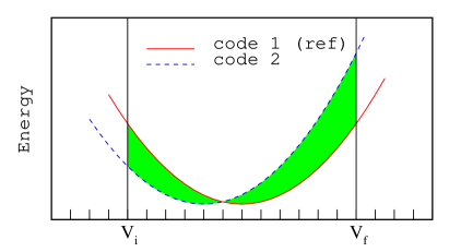
Figure 1: Schematic comparison of the EoS obtained by two codes. Code 1 is taken as a reference and the integration is centered around its minimum. The $\Delta$ factor is proportional to the mean square deviation of the two EoS. The energy difference between the two EoS, whose square enters in the definition of $\Delta$, is shown as the shaded area.

II.2 $\Delta$ Factor Calculations

In a recent work Lejaeghere et al. Lejaeghere2013 propose to assess the agreement of the DFT description provided by any two codes/methods by comparing their resulting equations of state. A quality factor $\Delta$, defined by the mean square deviation of the two EoS, is introduced as

$$\Delta=\sqrt{\frac{\int(\Delta E)^{2}(V)dV}{\Delta V}}$$ (2)

where $\Delta E$ is the difference between the energies given by the two codes/methods and $\Delta V$ is the volume integration interval taken as $\pm 6$ % around the equilibrium volume of the code taken as reference. In order to obtain the EoS they consider seven values around a reference volume $V_{ref}$ (0.94 $V_{ref}$ to 1.06 $V_{ref}$) and use the third order Birch-Murnaghan EoS (Eq. 1).

In Ref.Lejaeghere2013, , the comparison is performed among the EoS obtained by WIEN2k, GPAW and VASP for a set of 71 elements at their equilibrium structures. We extend their work to Elk and QE-PAW calculations, using the same procedure, $V_{ref}$ and structure files. Furthermore, we also consider a slightly modified definition for the quality factor, $\Delta^{\prime}$, that provides a well-defined distance between the codes/methods compared (see later Section III.3).

	valence	$r_{loc}$ (a.u.)		$r_{c}(a.u.)[\epsilon_{ref}$(Ry)$]$		$r_{\rm core}$ (a.u.)	$r_{sph}$ (Å)	$E_{cut}$ (Ry)
			s	p	d
Cs	$5s^{2}6s^{1}5p^{6}$	2.2	1.9	2.3  [4.0]	2.1  [0.3,4.3]	1.6	1.22	35-140
Be	$2s^{2}$	1.4 (d)	2.0  [6.5]	2.0  [6.3]	1.4  [0.3]	1.3	1.06	30-197
Sc	$3s^{2}4s^{2}3p^{6}3d^{1}$	2.0	1.3	1.5, 1.8  [3.3]	1.6  [0.3]	0.8	1.06	45-477
Ti	$3s^{2}4s^{2}3p^{6}4p^{0}3d^{2}$	2.1	1.7	1.8	1.7  [0.8]	0.7	1.11	50-740
Cr	$3s^{2}4s^{1}3p^{6}4p^{0}3d^{5}$	2.0	1.5	1.5, 1.7  [3.1]	1.7  [0.3]	0.7	1.06	50-240
Mn	$3s^{2}4s^{2}3p^{6}4p^{0}3d^{5}$	1.9	1.7, 1.6	1.9  [0.4]	1.6  [-0.3]	0.7	1.01	46-245
Zn	$3d^{10}4s^{2}4p^{0}$	1.7	2.2  [6.1]	2.3  [6.3]	1.8  [-0.6]	0.7	1.22	39-232
Y	$4s^{2}5s^{2}4p^{6}5p^{0}4d^{1}$	2.4	1.6	1.7	1.9  [0.3]	1.1	1.27	36-252
Nb	$4s^{2}5s^{1}4p^{6}5p^{0}4d^{4}$	1.5	1.4	1.7  [-0.5]	1.7  [0.2]	1.0	0.90	42-365
Mo	$4s^{2}5s^{1}4p^{6}5p^{0}4d^{5}$	1.4	1.3	1.7	1.7  [0.3]	1.0	0.90	50-450
Tc	$4s^{2}5s^{2}4p^{6}5p^{0}4d^{5}$	1.2	1.7, 1.1	1.7, 1.2	2.0  [0.3]	0.9	1.06	62-832
Ru	$4s^{2}5s^{2}4p^{6}5p^{0}4d^{6}$	1.4	1.7, 1.3	1.8, 1.3	1.8  [0.3]	0.9	0.95	62-800
Rh	$4s^{2}5s^{1}4p^{6}5p^{0}4d^{8}$	1.9	1.7, 1.3	1.7	1.9  [0.3]	0.9	1.01	55-439
Cd	$4d^{9.5}5s^{2}5p^{0.5}$	1.9	2.1   [2.3]	2.3  [8.0]	1.8  [4.3]	1.3	1.22	33-180
Hf	$5s^{2}6s^{2}5p^{6}6p^{0}5d^{2}$	2.5	1.6	1.6	1.7  [0.3]	1.2	1.32	43-175
Re	$5s^{2}6s^{2}5p^{6}6p^{0}5d^{5}$	2.1	1.4	1.5	1.55   [0.3]	1.1	1.11	54-216
Os	$6s^{2}6p^{0}5d^{6}$	2.4	2.4  [0.4]	2.9  [1.6]	2.1  [0.3]	1.31	1.53	31-124
Hg	$5d^{10}6s^{2}6p^{0}$	1.9	2.1  [2.3]	2.3  [8.0]	2.2  [4.3]	1.5	1.22	29-116
Ge	$3d^{10}4s^{2}4p^{2}$	2.2	2.1  [3.1]	2.2  [6.3]	1.85  [-0.4]	0.9	1.16	36-240
As	$4s^{2}4p^{3}$	2.0 (d)	1.8  [0.4]	2.0  [0.4]	2.0  [0.5]	1.6	1.06	20-103
Se	$4s^{2}4p^{4}$	1.9 (d)	1.8  [0.3]	2.0  [0.3]	1.9  [0.2]	1.4	1.06	21- 95
Br	$4s^{2}4p^{5}$	1.9 (d)	1.9  [-1.0]	1.8  [0.2]	1.9  [-0.5]	1.4	1.01	25-108
Sb	$5s^{2}5p^{3}$	2.2	2.2  [5.5]	2.3  [6.3]	2.5  [0.1,6.4]	1.62	1.32	33-132
Te	$4d^{10}5s^{2}5p^{4}$	2.1	2.0  [6.3]	2.4  [6.3]	1.7  [1.3]	0.9	1.27	43-211
I	$5s^{2}5p^{5}$	2.0 (d)	1.9  [-1.0]	1.8  [0.2]	2.0  [1.5]	1.41	1.06	24-109
Tl	$5d^{10}6s^{2}6p^{1}$	2.2	2.0  [5.5]	2.6  [6.5]	2.0  [-0.6]	1.5	1.38	35-150
Bi	$5d^{10}6s^{2}6p^{3}$	2.2	2.2  [5.4]	2.6  [6.5]	2.0  [-1.3]	1.4	1.38	43-172
Po	$5d^{10}6s^{2}6p^{4}$	1.8	2.0   [1.0]	2.2  [7.0]	1.6  [-1.5]	1.2	1.16	53-447
He	$1s^{2}$	1.1 (p)	1.2   [-0.1]	1.1  [0.1]			0.64	41-165
Ne	$2s^{2}2p^{6}$	1.1 (d)	1.5, 1.6  [6.3]	1.5  [-0.9]	1.1  [0.15]	0.4	0.85	37-257
Ar	$3s^{2}3p^{6}$	1.8 (d)	1.8  [0.2]	2.1  [0.2]	1.8  [0.2,0.45]	0.9	1.11	26-225
Kr	$4s^{2}4p^{6}$	1.8	1.8   [0.3]	1.7  [0.2]	2.0  [0.3, 0.7]	1.4	1.06	28-220

Table 1: Electronic configuration and the matching radii for the local potential ($r_{loc}$), partial waves ($r_{c}$), and core density ($r_{\rm core}$), and reference energies ($\epsilon_{ref}$) used in addition to the energy eigenvalues for the PAW datasets of the PSLibrary, tested in this paper and not reported elsewhere. The total radius of the PP (maximum of all matching radii) is given in $r_{sph}$. The estimates of the wavefunction and density cut-off energies required for these PPs are reported in the last column. Note that while the density cutoffs are rather transferable between different electronic environment calculations, wavefunction cutoffs can show a stronger dependence. For further, we refer to the PSlibrary filespslibrary .

II.3 All-electron FP-LAPW setup

II.3.1 FP-LAPW for CMST

For the CMST set, we start by calculating the EoS of fcc, bcc and sc phases varying the muffin-tin radii $R_{MT}$, with a reasonably high wavefunction expansion cut off in the interstitial region, defined by a maximum K-vector length $K_{max}$ (typically such that $R_{MT}K_{max}=9$) and a dense K-point grid of $12\times 12\times 12$ with a Gaussian smearing of $0.02$ Ry. We then choose the smallest muffin-tin radius that gives a smooth EoS curve. With very few exceptions, for a given element we were able to choose the same radius for all three phases, which resulted in a higher accuracy in energy differences, thanks to error cancellations. In the final calculations the expansion limit, $K_{max}$, for interstitial wavefunction and the analogous parameter, ${G}_{max}$, for the interstitial density and potential were chosen such that the total energy was converged within 1 meV/atom . The Brillouin zone sampling and Gaussian smearing width were further optimized to result in the same convergence in the total energy. (See Supplementary Material for a list of $R_{MT}$, $K_{max}$, ${G}_{max}$, k-grid and smearing width for each element.)

We use the default core-state occupations in Elk. For alkaline and alkaline-earth metals we use the default local orbitals provided with the exception of Ca, in which adding d-like local orbitals at an energy slightly above the Fermi energy results in a great improvement in the lattice constant prediction. For transition metals we add d-like and f-like local orbitals above the Fermi energy, following the suggestion given in Ref. Madsen2001, .

II.3.2 FP-LAPW for $\Delta$ factor

In order to calculate the $\Delta$ factor in an unbiased way the internal convergence parameters of Elk are set using default values whenever possible. In particular, default values for the muffin-tin radius, the core electron configuration and the local orbitals are used, except for a few elements (see Supplementary Material for details) where convergence and stability issues forced us to optimize $R_{MT}$.

Although the choice of using the default settings may bias results against Elk, we believe that it reflects a realistic situation, where end-users do not alter the default values unless a convergence or stability issue arises. The high accuracy limit for Elk has been assessed through CMST instead.

Basis-set convergence parameters $K_{max}$, ${G}_{max}$, and the Brillouin zone sampling and smearing width were optimized to ensure convergence of total energies well within 3 meV/atom. In order to distinguish metallic and insulating systems in an automatic way, an initial scanning of the electronic entropy with Gaussian smearing was used. For resulting metallic systems (except magnetic ones) the Methfessel-Paxtonmeth smearing method is employed. All calculations are performed with PBE exchange correlation functional (See Supplementary Material for a compilation of the converged parameters).

II.4 PAW setup

The QE-PAW datasets tested in this paper are distributed in the QEforge portalQEforge within the PSlibrary package, version 0.3.1pslibrary . The datasets for Li, Na, K, Rb, Mg, Ca, Sr, Ti, V, Co, Cu, Ga, Ge, Zr, Nb, Mo, Rh,Pd, Ag, In, Sn, Ba,Ta, W, Ir and Pb were previously reported in Ref. testrel, while those for H, B, C, N, O, F, Al, Si, P, S, Cl, Fe and Ni were described in Ref. Waleed, , while Pt and Au were discussed in Ref. PAWso, . As a reference we give in Table 1 the parameters for all the remaining 32 elements used in this work. Note that the PP details for Ti, Ge, Nb, Mo, Rh were also given in Ref. testrel, , but they have been improved by using the all-electron data calculated in this paper. For further details such as augmentation pseudization radii we refer to the PSlibrary filespslibrary .

II.4.1 PAW for CMST

For each element in the CMST, we perform total energy calculations (using LDA or PBE) in the fcc, bcc, and sc phases using the procedure discussed in Section II.1. We then use the EoS fit to determine an estimated equilibrium lattice constant, $a_{0}$. The kinetic energy cut-offs for both the wavefunctions and the charge density are determined by converging the total energy within 0.5 mRy at this $a_{0}$ estimate. We then chose 15 points in the $\pm 0.175$ $a.u.$ range around $a_{0}$, and calculate the final energy-volume curve. For the Brillouin zone (BZ) integration we use uniform shifted k-point grids of $n\times n\times n$, points where $n$ was varied in the range from 4 to 24. To increase the convergence rate we use Gaussian or Marzari-VanderbiltMV cold smearing. The convergence of the results with respect to the k-point sampling and smearing parameter are tested separately for each system to result in a convergence within 0.01 Å  in the lattice parameter. The equilibrium lattice parameter and bulk modulus are calculated from a fit of the energy-volume curves to the EoS of Eq. 1. The quality of the fit is found to be always very high, with a $\chi^{2}$ lower than $10^{-10}$ Ry², except in a few cases indicating that the initial estimate for $a_{0}$ has not been satisfactory. In these cases the procedure is repeated starting from the new estimate for $a_{0}$, obtaining finally an accurate fit.

II.4.2 PAW for $\Delta$ factor

For the $\Delta$ factor calculations, each element in the PSlibrary dataset is tested in its equilibrium structure as proposed in Ref. Lejaeghere2013, . All calculations are performed with the PBE exchange correlation functional.

In order to setup the computational parameters for the $\Delta$ factor calculations the planewave expansion cutoff, the BZ sampling and smearing-width are systematically varied to result in a 3 meV/atom absolute convergence for the total energy. As in the case of Elk FP-LAPW calculations an initial scanning of the electronic entropy with Gaussian smearing is used to identify metallic systems. For insulators BZ integrations are not critical and the total energy converges rapidly with respect to the number of k-points, while for metallic systems careful smearingMV /k-sampling is used to insure convergence (See Supplementary Material for a compilation of the converged parameters).

III Results

	$fcc$			$bcc$				$sc$
Element	$a_{0}$	$B_{0}$		$a_{0}$	$B_{0}$	$E_{tot}-E_{tot}^{fcc}$		$a_{0}$	$B_{0}$	$E_{tot}-E_{tot}^{fcc}$
Li	4.231 [ 1]	15.1 [-0.0]		3.361 [ 2]	15.2 [-0.0]	0.001 [ 1.1]		2.665 [ 2]	13.4 [ 0.2]	0.120 [ -1.2]
Na	5.111 [ -3]	9.1 [-0.1]		4.053 [ -2]	9.2 [ 0.0]	0.001 [ -0.7]		3.293 [ -3]	7.3 [-0.1]	0.124 [ -1.1]
K	6.358 [ 0]	4.5 [ 0.2]		5.040 [ -0]	4.5 [-0.1]	0.000 [ 0.2]		4.099 [ -2]	3.5 [-0.0]	0.109 [ 0.5]
Rb	6.779 [ -7]	3.6 [ 0.2]		5.370 [ -2]	3.6 [ 0.0]	0.001 [ -4.2]		4.388 [ -6]	2.8 [-0.0]	0.100 [ -0.2]
Cs	7.344 [-50]	2.4 [ 0.0]		5.806 [-35]	2.4 [ 0.1]	0.001 [ -3.9]		4.795 [-39]	1.9 [ 0.1]	0.097 [ 4.0]
Be	3.109 [ -8]	130.7 [ 3.8]		2.464 [ -8]	133.0 [ 1.5]	0.016 [ 3.3]		2.142 [ -5]	80.3 [ 0.2]	0.987 [ 15.4]
Mg	4.435 [ -5]	38.4 [ 0.8]		3.512 [ -9]	38.4 [ 0.8]	0.016 [ -1.7]		2.962 [ -5]	25.0 [ 0.5]	0.375 [ 7.2]
Ca	5.335 [ -7]	18.7 [ 0.5]		4.216 [-10]	19.0 [ 0.1]	0.010 [ 1.3]		3.362 [-13]	13.3 [-0.6]	0.379 [ 1.5]
Sr	5.794 [ -6]	14.4 [-0.0]		4.573 [ -9]	14.4 [-0.4]	-0.001 [ -0.2]		3.646 [ -8]	8.7 [-0.2]	0.382 [ -0.0]
Ba	6.032 [-30]	9.0 [ 0.2]		4.790 [-22]	10.1 [ 0.7]	-0.014 [ 5.2]		3.750 [ -9]	8.8 [ 0.5]	0.267 [ 9.1]
Sc	4.474 [ -1]	58.5 [ 0.0]		3.569 [ -2]	59.1 [ 0.2]	0.081 [ -1.5]		2.851 [ -2]	40.2 [-0.1]	0.701 [ -2.1]
Ti	4.006 [ -2]	121.9 [ 0.1]		3.169 [ -2]	118.3 [ 1.5]	0.040 [ -1.0]		2.553 [ 2]	92.8 [ 1.4]	0.739 [ 6.0]
V	3.731 [ 5]	199.7 [ 1.7]		2.932 [ -1]	206.7 [ 1.1]	-0.295 [ 8.9]		2.386 [ 2]	164.6 [-2.4]	0.617 [-52.0]
Cr	3.547 [ 4]	272.0 [ 2.4]		2.791 [ 4]	295.6 [ 2.8]	-0.414 [ 4.2]		2.280 [ 8]	218.2 [ 5.0]	0.595 [ 36.7]
Mn	3.433 [ 4]	327.5 [ 1.9]		2.726 [ 4]	327.3 [ 1.5]	0.096 [ 4.0]		2.231 [ 3]	253.2 [ 2.8]	0.891 [ -2.0]
Fe	3.378 [ 2]	339.6 [ 3.5]		2.700 [ 2]	321.5 [ 1.8]	0.351 [ 0.4]		2.213 [ 3]	252.1 [ 2.4]	1.001 [ 6.8]
Co	3.378 [ 2]	310.1 [ 7.6]		2.700 [ 2]	291.9 [ 7.2]	0.279 [ -4.1]		2.226 [ 3]	226.5 [ 5.8]	0.917 [ 21.1]
Ni	3.424 [ 1]	254.8 [ 6.0]		2.724 [ -1]	249.6 [ 6.6]	0.067 [ 0.1]		2.263 [ -1]	187.6 [ 4.7]	0.741 [ 16.1]
Cu	3.527 [ 4]	185.2 [ 0.9]		2.803 [ 3]	181.1 [ 2.5]	0.030 [ 8.3]		2.332 [ 3]	136.0 [ 2.0]	0.542 [ -9.6]
Zn	3.796 [-15]	95.4 [ 4.5]		3.022 [-10]	90.5 [ 4.1]	0.072 [ -5.3]		2.532 [ -9]	65.5 [ 4.9]	0.242 [ 22.5]
Y	4.905 [ -0]	45.2 [ 0.5]		3.918 [ -5]	44.3 [-0.6]	0.117 [ 5.5]		3.135 [ -1]	31.4 [-0.5]	0.759 [ -0.4]
Zr	4.422 [ 5]	101.5 [ 1.1]		3.486 [ 2]	96.8 [ 2.8]	0.019 [ -0.8]		2.835 [ 8]	80.4 [ 0.1]	0.810 [ 1.3]
Nb	4.138 [ 5]	177.7 [ 3.9]		3.250 [ 0]	194.4 [-7.7]	-0.330 [-33.8]		2.665 [ 2]	147.7 [ 0.8]	0.626 [ 24.0]
Mo	3.942 [ -2]	263.9 [ 5.6]		3.115 [ -1]	287.1 [ 7.6]	-0.438 [ 5.7]		2.556 [ 2]	217.7 [ 2.0]	0.744 [ 12.1]
Tc	3.816 [ -2]	333.5 [ 7.7]		3.036 [ -2]	329.5 [ 7.7]	0.201 [ -1.3]		2.491 [ -2]	254.2 [ 3.2]	1.010 [ 19.8]
Ru	3.755 [ -5]	341.3 [19.3]		3.006 [ -3]	309.5 [22.3]	0.557 [ 5.1]		2.468 [ -1]	258.2 [ 5.2]	1.102 [ 6.2]
Rh	3.758 [ 5]	312.9 [ 4.8]		3.010 [ 4]	285.8 [ 4.2]	0.412 [ -6.6]		2.482 [ 4]	227.2 [ 3.0]	0.886 [ 16.2]
Pd	3.846 [ 2]	223.6 [ 7.5]		3.060 [ 2]	216.7 [ 7.5]	0.063 [ 6.4]		2.542 [ 2]	163.3 [ 7.5]	0.606 [ 9.8]
Ag	4.011 [ 2]	136.1 [ 3.5]		3.191 [ -1]	132.9 [ 6.8]	0.035 [ -8.4]		2.653 [ 4]	103.0 [ 1.0]	0.411 [ 18.0]
Cd	4.321 [-14]	66.8 [ 2.8]		3.446 [ -9]	59.6 [ 4.4]	0.067 [ 0.9]		2.862 [ -6]	50.4 [ 2.0]	0.169 [ 2.2]

Table 2: LDA results for the equilibrium lattice constant $a_{0}$, bulk modulus $B_{0}$ and total energy difference with the fcc phase (expressed in Å, GPa and eV respectively) calculated with LAPW for the solids included in CMST. Deviation from LAPW of the PAW results are reported in square brackets (expressed in mÅ, GPa and meV respectively).

	$fcc$			$bcc$				$sc$
Element	$a_{0}$	$B_{0}$		$a_{0}$	$B_{0}$	$E_{tot}-E_{tot}^{fcc}$		$a_{0}$	$B_{0}$	$E_{tot}-E_{tot}^{fcc}$
Li	4.324 [ 1]	13.9 [-0.1]		3.433 [ 3]	14.0 [-0.0]	0.001 [ 1.2]		2.733 [-0]	12.5 [-0.3]	0.119 [ 2.2]
Na	5.298 [-5]	7.7 [-0.0]		4.201 [-3]	7.7 [-0.0]	-0.001 [ 1.7]		3.416 [-6]	6.1 [ 0.1]	0.120 [-1.4]
K	6.666 [-2]	3.5 [ 0.1]		5.284 [ 0]	3.6 [ 0.0]	-0.001 [ 1.7]		4.299 [-1]	2.8 [ 0.0]	0.104 [ 0.6]
Rb	7.160 [-12]	2.8 [ 0.1]		5.674 [-0]	2.8 [-0.1]	-0.001 [-3.1]		4.630 [-4]	2.1 [-0.0]	0.095 [ 2.5]
Cs	7.815 [-30]	1.9 [-0.0]		6.193 [-19]	1.9 [ 0.0]	0.001 [-2.7]		5.073 [-21]	1.5 [-0.0]	0.089 [ 3.5]
Be	3.157 [-5]	119.8 [ 0.3]		2.501 [-5]	124.1 [ 0.7]	0.017 [ 1.5]		2.174 [-4]	75.6 [-0.4]	0.923 [ 9.6]
Mg	4.519 [-1]	35.7 [-0.4]		3.577 [-4]	35.6 [-0.4]	0.018 [-3.6]		3.018 [ 1]	22.9 [-0.3]	0.369 [ 1.8]
Ca	5.533 [-16]	17.1 [ 0.3]		4.385 [-5]	16.2 [ 0.3]	0.016 [ 0.1]		3.521 [-11]	11.2 [-0.4]	0.391 [ 3.6]
Sr	6.029 [-5]	11.6 [-0.2]		4.765 [-8]	11.7 [-0.0]	0.006 [ 0.1]		3.852 [-9]	7.3 [-0.2]	0.383 [ 4.2]
Ba	6.399 [-37]	8.0 [ 0.1]		5.053 [-25]	8.5 [ 0.4]	-0.017 [-0.1]		3.981 [-14]	7.3 [ 0.9]	0.285 [ 6.3]
Sc	4.621 [-1]	51.0 [ 0.0]		3.678 [-1]	53.0 [ 0.4]	0.054 [ 1.1]		2.961 [ 5]	34.5 [ 0.2]	0.720 [-1.4]
Ti	4.114 [ -1]	107.0 [ 0.9]		3.256 [-1]	105.4 [ 0.6]	0.057 [-4.0]		2.638 [ 4]	76.4 [ 2.5]	0.778 [ 3.0]
V	3.820 [ 1]	174.0 [ 1.7]		2.997 [ 3]	181.7 [-0.8]	-0.244 [ 1.7]		2.447 [ 4]	137.4 [ 0.8]	0.596 [ 2.8]
Cr	3.624 [ 3]	236.0 [ 0.9]		2.851 [ 1]	256.2 [ 1.6]	-0.393 [ 2.5]		2.340 [ 3]	186.9 [ 0.2]	0.634 [-0.2]
Mn	3.506 [ 2]	278.3 [ 1.8]		2.785 [ 3]	276.6 [ 0.9]	0.081 [ 2.0]		2.285 [ 1]	210.1 [ 2.9]	0.866 [ 1.0]
Fe	3.452 [ 2]	283.8 [ 1.9]		2.761 [ 1]	266.3 [ 2.1]	0.312 [ 4.5]		2.269 [ 1]	206.2 [ 1.5]	0.948 [ 7.6]
Co	3.458 [ 3]	252.9 [ 4.8]		2.765 [ 2]	237.4 [ 4.5]	0.259 [-10.6]		2.284 [ 3]	182.2 [ 3.6]	0.856 [15.5]
Ni	3.516 [-1]	201.7 [ 3.4]		2.797 [-2]	197.8 [ 3.5]	0.055 [ 3.7]		2.327 [ 0]	146.3 [ 2.5]	0.661 [21.5]
Cu	3.635 [11]	139.8 [-1.1]		2.890 [ 8]	136.7 [-2.9]	0.033 [ 1.5]		2.410 [ 8]	101.5 [-1.4]	0.465 [-3.6]
Zn	3.940 [-14]	67.2 [ 1.5]		3.139 [-8]	61.4 [ 3.2]	0.062 [-0.6]		2.639 [-8]	45.7 [-2.3]	0.192 [62.0]
Y	5.067 [-3]	39.3 [ 0.1]		4.043 [-0]	38.9 [-0.1]	0.099 [-2.5]		3.264 [ 4]	25.9 [-0.0]	0.772 [-0.1]
Zr	4.531 [ 2]	89.7 [ 0.8]		3.577 [ 2]	86.7 [ 0.6]	0.054 [-10.6]		2.916 [ 3]	68.6 [ 1.9]	0.834 [ 2.5]
Nb	4.223 [-4]	160.2 [ 4.1]		3.314 [-3]	166.3 [ 7.5]	-0.321 [-2.7]		2.722 [-2]	127.7 [ 3.2]	0.649 [ 7.9]
Mo	4.007 [-4]	234.1 [ 5.3]		3.165 [-3]	254.6 [ 5.4]	-0.424 [-3.7]		2.609 [-8]	184.9 [14.1]	0.723 [-2.0]
Tc	3.876 [-3]	291.7 [ 8.1]		3.084 [-3]	287.7 [ 5.8]	0.182 [-0.4]		2.535 [-2]	217.5 [ 4.1]	0.965 [12.2]
Ru	3.814 [-2]	302.5 [ 3.5]		3.055 [-0]	276.8 [ 5.2]	0.512 [ 3.2]		2.513 [ 0]	217.5 [ 3.0]	1.015 [ 5.6]
Rh	3.833 [13]	253.7 [-0.1]		3.073 [10]	230.1 [ 3.5]	0.362 [-11.8]		2.538 [10]	180.4 [ 2.2]	0.789 [-10.1]
Pd	3.946 [ 4]	166.5 [ 1.2]		3.141 [ 3]	162.0 [ 1.0]	0.042 [-2.0]		2.617 [ 3]	119.4 [ 1.8]	0.499 [-1.6]
Ag	4.155 [ 1]	88.6 [ 6.4]		3.306 [-2]	87.8 [ 3.8]	0.025 [-4.4]		2.757 [-2]	65.0 [ 3.3]	0.319 [27.0]
Cd	4.519 [-17]	39.8 [ 2.4]		3.614 [-13]	34.3 [ 2.9]	0.048 [ 1.9]		3.007 [-11]	28.2 [ 2.3]	0.108 [10.9]

Table 3: PBE results for the equilibrium lattice constant $a_{0}$, bulk modulus $B_{0}$ and total energy difference with the fcc phase (expressed in Å, GPa and eV respectively) calculated with LAPW for the solids included in CMST. Deviation from LAPW of the PAW results are reported in square brackets (expressed in mÅ, GPa and meV respectively).

III.1 Comparison of LAPW data with literature results

Motivated by the technical nature of the calculations, before providing our findings, we first verify our LAPW calculations with existing results in the literature, given that some of the crystals included in the CMST were present in published work Haas2009 ; Haas2009err ; Tran2007 . For example Ref. Haas2009, shares with our test 16 cases out of 90. The relative lattice constant difference between these is less than 0.16%; exceptions are Fe $bcc$ which shows a large discrepancy (around 2% both for LDA and PBE) and Ba $bcc$ (-0.76% in LDA). Ref. Tran2007, reports the bulk modulus of the same systems: the lattice constants can be seen to be identical to Ref. Haas2009, (apart for those specified in the errataHaas2009err ). The relative difference in bulk moduli between Ref. Tran2007, and our present results is less than 3.2%, the only exception being Fe $bcc$. These differences between two independent FP-LAPW calculations give an estimate of a lower bound for the accuracy to be targeted in a PAW and FP-LAPW comparison.

Unfortunately other all-electron data available in literature are limited to a small number of crystalline systems and/or are calculated with different techniques. As an example, Ref. Ropo2008, reports exact muffin-tin orbitals (EMTO) results. EMTO is a method of the Korringa-Kohn-Rostoker type, credited to be as accurate as full-potential methods. Ropo2008 ; Asato1999 Ref. Ropo2008, and this study have 18 systems in common. The relative lattice constant difference is less than 0.5%; exceptions being Fe, Ba and Cs $bcc$ in LDA, and Ni $fcc$ in PBE. The relative difference in bulk moduli is less than 5% in approximately half of the cases and larger in the remaining cases, up to 28% for Fe $bcc$ in PBE. These relative differences are greater than the ones found with respect to the FP-LAPW calculations,Haas2009 ; Tran2007 and are of the same order as the difference between other LAPW resultsHaas2009 ; Tran2007 and the EMTO results. Ropo2008

Another example is Ref. Mattsson2008, , which reports calculations performed with the full-potential linear muffin-tin orbital method (LMTO). Only 6 systems are common and the results are quite close both in terms of $a_{0}$ and $B_{0}$, differences being at most 0.3 % in the lattice parameter and 2 % in the bulk modulus.

The Elk FP-LAPW CMST database expands and fills the gaps in all-electron data available in the literature providing an extensive set of systems, generated by a uniform procedure in terms of computational method used and convergence parameters, that includes several simple structures for each element and reports both structural properties and energy differences. While the choice of cubic structures for CMST is at variance with present tests in the literature that mostly focus on the experimental stable phases, it allows an extensive comparison of the energetics of $fcc$, $bcc$ and $sc$ phases which we believe are of interest for rapidly assessing the performance of a computational methodology in the most homogeneous way.

III.2 CMST comparison between PAW and FP-LAPW data

We report in Table 2 and 3 the all-electron FP-LAPW values for the equilibrium lattice constants ($a_{0}$), the bulk moduli ($B_{0}$) and the energy differences between the three phases obtained using LDA and PBE respectively. The energies of the bcc and sc structures are referenced to fcc case. A negative value of the difference indicates that the structure is more stable than the fcc one. Results for the PAW calculations are also reported in square brackets as differences with respect to the LAPW values. In Figs. 2 and 3 the PAW-LAPW differences in $a_{0}$ and $B_{0}$ are plotted as a percentage of the all-electron LAPW value. In Fig. 4 PAW and LAPW energy differences between phases are reported as well as the difference between PAW and LAPW results.

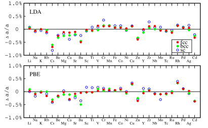
Figure 2: Percentage differences between LAPW and PAW lattice constants for the solids included in CMST, in all three crystalline phases considered, calculated using LDA (top ) and PBE (bottom) functionals.

We start by discussing the differences in lattice constant between PAW and LAPW calculations (Fig. 2). For almost all elements and structures the PAW-LAPW discrepancy on the lattice constant is well below 0.4%. There are some notable exceptions: Ba (fcc and bcc), and Cs (fcc, bcc and sc), in LDA; Ba (fcc and bcc), Cs (sc) and Rh (sc) in PBE, with the worst cases being Cs sc (-0.8%) in LDA and Ba fcc (-0.57%) in PBE. Most elements/structures show discrepancies smaller than 0.2%: 78 and 75 out of 90 in LDA and PBE respectively. Overall, the mean PAW-LAPW difference is very small both in LDA and PBE ( -0.065% and -0.055% respectively). The discrepancies between PAW and FP-LAPW in the fcc, bcc, and sc lattice constants are not independent from each other as can be seen from the linear correlation coefficients in Table 4. This high degree of correlation is quite important as it suggests that the pseudopotentials employed have excellent transferability among the electronic environments tested.

	$fcc$		$bcc$		$sc$
$fcc$	1		0.92		0.86
$bcc$	0.94		1		0.89
$sc$	0.90		0.88		1

Table 4: Correlation matrix between PAW and FP-LAPW differences for the equilibrium lattice constant $a_{0}$ in the fcc, bcc, and sc structures. The upper half of the matrix shows LDA results while the lower half of the matrix shows PBE results. A correlation matrix element close to 1 indicates a strong correlation, highlighting that the performance of the pseudopotentials used in this work is similar in the different electronic environments considered.

Overall, from the data collected it appears that the comparison between PAW and FP-LAPW is slightly closer for PBE than for LDA. Also, we find that for some elements the treatment of the semicore electrons has a significant effect, in particular for Cs and Ba the inclusion of the $4d$ electrons in the core would result in smaller lattice parameters by as much as 0.03 Å in the LAPW calculations. Due to this effect here we report Elk results with $4d$ electrons in valence for the case of Ba and Cs. However, the impact of semicore states appears less important in the PAW calculations; therefore the results reported use PAW datasets with $4d$ electrons in the core.

Similar PAW calculations have been reported in Ref. GBRV, ; however, in that study a fixed cut-off of $40$ Ry has been used for all elements to optimize sets for high-throughput calculations. Although for many elements there is agreement between our data and those of Ref. GBRV, , in some cases, such as Li and Cu, the relatively large deviation reported in that work is not confirmed by our calculations. We attribute this difference to the use of insufficient number of planewaves in Ref. GBRV, . On the contrary, in the case of Cd both our calculations and the ones in Ref. GBRV, consistently show a relatively large deviation from all-electron results.

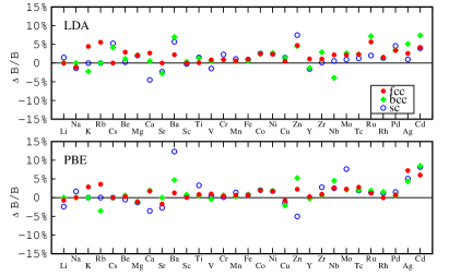
Figure 3: Percentage differences between LAPW and PAW bulk moduli for the solids included in CMST, in all three crystalline phases considered, calculated using LDA (top ) and PBE (bottom) functionals.

The PAW - FP-LAPW deviations for the bulk moduli are reported in Fig. 3. For most of the elements and structures studied, the PAW - FP-LAPW difference is less than 6%. The exceptions are K (fcc), Rb (fcc), Cs (bcc), Ba (bcc and sc), Zn (sc), Ru (fcc and bcc), Ag (bcc), and Cd (bcc) in LDA; Ba (sc), Zn (bcc and sc), Mo (sc), Ag (fcc and sc), and Cd (fcc, bcc and sc) in PBE. The average deviation between PAW and LAPW bulk moduli is 1.7% for LDA and 1.3% for PBE, with a general trend of PAW overestimating FP-LAPW $B_{0}$.

Our calculations reveal that, contrary to common expectation, the percentile deviation on $B_{0}$ is not tightly correlated with the corresponding deviation on $a_{0}$: the linear correlation coefficient between these two data sets can be as low as -0.26 for LDA and -0.31 for PBE.

We report the PAW - FP-LAPW deviation for the $bcc$-$fcc$ and $sc$-$fcc$ energy differences in Fig. 4 While we require an accuracy of the order of a few mRy in the transferability tests of the PPs, this error is usually an upper limit and for many elements the energy differences between different phases agree with the all-electron results within a few meV. A deviation larger than 13 meV ($\approx$1 mRy) in the $bcc$-$fcc$ energy difference is found only for Nb in LDA. The arithmetic average of the PAW - FP-LAPW deviations are as small as 2 meV and -1 meV in LDA and PBE, with a standard deviation of 14 meV and 4 meV respectively. The PAW - FP-LAPW discrepancies in the $sc$-$fcc$ energy difference are somewhat larger than the ones for $bcc$-$fcc$ energy difference, consistent with the larger average value of these differences. Choosing a threshold of 26 meV ($\approx$ 2 mRy) one can identify V and Cr as the elements needing further attention in LDA and Zn and Ag in PBE. The arithmetic average of the PAW - FP-LAPW deviations are 9 meV and 7 meV for LDA and PBE, with 19 meV and 6 meV standard deviation respectively. The $sc$-$fcc$ PAW - FP-LAPW deviations appear to be positive biased, while $bcc$-$fcc$ are centered around zero. Overall, in the case of the widely used PBE functional, an excellent agreement between our PAW datasets and LAPW results can be seen.

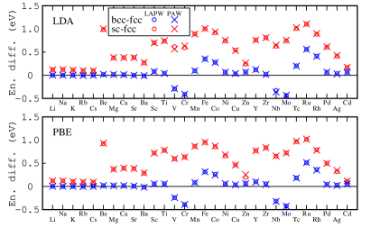
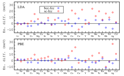
Figure 4: (a) CMST absolute energy difference (eV) (with respect to fcc) for the bcc and sc phases, for both FP-LAPW and PAW, using LDA (top) and PBE (bottom). (b)Absolute differences (meV) between FP-LAPW and PAW estimates for the energy differences between the bcc-fcc and sc-bcc pairs, using LDA (top) and PBE (bottom).

Results for alkaline-metal and alkaline-earth elements deserve a word of caution. Our FP-LAPW calculations have been converged within 1 meV/atom and the transferability of the QE-PAW datasets was verified to be of a few mRy in a number of atomic configurations. As the energy difference between fcc and bcc structures in alkaline and alkaline-earth metals are of the order of 1 meV and 1 mRy respectively, some difficulty in accurately reproducing these within the present study can be expected. Nevertheless, general trends seem in agreement with literature. As an example, in Li, K, and Rb the $fcc$ structure is known to be more stable than the $bcc$ when using LDA. Sliwko1996 ; Nobel1992 We confirm these results both for LAPW and PAW, except for Rb within PAW which is stable in the $bcc$ structure. For alkaline-earth elements LAPW and PAW calculations show identical outcomes, identifying correctly the experimental equilibrium phase for Ca ($fcc$), and Ba ($bcc$). The equilibrium phase in Be and Mg is the hexagonal-close packed ($hcp$) structure not included in our test set; still, we notice that the close-packed $fcc$ phase is favored with respect to $bcc$ in these two elements, as could be expected. The bcc-fcc energy difference in Sr is very small, just a few meV, and only PBE (both within PAW and LAPW) captures the correct ($fcc$) ground state phase.

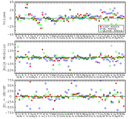
Figure 5: Comparison of EoS parameters between QE-PAW dataset, VASP PAW, FP-LAPW results from Elk and WIEN2k. The zero reference is chosen as WIEN2k for all elements considered in the $\Delta$ factor calculations. All calculations are performed using PBE exchange-correlation functional; VASP and WIEN2k values taken from Ref. Lejaeghere2013, .

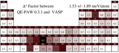
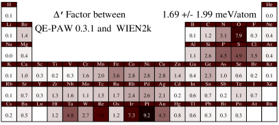
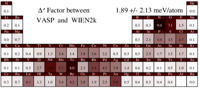
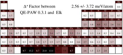
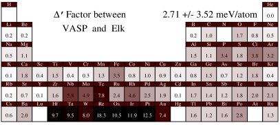
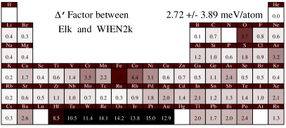
Figure 6: $\Delta^{\prime}$ factor comparison between QE-PAW, VASP PAW and FP-LAPW results from Elk and WIEN2k. $\Delta^{\prime}$ is a symmetric measure that qualifies as a distance between the codes/methods considered as it obeys the triangular inequality criterion. For each pair we provide the average distance as well as individual distances per element. Color codes are linear with respect to distances. All calculations are performed with the PBE exchange correlation functional. VASP and WIEN2k values are taken from Ref. Lejaeghere2013,

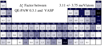
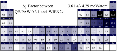
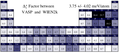
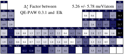
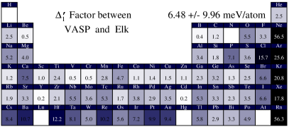
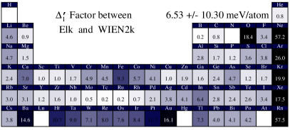
Figure 7: $\Delta_{1}^{\prime}$ factor comparison between QE-PAW, VASP PAW and FP-LAPW results from Elk and WIEN2k. $\Delta_{1}^{\prime}$ is a symmetric and positive-definite measure and does not qualify as a distance. However, this measure removes the bias of the original $\Delta$ factor with respect to stiffness and therefore yields a criteria to assess differences between codes/methods that is more homogeneous over all periodic table. For each pair we provide the average $\Delta_{1}^{\prime}$ and the standard deviation, as well as the individual distance for each element. Color codes are linear with respect to $\Delta_{1}^{\prime}$ factor. All calculations are performed with the PBE exchange correlation functional. VASP and WIEN2k values are taken from Ref. Lejaeghere2013,

III.3 $\Delta$ Factor across the periodic table

In this section we present the results of the calculation of the structural properties of a large majority of the elements in the periodic table (68) in their experimental equilibrium phase, (or occasionally a simpler, closely related one), obtained following the procedure described in Ref. Lejaeghere2013, .

Results obtained by four codes are compared: i) Elk LAPW calculations performed following the protocol described in section II.3 ii) QE-PAW calculations as described in section II.4 iii) VASP and iv) WIEN2k results from the literature. The data for VASP and WIEN2k have been determined in Ref. Lejaeghere2013, and made available online at the CMM website CMM-website , and the most recent values available at the website are used here.recent In our QE-PAW calculations results for all elements discussed in Ref. Lejaeghere2013, are presented, with the exception of Lu, Rn and Xe whose datasets are still under development. Elk calculations for H, N, Lu and Hg are also excluded due to convergence problems.

In Fig. 5 we display the relative deviation from the WIEN2k results of the structural parameters $V_{0}$, $B_{0}$ and $B_{0}^{\prime}$, obtained fitting Eq. 1 to the Elk and QE-PAW calculations. For completeness, the VASP results are also included. All numerical values of all these parameters are given in full in the Supplementary Material.

We can see that values predicted by different computational methods show a different spread depending on the property considered. The equilibrium volume has a typical variation of 1-2%, although larger deviations are occasionally present, while the bulk modulus has a larger spread of 5-10%, and its pressure derivative an even larger one.

In order to quantify in a single figure the agreement between the results of different codes Lejaeghere and coworkersLejaeghere2013 introduced a quality factor $\Delta$, measuring the discrepancy between the corresponding two EoS (see section II.2 above). In the original definition of $\Delta$ the volume integration is defined as a fixed $\pm$6% interval around the equilibrium volume obtained for one of the two methods (WIEN2k in their case) that is taken as a reference. This approach cannot be completely satisfactory because it results in an asymmetric comparison, since it depends on the choice of a reference data set among the two elements of each comparison. Instead, having access to a measure of the distance between the results of two codes/methods rather than taking one of the two as an absolute reference could provide further insight in the comparison as the number of codes/methods to compare increases.

We tried to correct for this by defining a symmetric quality factor $\Delta_{sym}$ where the volume integration in Eq. 2 is performed in the $\pm$6% interval around the average equilibrium volumes predicted by the two methods being compared. We note that $\Delta_{sym}$, although being a symmetric and positive definite function, fails to satisfy the triangular inequality for the distances between any three codes/methods, also explicitly checked on the available data.

We therefore introduce a slightly modified quality factor $\Delta^{\prime}$ defined so that the volume integral is performed in the $\pm$6% interval around the reference volume $V_{ref}$ used to generate the 7 points in the energy-volume curve which are used to determine the EoS. The resulting $\Delta^{\prime}$ defines a proper distance between pairs of codes/methods for each element. Very satisfactorily, the computed $\Delta^{\prime}$ values differ only slightly from the original $\Delta$ values, while being a well defined distance between codes and methods.

In Fig. 6 we display the results of the $\Delta^{\prime}$ factors across the periodic table comparing Elk, VASP, WIEN2k, and QE-PAW. On average the four codes/methods agree very well with each other. The two that are closest are QE-PAW and VASP (1.53 meV/atom), WIEN2k is only marginally more distant (1.69-1.89 meV/atom) and Elk is slightly farther away (2.56-2.72 meV/atom) due to the contributions of the $5d$ transition metal elements. This discrepancy between two all-electron calculations highlights the importance of standardized verification and validation tests, and indicates that optimization of computational parameters plays an important role in the outcome of the FP-LAPW calculations. Other elements for which noticeable discrepancies between methods are visible are certain transition metals and the second half of the elements of the first row, revealing once more the elements which require careful treatment within DFT, where small changes in implementation can have a significant impact in the outcome. Besides these cases, all methods give consistently very close results.

It has been pointed out in Ref. JTH, that the value of $\Delta$ factor strongly depends on the stiffness of the material and on its volume per atom. The larger the bulk modulus or the atomic volume of a given element is, the larger the $\Delta$ value associated to a given deviation of the structural parameters becomes.

A “renormalized” $\Delta_{1}$ factor has been proposedJTH ,

$$\Delta_{1}=\frac{V_{ref}B_{ref}}{V_{0}B_{0}}\Delta,$$ (3)

where the original value of $\Delta$ is scaled by the ratio of the equilibrium volume and the bulk modulus with respect to some reference values, taken to be $V_{ref}=30$ Å, $B_{ref}=100$ GPa, that roughly correspond to their average values over the elements.

The resulting $\Delta_{1}$ factor gives a more homogeneous measure of the quality of the agreement between codes across the periodic table.

We define a modified $\Delta_{1}^{\prime}$ rescaling the previously defined $\Delta^{\prime}$ factor via Eq.3 and taking for each element $V_{0}$ as the central value of the volume integration interval and $B_{0}$ as the average of the bulk moduli computed for the two codes/methods to be compared. $\Delta_{1}^{\prime}$ is no more a well-defined distance; however, it is imperative to analyze the results with this quality factor to understand better the effects of stiffness and volume per atom on EoS comparisons.

In Fig. 7 we display the result for the $\Delta_{1}^{\prime}$ factor calculations across the periodic table for the four codes/methods. On average $\Delta_{1}^{\prime}$ values are doubled with respect to $\Delta^{\prime}$.

		$\Delta$	$\Delta^{\prime}$	$\Delta_{1}$	$\Delta_{1}^{\prime}$
WIEN2k	QE	1.70 (1.70)	1.69	4.18  (3.46)	3.61
WIEN2k	VASP	1.92 (1.89)	1.89	3.79  (3.78)	3.75
WIEN2k	Elk	2.73 (2.71)	2.72	13.27  (5.55)	6.53
Elk	QE	2.58 (2.64)	2.56	5.78  (6.96)	5.26
Elk	VASP	2.72 (2.71)	2.71	5.33 (11.72)	6.48
QE	VASP	1.56 (1.53)	1.53	2.97  (3.79)	3.11

Table 5: PBE results for various $\Delta$ factor definitions in meV. For $\Delta$ and $\Delta_{1}$ factors, which are not symmetric, in parenthesis we give the reverse comparison result where the second method is chosen as the reference instead.

Again, the two codes/methods that result to be closest are QE-PAW and VASP (3.11 meV/atom). WIEN2k is only marginally more distant from each of them, (3.61-3.75 meV/atom) while Elk is farther away (5.25-6.53 meV/atom). Examining the data one can confirm that the second half of the elements of the first row as well as elements in the transition metal series remain problematic, although $5d$ elements appear less so here than when considering the $\Delta^{\prime}$ factor. Another class of potentially challenging elements are the noble gases, for which the values of the original $\Delta^{\prime}$ factor were systematically very small due to the very low value of their bulk moduli. We have thus re-examined further the EoS for the noble gases. It is found that the energy differences in EoS are within the convergence limit of our calculations for Ar, Kr, Xe in Elk and Ne in QE-PAW. These findings reveal that the bias of the original $\Delta^{\prime}$ factor with respect bulk moduli can be overcome with the use of $\Delta_{1}^{\prime}$.

In Table 5 we provide a final summary of our results using all variations of $\Delta$ factors that have been proposed so far. Our results show that for all the variations in the $\Delta^{\prime}$ factor, all the compared codes/methods agree well within 15 meV. We also see that rather than an average over the periodic table, an element-by-element analysis of the quality factor, together with the EoS when necessary, highlights the elements that could benefit from improvement in each computational approach. Following these indications our efforts towards more standardized pseudopotentials continue (see the experimental pseudization recipes in PSLibrary v1.0.0 dalcorso100 ).

IV Conclusions

In this study we have introduced a Crystalline Monoatomic Solid Test protocol comprising the calculation of the structural properties and relative energy differences of the three crystalline non-magnetic cubic phases ($sc$, $fcc$, and $bcc$) of any given element. While most results in the literature focus on experimentally stable phases, these results provide an extensive comparison of the energetics of simple but realistic structural phases that explore several coordination numbers, thus providing key information to assess and compare the performance of different computational methodologies.

We have collected a database of carefully performed all-electron FP-LAPW results, obtained by the Elk open-source code, and plane-wave PAW results, obtained by the Quantum ESPRESSO distribution including QE-PAW datasets from the PSlibrary, for a large fraction of the periodic table, including the alkaline-metals, the alkaline-earth and the $3d$ and $4d$ transition-metal elements (a total of 30 elements).

The CMST protocol reveals that for the majority of the systems tested QE-PAW and Elk LAPW show excellent agreement in equilibrium lattice parameter within 0.4%, in bulk modulus within 6% and in energy differences within 1mRy, both in PBE and LDA, with the overall agreement slightly better for PBE. While performing the CMST, in the case of alkaline and alkaline-earth metals we have observed convergence and stability issues which point to a need for further studies that quantify the importance of the treatment of core electrons as well as the need of robust implementations.

In the $\Delta$ factor tests, we have further extended the comparison between LAPW and PAW for 68 elements in the periodic table, following the protocol recently proposed by Ref.Lejaeghere2013, et al., based on a standardized study of the equation of state of the elements in their experimental equilibrium phase. We have provided a second all-electron reference for this test set using the default values of Elk (unless a stability or converge issue has been encountered), to represent a realistic scenario of the end-uses of all-electron methods, and given that the agreement between QE-PAW and Elk has already been demonstrated by the CMST in the case of careful tuning. We have also extended the definition of the quality factor to $\Delta^{\prime}$, a measure from which a proper distance satisfying the triangular inequality between codes/methods can be derived, allowing reference-independent comparisons.

For all flavors of the quality factor $\Delta$, and for the majority of the periodic table, we have found good agreement between the QE-PAW data, the Elk data, and the WIEN2k and VASP data from the literature. This agreement highlights the reliability of the current state-of-the-art electronic structure codes/methods for a wide range of elements in the periodic table. The differences observed for the remaining elements call attention to the urgent need of establishing reference data sets and standards for verification and validation among computational approaches, both at the highest accuracy limit and for optimal, practical applications by end-users.

Finally, the extensive tests we provide make the PSLibrary v0.3.1 a reliable default choice to be used within planewave pseudopotential implementations, that is openly available, updated and supported epfl_pseudo_repository .

- (1) G. Onida, L. Reining and A. Rubio, Rev. Mod. Phys. 74, 601 (2002).
- (2) R. Martonak, D. Donadio, A. R. Oganov and M. Parrinello, Nature Materials 5 623 (2006).
- (3) S. Curtarolo, G. L. W. Hart, M. Buongiorno Nardelli, N. Mingo, S. Sanvito, and O. Levy, Nature Materials 12 191 (2013).
- (4) A. Jain, S.P. Ong, G. Hautier, W. Chen, W.D. Richards, S. Dacek, S. Cholia, D. Gunter, D. Skinner, G. Ceder and K.A. Persson, Applied Physics Letters Materials 1 011002 (2013).
- (5) N. Marzari, MRS Bulletin 31 681 (2006).
- (6) D. R. Hamann, M. Schlüter, and C. Chiang, Phys. Rev. Lett. 43, 1494 (1979).
- (7) D. Vanderbilt, Phys. Rev. B 41, 7892 (1990).
- (8) P.E. Blöchl, Phys. Rev. B 50, 17953 (1994).
- (9) G. Kresse, D. Joubert, Phys. Rev. B 59, 1758 (1999).
- (10) L.A. Curtiss, K. Raghavachari, G.W. Trucks, and J.A. Pople, J. Chem. Phys. 94, 7221 (1991).
- (11) J. C. Grossman, J. Chem. Phys. 117, 1434 (2002).
- (12) N. Nemec, M.D. Towler, and R.J. Needs, J. Chem. Phys. 132, 034111 (2010).
- (13) J. Paier, R. Hirschl, M. Marsman, and G. Kresse, J. Chem. Phys. 122 234102 (2005).
- (14) P. Blaha,K. Schwarz, G. K. H. Madsen, D. Kvasnicka, J. Luitz: WIEN2k, 1999. “An augmented plane wave + local orbitals program for calculating crystal properties, Karlheinz Schwarz”. Austria: Techn. Universität Wien. ISBN:3-9501031 http://www.wien2k.at
- (15) J. Enkovaara, C. Rostgaard, J. J. Mortensen, J. Chen, M. Dulak, L. Ferrighi, J. Gavnholt, C. Glinsvad, V. Haikola, H. A. Hansen, et al. J. Phys.: Condens. Matter 22, 253202 (2010) https://wiki.fysik.dtu.dk/gpaw/
- (16) G. Kresse and J. Hafner. Phys. Rev. B 49, 14251 (1994). G. Kresse and J. Furthmüller. Comput. Mat. Sci. 6, 15 (1996). G. Kresse and J. Furthmüller. Phys. Rev. B 54, 11169 (1996). https://www.vasp.at
- (17) K. Lejaeghere, V. Van Speybroeck, G. Van Oost, and S. Cottenier, Critical Reviews in Solid State and Materials Sciences 39, 1 (2014); arXiv:1204.2733.
- (18) K.F. Garrity, J.W. Bennet, K.M. Rabe, and D. Vanderbilt, Computational Materials Science 81, 446-452 (2014); arXiv:1305.5973.
- (19) http://elk.sourceforge.net
- (20) http://www.qe-forge.org/gf/project/pslibrary. Note that among the tested elements the only differences between versions 0.3.0 and 0.3.1 occur for Ti, Cd, Ge, Te, Mn, Re, Po, Sb and Xe.
- (21) P. Giannozzi, S. Baroni, N. Bonini, M. Calandra, R. Car, C. Cavazzoni, D. Ceresoli, G. L. Chiarotti, M. Cococcioni, I. Dabo, A. Dal Corso, S. Fabris, G. Fratesi, S. de Gironcoli, R. Gebauer, U. Gerstmann, C. Gougoussis, A. Kokalj, M. Lazzeri, L. Martin-Samos, N. Marzari, F. Mauri, R. Mazzarello, S. Paolini, A. Pasquarello, L. Paulatto, C. Sbraccia, S. Scandolo, G. Sclauzero, A. P. Seitsonen, A. Smogunov, P. Umari, R. M. Wentzcovitch, J. Phys.: Cond. Matter, 21, 395502 (2009). http://www.quantum-espresso.org/
- (22) J.P. Perdew K. Burke and M. Ernzerhof, Phys. Rev. Lett. 77, 3865 (1996).
- (23) J.P. Perdew and A. Zunger, Phys. Rev. B 23, 5048 (1981).
- (24) Georg K.H. Madsen, Peter Blaha, Karlheinz Schwarz, Elisabeth Sjöstedt, and Lars Nordström Phys. Rev. B 64, 195134 (2001).
- (25) M. Methfessel, and T. Paxtox, Phys. Rev. B 40, 3616 (1989).
- (26) N. Marzari, D. Vanderbilt, A. De Vita, and M.C. Payne, Phys. Rev. Lett. 82, 3296 (1999).
- (27) http://www.qe-forge.org/
- (28) A. Dal Corso, Phys. Rev. B 86, 085135 (2012).
- (29) A. A. Adllan and A. Dal Corso, J. Phys.: Condens. Matter 23, 425501 (2011).
- (30) A. Dal Corso, Phys. Rev. B 82, 075116 (2010).
- (31) P. Haas, F. Tran, and P. Blaha, Phys. Rev. B 79, 085104 (2009).
- (32) F. Tran, R. Laskowski, P. Blaha, and K. Schwarz, Phys. Rev. B 75, 115131 (2007).
- (33) P. Haas, F. Tran, and P. Blaha, Phys. Rev. B 79, 209902(E) (2009).
- (34) M. Ropo, K. Kokko, and L. Vitos, Phys. Rev. B 77, 195445 (2008).
- (35) M. Asato, A. Settels, T. Hoshino, T. Asada, S. Blügel, R. Zeller, and P. H. Dederichs, Phys. Rev. B 60, 5202 (1999).
- (36) A. E. Mattsson, R. Armiento, J. Paier, G. Kresse, J. M. Wills, and T. R. Mattsson, J. Chem. Phys. 128, 084714 (2008).
- (37) V.L. Sliwko, P. Mohn, K. Schwarz and P. Blaha, J. Phys.: Condens. Matter 8 799.
- (38) J.A. Nobel and S. B. Trickey, P. Blaha and K. Schwarz, Phys. Rev. B 45, 5012.
- (39) http://molmod.ugent.be/DeltaCodesDFT
- (40) The Delta calculation package (version 2.0) distributed on the CMM web-siteCMM-website and the data therein have been used for the present calculations.
- (41) F. Jollet, M. Torrent, and N. Holzwarth. Comp. Phys. Commun. 185, 1246 (2014). ”Generation of Projector Augmented-Wave atomic data: a 71 elements validated table in the XML format”, arXiv:1309.7274v2
- (42) A. Dal Corso, to be published.
- (43) Pseudopotential repository at http://theossrv1.epfl.ch/Main/Pseudopotentials