Numerical study of the long wavelength limit of the Toda lattice

Abstract

We present the first detailed numerical study of the Toda equations in $2+1$ dimensions in the limit of long wavelengths, both for the hyperbolic and elliptic case. We first study the formal dispersionless limit of the Toda equations and solve initial value problems for the resulting system up to the point of gradient catastrophe. It is shown that the break-up of the solution in the hyperbolic case is similar to the shock formation in the Hopf equation, a $1+1$ dimensional singularity. In the elliptic case, it is found that the break-up is given by a cusp as for the semiclassical system of the focusing nonlinear Schrödinger equation in $1+1$ dimensions.

The full Toda system is then studied for finite small values of the dispersion parameter $\epsilon$ in the vicinity of the shocks of the dispersionless Toda equations. We determine the scaling in $\epsilon$ of the difference between the Toda solution for small $\epsilon$ and the singular solution of the dispersionless Toda system. In the hyperbolic case, the same scaling proportional to $\epsilon^{2/7}$ is found as in the small dispersion limit of the Korteweg-de Vries and the defocusing nonlinear Schrödinger equations. In the elliptic case, we obtain the same scaling proportional to $\epsilon^{2/5}$ as in the semiclassical limit for the focusing nonlinear Schrödinger equation. We also study the formation of dispersive shocks for times much larger than the break-up time in the hyperbolic case. In the elliptic case, an $L_{\infty}$ blow-up is observed instead of a dispersive shock for finite times greater than the break-up time. The $\epsilon$-dependence of the blow-up time is determined.

1 Introduction

The Toda lattice [55, 25, 26, 44],

$$\dot{q}_{n}=p_{n},\quad\dot{p}_{n}=e^{q_{n+1}-q_{n}}-e^{q_{n}-q_{n-1}},\quad n\in\mathbb{Z}.$$ (1)

is a completely integrable variant of the Fermi-Pasta-Ulam (FPU) system. The latter is given by the Hamiltonian,

$$H(p,q)=\sum_{n\in\mathbb{Z}}\left(\frac{1}{2}p_{n}^{2}+V(q_{n}-q_{n-1})\right),$$ (2)

which describes the interaction of a chain of particles with equal mass $m$ (here we have put $m=1$) via nearest-neighbor interactions. The displacement of the $n$-th particle from its equilibrium position is denoted by $q_{n}$, and $p_{n}$ represents its momentum. This more general model provides an important example for nonlinear Hamiltonian many-particles dynamics which exhibits a vast collection of complex phenomena, see for instance [23, 36] for first observations, and [14] for energy transfer to short-wave modes via dispersive shocks. For comprehensive reviews on the subject we refer to [29, 27, 8]. In this paper, we are interested in the long wavelength limit of the Toda lattice.

The FPU dynamics have been widely investigated both numerically and analytically. A substantial amount of understanding was obtained via the approximation of the FPU model by completely integrable systems, like the KdV equation, see [36, 57, 2, 24, 3], and from the integrable Toda model (1), for which the potential $V$ is of exponential form, see e.g. [22, 35, 10, 33, 58]. It was shown in [50] that the KdV equation can be viewed as a continuum approximation to the Toda lattice in the limit of long wavelengths and small amplitude [55], and that both systems are derived as limiting cases of a generalized equation, see also the recent work [1]. The integrability of (1) implies that many explicit solutions can be constructed, see for example [55, 56] for exact cnoidal wave solutions, and [54, 32] for the construction of quasi-periodic finite-gap solutions. The limit of small dispersion for PDEs corresponds to the limit of long wavelength or an infinite number of particles for a lattice system. Following [16], we treat the latter in the following way: we put

$$u(n\epsilon)=q_{n+1}-q_{n},\quad v(n\epsilon)=p_{n},\quad n\in\mathbb{Z},$$ (3)

and $x=n\epsilon$, so that $x$ becomes a continuous variable in the limit $\epsilon\to 0$. Rescaling $t\to t/\epsilon$, we get for (1)

$$\rho\,u_{tt}(x)=\frac{1}{\epsilon^{2}}\left(e^{u(x+\epsilon)}-2e^{u(x)}+e^{u(x-\epsilon)}\right).$$ (4)

Here we have introduced a parameter $\rho=\pm 1$ mainly for mathematical reasons. The original equation (4) with $\rho=1$ is hyperbolic, but we will also consider in this paper its elliptic variant $\rho=-1$ as for instance in [45]. The energy for this equation reads

$$E=\sum_{n\in\mathbb{Z}}\left(\frac{\rho}{2}v^{2}+e^{u}\right).$$ (5)

The formal limit $\epsilon\to 0$ called the dispersionless Toda equation in the following yields

$$\rho\,u_{t}=v_{x},\quad v_{t}=\left(e^{u}\right)_{x},\quad\rho=\pm 1,$$ (6)

for $u$ and $v$ defined in (3). The equation has a conserved energy of the form (5), where the sum is replaced by an integral over $x$. In the present paper we concentrate on the Toda system since it appears more conceivable that proofs for the presented conjectures can be obtained in the context of a completely integrable PDE. Note, however, that the used numerical techniques can be directly applied to general FPU systems.

One motivation to study the long wavelength limit of the Toda equation is the fact that it corresponds to the dispersionless limit of dispersive partial differential equations (PDEs). It is well known that solutions to such equations stay in general regular in $(x,t)$ near the point of gradient catastrophe of the solution to the corresponding dispersionless equation for the same initial data, but develop a zone of rapid modulated oscillations there, called dispersive shocks. Dubrovin [15] identified a class of Hamiltonian regularizations of the Hopf equation which are integrable up to finite order in the small dispersion parameter $\epsilon$. This class of equations contains many classical integrable PDEs as the Korteweg-de Vries (KdV) equation. It was conjectured in [15] that the solutions to these equations near the point of gradient catastrophe of the corresponding Hopf solution can be described asymptotically via a special solution to the second equation in the Painlevé I hierarchy denoted by PI2, see [12, 37]. The difference between the dispersionless and the dispersive solution near the critical point scales as $\epsilon^{2/7}$ at the critical time, the corrections via the PI2 solution appear in order $\epsilon^{4/7}$. This conjecture was numerically studied in [34, 18] for various equations and proven for the KdV case by Claeys and Grava in [11].

In [17, 19] this approach was generalized to dispersive regularizations of two-component systems, an important example of which are $1+1$ dimensional nonlinear Schrödinger (NLS) equations. It was conjectured that in hyperbolic such systems, the behavior of the solutions near a point of gradient catastrophe of the corresponding dispersionless solution is similar to the KdV case. But for elliptic systems, the solutions near the break-up of the corresponding dispersionless solution are asymptotically given by the tritronquée solution [4] of the Painlevé I (PI) equation. The difference between dispersionless and dispersive solution scales as $\epsilon^{2/5}$ in this case, the PI solution appears in order $\epsilon^{4/5}$ of the asymptotic description. Numerical evidence for these conjectures was provided in [17, 19].

There are essentially no analytic results on dispersive shocks for nonlinear dispersive PDEs in $2+1$ dimensions. For a completely integrable generalization of the KdV equation to $2+1$ dimensions, the Kadomtsev-Petviashvili (KP) equation, the appearance of dispersive shocks was first numerically shown in [43]. In [41] a detailed numerical study of the shock formation in the dispersionless KP (dKP) was presented which was based on the tracking of a singularity in the complex plane via the Fourier coefficients of the dKP solution. It was shown that this method first applied numerically by Sulem, Sulem and Frisch [52] allows to quantitatively identify the critical time and the break-up solution. This made it possible to obtain the scaling of the difference between KP and dKP solutions close to the critical point. It was shown that the break-up behavior is as in the $1+1$ dimensional case of KdV and Hopf equation, the difference between both solutions scales as $\epsilon^{2/7}$. A similar study has been presented in [42] for the Davey-Stewartson (DS) II equation, an integrable $2+1$ dimensional generalization of the NLS equation. The latter has a focusing (corresponding to an elliptic system) and a defocusing (corresponding to a hyperbolic system) variant. It was found in [42] that the defocusing DS II solutions behave near the break-up of the corresponding dispersionless system (also called semiclassical in this case) as the KdV and the KP solution. The focusing solutions on the other hand show the same behavior as solutions to the focusing $1+1$ dimensional NLS equation. This could indicate that these two cases represent some universal behavior of break-up in nonlinear dispersive PDEs not only in $1+1$, but higher dimensions. Note that the class of equations studied in [15] also contains discrete systems as the Volterra and Toda lattice (1) in the limit of long wavelengths.

To show that the numerical results on critical behavior in $2+1$ dimensional dispersive systems are not limited to continuous PDEs only, we present in this paper a numerical study of the $2+1$ dimensional Toda system,

$$\dot{q}_{n}=p_{n},\quad\dot{p}_{n}=e^{q_{n+1}-q_{n}}-e^{q_{n}-q_{n-1}}+q_{n,yy},\quad n\in\mathbb{Z},$$ (7)

which is known to be also completely integrable, see [46]. The two-dimensional Toda system follows from the Hamiltonian

$$H=\sum_{n\in\mathbb{Z}}\int_{\mathbb{R}}\left(\frac{1}{2}p_{n}^{2}+\frac{1}{2}q_{n,y}^{2}+e^{q_{n}-q_{n-1}}-1\right)dy.$$ (8)

Again we are interested in the limit of long wavelengths. With (3) we get after the change of scale $y\to y/\epsilon$, for (7)

$$\begin{array}[]{ccc}\rho\,u_{t}(x)&=&\frac{1}{\epsilon}(v(x+\epsilon)-v(x)),\\ v_{t}(x+\epsilon)-v_{t}(x)&=&\frac{1}{\epsilon}\left(e^{u(x+\epsilon)}+e^{u(x-\epsilon)}-2e^{u(x)}+\epsilon^{2}u_{yy}\right),\end{array}$$ (9)

where we have once more introduced the parameter $\rho=\pm 1$. The plus sign corresponds to the hyperbolic case, and the minus sign to the elliptic case. In the limit $\epsilon\to 0$ we get the dispersionless two-dimensional Toda equation

$$\rho\,u_{tt}=(e^{u})_{xx}+u_{yy},\,\rho=\pm 1.$$ (10)

The latter equation is not completely integrable in the classical sense, i.e., it cannot be solved via a linear Riemann-Hilbert problem (RHP). But it can be treated with the nonlinear RHP approach by Manakov and Santini [45] (note that in [45] the elliptic variant of (10) is studied with $x$ and $t$ interchanged), which allowed in [45] to study the long time behavior of the solutions. It is also possible to solve equation (10) with methods from the theory of infinite dimensional Frobenius manifolds. The corresponding manifold for (10) was constructed in [9]. The dispersionless Toda equation (10) is equivalent to the Boyer-Finley equation [5]

$$u_{\xi\eta}=(e^{u})_{tt},$$

which follows from (10) by interchanging the coordinates $x$ and $t$ as in [45] and using characteristic coordinates. The Boyer-Finley equation appears in the theory of general relativity as the self-dual Einstein equations with a Killing vector. In addition to the above mentioned techniques, it can be treated with Twistor methods [20] and hydrodynamic reductions [21].

These approaches as for instance the nonlinear RHP and infinite dimensional Frobenius manifolds are rather implicit if a Cauchy problem has to be solved, and so far such a program has not been successfully implemented. Therefore we numerically integrate equation (10) up to the critical time $t_{c}$ at which the first point of gradient catastrophe appears. Then we solve the two-dimensional Toda equation (9) for small, nonzero $\epsilon$ for the same initial data up to the time $t_{c}$ and study the scaling of the difference between the solution to the dispersionless and the two-dimensional Toda equation with small $\epsilon$. The latter is also solved for larger times. In the hyperbolic case we find a dispersive shock, in the elliptic case generically an $L_{\infty}$ blow-up. The results of the numerical study can be summarized in the following

Conjecture 1.

Consider initial data which are the $x$ derivative of a rapidly decreasing smooth function in $L_{2}(\mathbb{R}^{2})$ with a single maximum. Then

• Solutions to the 2d hyperbolic dispersionless Toda equation ($\rho=1$ in (10)) will have one or more points of gradient catastrophe at finite times $t_{c}$. Generically these will be cubic singularities at which the solution has a finite $L_{\infty}$ norm. As for dKP (see [41] and references therein), the solution becomes singular at $t_{c}$ only in one direction in the $x,y$-plane and stays regular in the second (these directions only coincide with the coordinate axes for special initial data).

• Solutions to the 2d elliptic dispersionless Toda equation ($\rho=-1$ in (10) ) will have a point of gradient catastrophe at a finite time $t_{c}$. Generically this will be a square root singularity at which the solution has a finite $L_{\infty}$ norm. The solution becomes singular at $t_{c}$ only in one direction in the $x,y$-plane and stays regular in the second (these directions only coincide with the coordinate axes for special initial data).

• The difference between solutions to the 2d hyperbolic Toda equation (9) and the dispersionless Toda equation (10) (both with $\rho=1$) will scale as $\epsilon^{2/7}$ at the critical time $t_{c}$.

• The difference between solutions to the 2d elliptic Toda equation (9) and the dispersionless Toda equation (10) (both with $\rho=-1$) will scale as $\epsilon^{2/5}$ at the critical time $t_{c}$.

• Solutions to the 2d elliptic Toda equation (9) ($\rho=-1$) will blow up in finite time $t^{*}>t_{c}$ for $\epsilon\ll 1$. In the limit $\epsilon\to 0$ the difference $t^{*}-t_{c}$ tends to zero as $\epsilon^{0.9}$.

The paper is organized as follows: in section 2 we present a convenient formulation of the Toda equations with and without dispersion in two dimensions and collect the used numerical approaches to integrate them. In section 3 we treat the hyperbolic case both with and without dispersion in $1+1$ and $2+1$ dimensions. The same treatment for the elliptic case is presented in section 4. We add some concluding remarks in section 5.

2 Numerical Methods

In this section we present a formulation of the Toda equations convenient for the numerical treatment and the numerical tools to efficiently integrate these equations up to possibly appearing singularities. The task is to resolve strong gradients in dispersive shocks and in break-up or $L_{\infty}$ blow-up of the solutions.

For the spatial dependence of the solution we use a Fourier spectral method. We denote the two-dimensional Fourier transform of a function $f(x,y)\in L_{2}(\mathbb{R}^{2})$ by

$$\hat{f}(k_{x},k_{y})=\int_{\mathbb{R}^{2}}f(x,y)\exp(-ik_{x}x-ik_{y}y)dxdy.$$

The choice of a Fourier method is convenient here because we want to identify singularities on the real axis by tracing them in the complex plane via the asymptotic behavior of the Fourier coefficients as in [52]. In addition we are interested in the excellent approximation properties of spectral methods for smooth functions, and what is especially interesting in the context of dispersive equations, the minimal introduction of numerical dissipation by spectral methods. Thus we approximate the spatial dependence via a discrete Fourier transform computed with a fast Fourier transform. For the resulting finite dimensional system of ordinary differential equations, we use the standard explicit fourth order Runge-Kutta method. The reason why we do not use the stiff integrators applied in a similar context in [38, 39, 40] is that the dispersion and thus the stiffness does not appear only in the linear part of the equation here.

To treat the two-dimensional Toda equation (9), we introduce the operator $T$ acting on a function of $x$ via

$$Tu(x)=\frac{1}{\epsilon}(u(x+\epsilon)-u(x)).$$ (11)

This means it has the Fourier symbol

$$\hat{T}=\frac{1}{\epsilon}\left(e^{ik_{x}\epsilon}-1\right).$$

In the limit $\epsilon\to 0$, this operator obviously becomes the derivative with respect to $x$. With (11), equation (9) can thus be put into the form

$$\rho\,u_{t}=Tv,\quad v_{t}=Te^{u(x-\epsilon)}+T^{-1}u_{yy},\,\,\rho=\pm 1.$$ (12)

The conserved energy for this equation can be written as

$$E=\sum_{n\in\mathbb{Z}}\int_{\mathbb{R}}dy\left(\frac{\rho}{2}v^{2}+\frac{1}{2}(T^{-1}u_{y})^{2}+e^{u}\right).$$ (13)

The appearance of the operator $T^{-1}$ indicates a nonlocality in this form of the equation which becomes the anti-derivative in the limit $\epsilon\to 0$. It corresponds to a division by $k_{x}$ in Fourier space. To address potential problems near $k_{x}=0$, we consider only initial data which are the $x$-derivative of some rapidly decreasing function and thus are proportional to $k_{x}$ which allows for a division by $k_{x}$ in Fourier space. We introduce the function $U$ via $u=U_{x}$. Then we get for the Toda equation in Fourier space a form of the equation without division by $k_{x}$,

$$\rho\,\hat{U}_{t}=\phi\hat{v},\quad\hat{v}_{t}=\phi ik_{x}\widehat{e^{u(x-\epsilon)}}-k_{y}^{2}\phi^{-1}\hat{U},$$ (14)

where $\phi=\phi_{1}(ik_{x}\epsilon)$, with $\phi_{1}(z)=(e^{z}-1)/z$. This is the first $\phi$ function appearing also in exponential time differencing schemes, see [38] and references therein. The efficient and accurate numerical evaluation of this function is a well known numerical problem, because of cancellation errors for $|z|\sim 0$. A possible way to avoid such errors are complex contour integrals as in [38, 51] or Taylor series expansions for small $z$. We apply both methods here to ensure that the function is computed with machine precision.

In the limit $\epsilon\to 0$, we get

$$\rho\,U_{tt}=(e^{U_{x}})_{x}+U_{yy},\,\rho=\pm 1,$$ (15)

with conserved energy

$$E=\int_{\mathbb{R}^{2}}\left(\frac{\rho}{2}U_{t}^{2}+e^{U_{x}}+\frac{1}{2}U_{y}^{2}\right)dxdy.$$ (16)

To control the accuracy of the numerical solution to (12) and (15), we use the relative numerically computed energy,

$$\Delta_{E}:=\frac{E(t)}{E(0)}-1,$$ (17)

which will depend on time due to unavoidable numerical errors. It was shown in [39, 40] that this quantity typically overestimates the difference between numerical and exact solution by two orders of magnitude. It is crucial in this context that sufficient resolution in Fourier space is provided since $\Delta_{E}$ cannot indicate reliably a higher accuracy than imposed by the spatial resolution. Therefore we always present the Fourier coefficients at the last computed time to ensure that the coefficients decrease to the wanted precision.

Remark 2.

Equation (5) can be treated analytically with the hodograph method as explained for instance in the case of the semiclassical NLS system in [17]. Interchanging dependent and independent variables and writing

$$x=f_{u}(u,v),\quad t=f_{v}(u,v)$$ (18)

we find that $f(u,v)$ must satisfy in the hyperbolic case $\rho=1$ the linear equation

$$f_{uu}=f_{vv}e^{u}.$$ (19)

With the coordinate change $u=2\ln r$ and $\nu=v/2$, we get for (19)

$$f_{rr}+\frac{1}{r}f_{r}=f_{\nu\nu},$$ (20)

i.e., the hyperbolic Euler-Darboux equation. It would be attractive to find localized smooth initial data $u_{0},v_{0}$ which solve (19), since these would provide an analytic test for our numerical approach in $1+1$ dimensions. A possible way is to construct data such that $f_{v}=0$ for $t=0$ by choosing $v_{0}=0$ and $f(u,v)$ to be an even function of $v$. A solution to (20) can be given in the form

$$f(u,v)=\int_{-1}^{1}\frac{g(r\mu+\nu)}{\sqrt{1-\mu^{2}}}d\mu,$$ (21)

where $g$ is some Hölder continuous function. But we are interested here for numerical reasons in solutions which are rapidly decreasing in $x$. Since $u=2\ln r$, we did not find an analytic expression with the wanted properties. Therefore we also use a purely numerical approach for the $1+1$ dimensional case.

In this paper we essentially observe two types of blow-up, a gradient catastrophe at which the solution itself stays bounded, and an $L_{\infty}$ blow-up. Both singularities are identified with a method from asymptotic Fourier analysis first applied to numerically identify singularities in solutions to PDEs in [52]. The idea is to use that a singularity at $z_{0}$ of a real function in the complex plane of the form $U\sim(z-z_{0})^{\mu}$ ($\mu$ not an integer) leads for $|k|$ large to a Fourier transform of the form (if this is the only singularity of this type in the complex plane)

$$|\hat{U}|\sim\frac{1}{k^{\mu+1}}e^{-k\delta}e^{i\alpha k},\,\,|k|\to\infty$$ (22)

where $\delta=\Im z_{0}$ and $\alpha=\Re z_{0}$. Through the analysis of its Fourier spectrum, one can thus determine the the first time $t_{c}$ where a function $U(t)$ develops a singularity on the real axis, i.e., where the real solution becomes singular, as given by the first $t_{c}$ at which $\delta(t_{c})$ vanishes. The real part $\alpha$ of $z_{0}$, the location of the singularity, can be determined by estimating the period of the oscillations of the spectrum. In addition this method provides the quantity $\mu$ which characterizes the type of the singularity. Concretely the Fourier coefficients of a function $U$ are fitted to

$$\ln|\hat{U}|\sim A-B\ln|k|-\delta|k|.$$ (23)

This method has been used for both ordinary and partial differential equations [52, 48, 13, 7, 47, 28, 53, 6, 30], and more recently, in [41, 42, 49, 31]. This approach requires high numerical precision in the simulations to avoid interference of the round-off errors. It was shown in [41] that the quantity $\delta$ can be identified reliably from a fitting of the Fourier coefficients, whereas there is a larger uncertainty in the quantity $\mu=B-1$. In [42] these techniques were applied to NLS equations. It was shown by comparison with exact solutions that in the focusing case, the best results are obtained when the code is stopped once the singularity is closer to the real axis than the minimal resolved distance via Fourier methods,

$$m:=2\pi L/N$$ (24)

with $N$ being the number of Fourier modes and $2\pi L$ the length of the computational domain in physical space. All values of $\delta$ below this threshold cannot be distinguished numerically from 0. We perform the study here only in the $x$-direction, as done in [41], firstly because we are expecting only one-dimensional gradient catastrophe and secondly because it turns out (see [42]) that in the case of $L_{\infty}$ blow-up phenomena the study of the Fourier coefficients in only one direction is sufficient to determine the appearance of the blow-up. Moreover, following the $2/3$ dealiasing rule (the coefficients of the highest one third of the wave numbers $|k|$ is put equal to zero to address the aliasing error of the Fourier method whilst calculating nonlinear terms), we usually consider the interval $10<k<2\max(k)/3$ for the fitting of the Fourier coefficients.

3 Numerical study of the hyperbolic Toda equations

In this section we study the hyperbolic $2+1$ dimensional Toda equations in the limit of long wavelengths for initial data being the $x$-derivative of a rapidly decreasing function with a single hump. The initial data are supposed to being invariant with respect to $y\to-y$. The latter condition will lead to a break-up on the $x$-axis and facilitates the identification of the shock formation. The reason for this choice is that one can identify the singularity by using one-dimensional techniques which are more reliable than a fully two-dimensional approach as for instance in [42]. We first consider the one-dimensional case to test the numerical approaches via analytic expectations. For the dispersionless equation we show that the solutions for the considered initial data lead to a point of gradient catastrophe with a cubic singularity as known from solutions to the Hopf equation. The difference between the singular solution to the dispersionless equation and the corresponding Toda solution is shown to scale as $\epsilon^{2/7}$ as expected from [16]. For times much larger than the critical time $t_{c}$, a dispersive shock is observed. As in the case of the KP equation [41] and the defocusing DS II equation [42], where also the found singularities were one-dimensional, the same behavior as in one dimension is found for solutions to the hyperbolic Toda equation in two dimensions:

• the solution to the dispersionless equation has a point of gradient catastrophe on the $x$-axis of cubic type, whereas it stays regular in $y$-direction;

• the difference between the solutions to the dispersionless and the full Toda equation scales as $\epsilon^{2/7}$ as in the one-dimensional case;

• for times much larger than $t_{c}$, a dispersive shock is observed in the vicinity of the shock of the dispersionless solution.

The behavior of the Toda solution for small $\epsilon$ at the critical time $t_{c}$ indicates that the PI2 equation might play a role in the asymptotic description of break-up also in two dimensions.

3.1 One-dimensional hyperbolic dispersionless Toda equation

In this subsection we study the formation of a point of gradient catastrophe in solutions to the hyperbolic dispersionless Toda equation (6) with $\rho=1$ in one spatial dimension. We consider initial data of the form

$$u(x,0)=u_{0}(x)=-2x\exp(-x^{2}),\,\,\,v(x,0)=v_{0}(x)=0.$$ (25)

Note that we use here also initial data being a derivative of a rapidly decreasing function though the nonlocality, which is the reason for applying such data to avoid numerical problems, only appears in the two-dimensional case (12). But since we see the one-dimensional case as a test ground for two dimensions, we treat similar data in both settings. The computations are carried out for $x\in[-5\pi,5\pi]$ with a number $N$ of Fourier modes and time step $\delta_{t}$. We perform the fitting of the Fourier coefficients to the asymptotic formula (23) on the interval $10<k<2*\mbox{max}(k)/3$. This is done for the Fourier coefficients of both $u$ and $v$, denoted in the following by $uf$ and $vf$.

In the hyperbolic case, i.e. $\rho=1$ in (6), we use $N=2^{14}$ and $\delta_{t}=3*10^{-4}$ and determine $\delta_{u}$ and $\delta_{v}$, corresponding to the $\delta$ parameter in (23) for the fitting of the Fourier coefficients of $u$ and of $v$ respectively. We find that they vanish at the same time, $t=t_{c}=1.717$, as can be seen in Fig. 1. Note that there will be a second point of gradient catastrophe for negative $x$ for $t>t_{c}$. Since equation (6) does not respect the symmetry of the initial data (25), $u_{0}(-x)=-u_{0}(x)$, the break-up does not occur at the same time for positive and negative $x$.

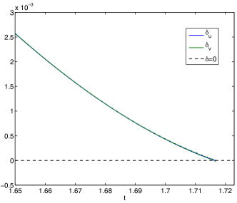
Fig. 1: Fitting parameters $\delta_{u}$ and $\delta_{v}$ corresponding to the fitting to (23) of the Fourier coefficients of $u$ and $v$ respectively. Here $u$ and $v$ are the solution to the 1d hyperbolic dispersionless Toda equation (6) with $\rho=1$ for initial data of the form (25).

To test the influence of resolution in Fourier space on the found results, we present in Fig. 2 the time evolution of $\delta_{u}$ for different resolutions, namely $N=2^{12},2^{13},2^{14},2^{15}$.

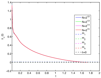
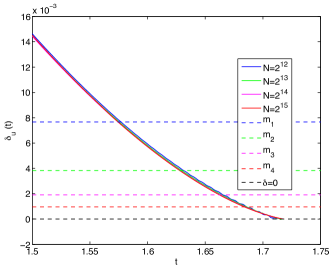
Fig. 2: Fitting parameter $\delta_{u}$ for the solution of the 1d hyperbolic dispersionless Toda equation (6) with $\rho=1$ for initial data of the form 25. The fitting is done for $10<k<2*max(k)/3$ for different resolutions $N=2^{12},2^{13},2^{14},2^{15}$. The figure on the right shows a close-up of the left figure for $t\sim t_{c}$.

In the figure, $m_{i}$ denotes the minimal distance (24) in physical space for a given resolution, $m_{i}=10\pi/N_{i},i=1,2,3,4$ corresponding to $N=2^{12},2^{13},2^{14},2^{15}$. As discussed in [42], the computation can be stopped once $\delta_{u}$ vanishes in the case of a cubic singularity as expected here. Visibly the dispersionless Toda equation behaves as the Hopf equation, i.e., its solutions develop a cubic shock. As observed before, the vanishing of $\delta_{u}$ occurs at $t_{c}\sim 1.717$. At this time, the solution $u$ has indeed a cubic shock, as can seen in Fig. 3, where we present $u$ at several times.

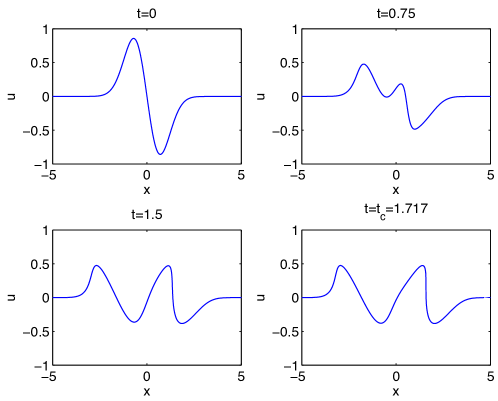
Fig. 3: Solution $u$ of the 1d hyperbolic dispersionless Toda equation (6) with $\rho=1$ at different times for initial data of the form (25).

As was shown in [41, 42], the numerical approach based on asymptotic Fourier analysis is very efficient in the case of a cubic singularity, and the fitting parameter $B_{u}$ converges to the theoretical value ($4/3$) as $N$ increases. This indicates that the fitting is reliable. Moreover, we are able to determine also the location of the singularity as $x_{c}=1.5808$ in the present example. It can be seen from Fig. 4 that $v$ as well has a cubic singularity at $t=t_{c}$.

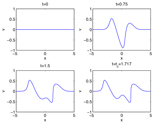
Fig. 4: Solution $v$ of the 1d hyperbolic dispersionless Toda equation (6) with $\rho=1$ at different times for initial data of the form (25).

This can be also obtained from the fitting of the Fourier coefficients $vf$. It had been noted that $\delta_{v}$ vanishes at the same time as $\delta_{u}$, moreover the values of $B_{u}$ and $B_{v}$ are almost identical ($\sim 1.34$), indicating shock formation at the critical time, $t_{c}=1.717$.

We present in Table 1 the values of $t_{c}$, $B_{u}(t_{c})$ and $B_{v}(t_{c})$ for each resolution used. As $N$ increases, $B_{u}(t_{c})$ respectively $B_{v}(t_{c})$ approach $4/3$.

$N$	$t_{c}$	$B_{u}(t_{c})$	$B_{v}(t_{c})$
$2^{12}$	1.7121	1.3518	1.3570
$2^{13}$	1.7157	1.3515	1.3447
$2^{14}$	1.7166	1.3473	1.3488
$2^{15}$	1.7175	1.3461	1.3440

Table 1: Critical times of the solution to the 1d hyperbolic dispersionless Toda equation for initial data of the form (25) for several values of $N$. The values of the fitting parameters $B_{u}$, $B_{v}$ at $t_{c}$ are also given.

As expected, at $t_{c}=1.717$ the gradients of both $u$ and $v$ blow up, with $\|u_{x}\|_{\infty}\sim 70$ and $\|v_{x}\|_{\infty}\sim 95$, see Fig. 5 for the profiles of $|u_{x}|$ and $|v_{x}|$ at the critical time.

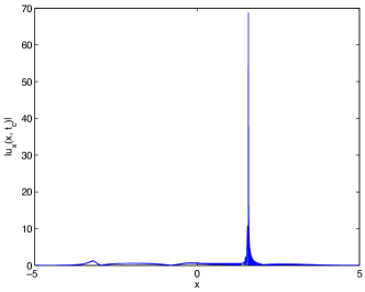
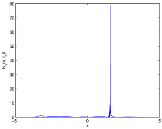
Fig. 5: Profile of $|u_{x}|$ on the left, and of $|v_{x}|$ on the right, at $t=t_{c}=1.717$ for $(u,v)$ being the solution of the 1d hyperbolic dispersionless Toda equation (6) with $\rho=1$ for initial data of the form (25).

We ensure the system is numerically well resolved by checking the decay of the Fourier coefficients during the whole computation, see Fig. 6; the situation for $uf$ is shown on the left, and for $vf$ on the right. Moreover the time evolution of the numerically computed energy does not show any sudden changes, and reaches a value of $\Delta_{E}\sim 10^{-10}$ at the end of the computation at $t=t_{c}$.

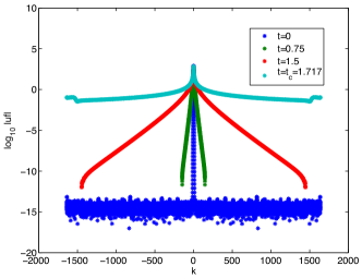
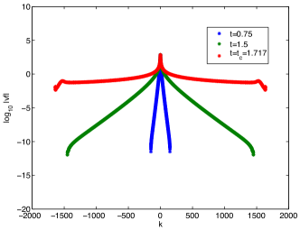
Fig. 6: Fourier coefficients $uf$ of $u$ (left) and $vf$ of $v$ (right) at different times corresponding to the situations in Fig. 3 and 4.

The solutions of the one-dimensional hyperbolic dispersionless Toda equation thus behave like solutions to the Hopf equation for localized initial data, i.e., they develop a cubic shock.

3.2 One-dimensional hyperbolic Toda equation in the limit of small dispersion

In this subsection we study solutions to the one-dimensional hyperbolic Toda equation (4) ($\rho=1$) for small nonzero $\epsilon$. We choose as before the initial data (25) and a time step $\delta_{t}=3*10^{-4}$.

First we study the scaling with $\epsilon$ of the $L_{\infty}$ norm of the difference between the solution to the 1d dispersionless Toda equation (6) and the Toda equation (4) for small $\epsilon$ for the same initial data at the critical time of the former, here at $t_{c}=1.717$. The $L_{\infty}$ norm $\Delta_{\infty}$ of this difference is shown in Fig. 7 at $t_{c}=1.717$ in dependence of $\epsilon$ for $0.02\leq\epsilon\leq 0.1$.

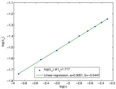
Fig. 7: $L_{\infty}$ norm $\Delta_{\infty}$ of the difference between 1d hyperbolic dispersionless Toda and 1d Toda solutions for the initial data (25) in dependence of $\epsilon$ at $t_{c}=1.717$ for several values of $\epsilon$.

A linear regression analysis ($\log_{10}\Delta_{\infty}=a\log_{10}\epsilon+b$ ) shows that $\Delta_{\infty}$ decreases as

$$\mathcal{O}\left(\epsilon^{0.30}\right)\sim\mathcal{O}\left(\epsilon^{2/7}\right)\,\,\mbox{at}\,\,t=t_{c}=1.717,\,\,\mbox{with}\,\,a=0.3051\,\,\mbox{and}\,\,b=-0.5441.$$ (26)

The correlation coefficient is $r=0.999$. It is thus again similar to the results for the KdV equation and for the defocusing cubic NLS equation in [19].

For larger times and $\epsilon=0.1$ we observe as expected the development of rapid oscillations from $t\sim t_{c}=1.717$ where the solution to the corresponding dispersionless system becomes singular, see Fig. 8 for $u$ and Fig. 9 for $v$.

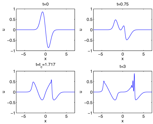
Fig. 8: Solution $u$ of the 1d hyperbolic Toda equation (4) with $\rho=1$ at different times for initial data of the form (25) and $\epsilon=0.1$.

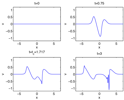
Fig. 9: Solution $v$ of the 1d hyperbolic Toda equation (4) with $\rho=1$ at different times for initial data of the form (25) and $\epsilon=0.1$.

We show in Fig. 10 the corresponding Fourier coefficients at several times. They decrease to machine precision $\sim 10^{-15}$ during the whole computation. In addition the numerically computed energy reaches also the same precision $\Delta_{E}\sim 10^{-15}$ until the maximal time of computation $t_{max}=3$, indicating that the system is well resolved, and that sufficient resolution is provided both in space and in time.

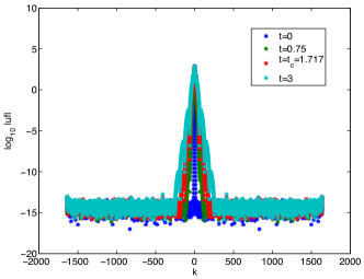
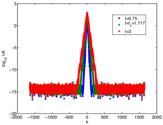
Fig. 10: Fourier coefficients of $u$ (left) and of $v$, (right) at different times, corresponding to the situations in Fig. 8 and 9.

We have identified in the previous subsection the time where the first shock occurs ($t_{c}\sim 1.717$), but we can infer from Fig. 8 and Fig. 9 that a second shock occurs at a later time $t\sim 3$ for negative $x$. It can be observed there that small oscillations begin to form in the region $x<0$.

As $\epsilon\to 0$, the number of oscillations increases as expected as can be seen in Fig. 11 for $u$; the situation is similar for $v$ which is therefore not shown.

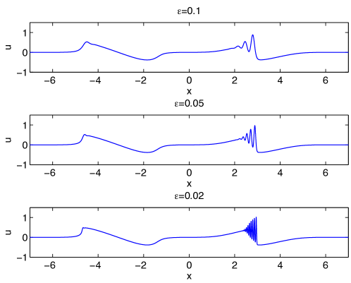
Fig. 11: Solution $u$ of the 1d hyperbolic Toda equation at $t=3$ for different values of $\epsilon$.

3.3 Hyperbolic dispersionless Toda equation in $2+1$ dimensions

We now perform the same study as in the $1+1$ dimensional case in $2+1$ dimensions. We consider initial data of the form

$$u(x,y,0)=u_{0}(x,y)=\partial_{x}\exp(-R^{2}),\,\,R=\sqrt{x^{2}+y^{2}},\,\,\,v(x,y,0)=v_{0}(x,y)=0.$$ (27)

for (10) corresponding to

$$U(x,y,0)=U_{0}(x,y)=\exp(-R^{2}),\,\,R=\sqrt{x^{2}+y^{2}},\,\,\,v(x,y,0)=v_{0}(x,y)=0$$ (28)

for (15). The computations are carried out with $2^{14}\times 2^{9}$ points for $x\times y\in[-5\pi,5\pi]\times[-5\pi,5\pi]$ and time step $\delta_{t}=4*10^{-4}$. We find that the solutions will develop in $x$-direction a singularity as in the $1+1$-dimensional case, but that they stay smooth in $y$-direction. The results described here are thus similar to the ones of [42] for the defocusing semiclassical DS II system.

We will first identify numerically the appearance of break-up in solutions to the 2d dispersionless Toda equations (10) for the initial data (27) for $\rho=1$. The numerical study of the asymptotics of the Fourier coefficients of the resulting solution $u$ leads to a vanishing of the quantity $\delta$ in (22) for $u$, denoted by $\delta_{u}$, at $t=t_{c}=2.162$, see Fig. 12.

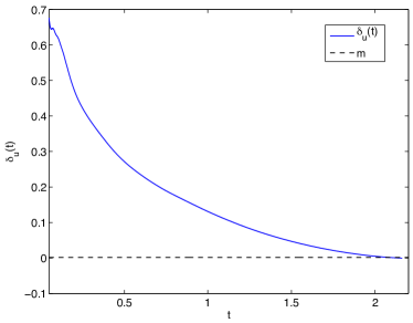
Fig. 12: Fitting parameter $\delta$ in (23) for the solution $u$ (denoted by $\delta_{u}$) of the two-dimensional hyperbolic dispersionless Toda equation (10) with $\rho=1$ for initial data of the form (27). The fitting is done for $10<k<2*max(k)/3$.

At this time the solution develops a shock in $x$-direction as in the $1+1$ dimensional case as can be seen in Fig. 13 where we show the solution ($u,v$) at $t=t_{c}=2.162$.

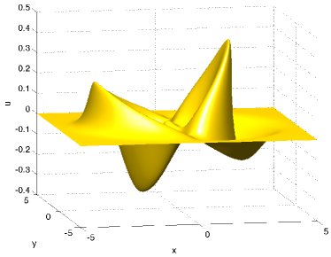
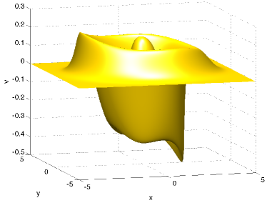
Fig. 13: Solution of the $2+1$ dimensional dispersionless hyperbolic Toda equation (10) with $\rho=1$ for initial data of the form (27) at $t=t_{c}=2.162$.

The cubic singularity can be also inferred from the value of the fitting parameter $B_{u}$ at this time, which reaches a value of $B_{u}(t_{c})=1.353$. We get here less precision than in the one dimensional case (exactly as in the cases reported in [41]) because of the lower space resolution used. The latter is however high enough in terms of accuracy as can be seen in Fig. 14 from the Fourier coefficients of $U$ at several times plotted on the $k_{x}$-axis on the left, and on the $k_{y}$-axis on the right. It can be seen that the chosen resolution for the $y$-direction allows to reach machine precision. In the $x$-direction, i.e., the direction, where the gradient catastrophe occurs, the Fourier coefficients show the expected algebraic decay at $t=t_{c}$.

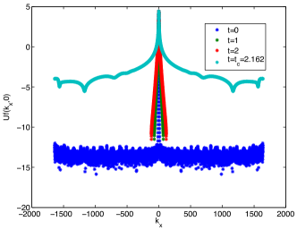
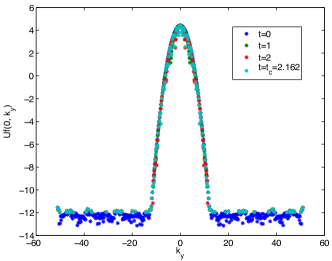
Fig. 14: Fourier coefficients of the solution $U$ of the $2+1$ dimensional hyperbolic dispersionless Toda equation (15) with $\rho=1$ for initial data of the form (28) at several times plotted on the $k_{x}$-axis on the left and on the $k_{y}$-axis on the right.

The numerically computed energy $\Delta_{E}$, where $E$ is defined in (16) reaches a precision of $\sim 10^{-11}$ at the end of the computation, where the $x$-derivative of $u$ begins to blow up, see Fig. 15, with $\|u_{x}\|_{\infty}\sim 50$. In the same way one gets for $|v_{x}|$ that $\|v_{x}\|_{\infty}\sim 65$. The shock is clearly a one-dimensional phenomenon. It can be seen in Fig. 15 that $u_{y}$ stays small, with $\|u_{y}\|_{\infty}\sim 2$. The location of the singularity is found to be $\alpha(t_{c})=2.2615$ on the $x$-axis.

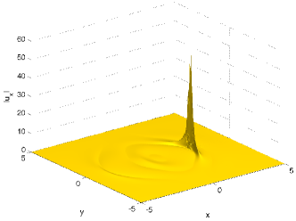
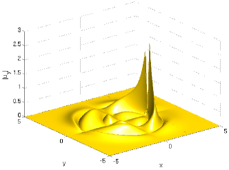
Fig. 15: Absolute value of the $x$-derivative of $u$ of Fig. 13 at $t=t_{c}=2.162$ on the left, and of the $y$-derivative on the right.

3.4 Small dispersion limit of the hyperbolic Toda equation in $2+1$ dimensions

In this subsection we study the solutions for the hyperbolic Toda equation in $2+1$ dimensions (4) for the initial data (28) for small nonzero $\epsilon$.

First we investigate the scaling with $\epsilon$ of the $L_{\infty}$ norm $\Delta_{\infty}$ of the difference between the solutions to the 2d dispersionless Toda (10) and the Toda (9) equation for the same initial data in dependence of $\epsilon$. The $L_{\infty}$ norm of this difference is shown in Fig. 16 at $t_{c}=2.162$ for $0.01\leq\epsilon\leq 0.1$.

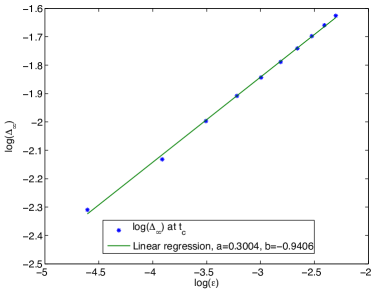
Fig. 16: $L_{\infty}$ norm $\Delta_{\infty}$ of the difference between solutions to the 2d hyperbolic dispersionless Toda and the Toda equation for the initial data (27) in dependence of $\epsilon$ at $t_{c}=2.162$.

A linear regression analysis ($\log_{10}\Delta_{\infty}=a\log_{10}\epsilon+b$ ) shows that $\Delta_{\infty}$ decreases as

$$\mathcal{O}\left(\epsilon^{0.30}\right)\sim\mathcal{O}\left(\epsilon^{2/7}\right)\,\,\mbox{at}\,\,t=t_{c}=2.162,\,\,\mbox{with}\,\,a=0.3004\,\,\mbox{and}\,\,b=-0.9406.$$ (29)

The correlation coefficient is $r=0.99$. As expected, the situation is similar to the $1+1$ dimensional case which itself is as for KdV and the defocusing NLS equation.

For $t\gg t_{c}$ the solution of the hyperbolic Toda equation in $2+1$ dimensions (9) with $\rho=1$ for initial data of the form (27) develops as expected a zone of rapid modulated oscillations, where the solution of the corresponding dispersionless system admits a shock (as identified in the previous subsection). We show the numerical solution $u$ of (9) with $\epsilon=0.1$ in Fig. 17 and $v$ in Fig. 18 at several times.

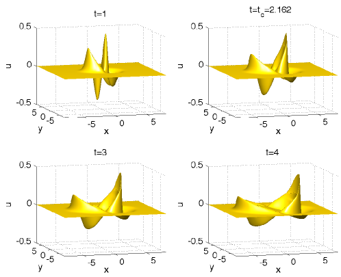
Fig. 17: Solution $u$ of the $2+1$ dimensional hyperbolic Toda equation (9) with $\rho=1$ at different times for initial data of the form (27) and $\epsilon=0.1$.

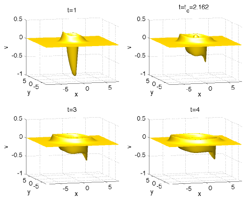
Fig. 18: Solution $v$ of the $2+1$ dimensional hyperbolic Toda equation (9) with $\rho=1$ at different times for initial data of the form (27) and $\epsilon=0.1$.

The Fourier coefficients decrease to machine precision during the whole computation in both spatial directions. As an example, we show in Fig. 19 the Fourier coefficients of $u$ on the left and of $v$ on the right plotted on the $k_{x}$-axis at different times.

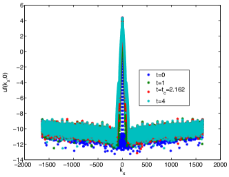
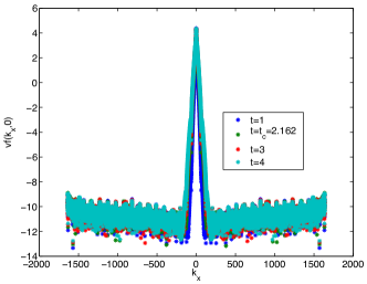
Fig. 19: Fourier coefficients of $u$ (left) and of $v$ (right) on the $k_{x}$-axis at different times, corresponding to the situations in Fig. 17 and 18.

As $\epsilon$ becomes smaller, the number of oscillations increases as can be seen in Fig. 20 for $u$ and in Fig. 21 for $v$.

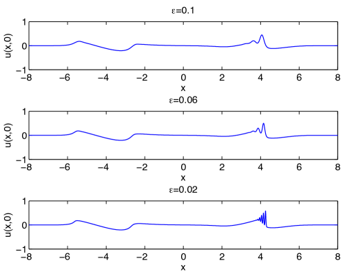
Fig. 20: Solutions $u$ of the $2+1$ dimensional hyperbolic Toda equation (9) with $\rho=1$ at $t=4$ on the $x$-axis for different values of $\epsilon$.

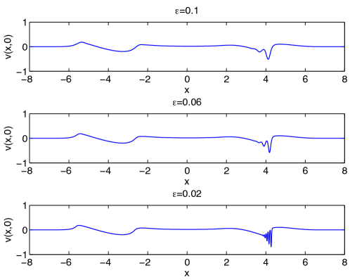
Fig. 21: Solutions $v$ of the $2+1$ dimensional hyperbolic Toda equation (9) with $\rho=1$ at $t=4$ on the $x$-axis for different values of $\epsilon$

The contour plots of the solutions $u$ at $t=4$ of (9) with $\rho=1$ for several values of $\epsilon$ can be seen in Fig. 22. Note again the formation of an oscillatory zone which becomes more clearly delimited for smaller $\epsilon$.

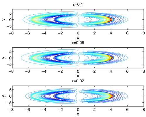
Fig. 22: Contour plot of the solutions $u$ of the $2+1$ dimensional hyperbolic Toda (9) with $\rho=1$ equation at $t=4$ for different values of $\epsilon$.

4 Numerical study of the elliptic Toda equations

In this section we study the small dispersion limit of the elliptic Toda equations in $1+1$ and $2+1$ dimensions for the same initial data as in the hyperbolic case. We find for the one-dimensional dispersionless system that a cusp forms as in the case of the focusing semiclassical Schrödinger equations in $1+1$ dimensions. For small nonzero $\epsilon$ this cusp is not regularized via a dispersive shock as in the hyperbolic case, but leads to an $L_{\infty}$ blow-up in finite time $t^{*}>t_{c}$. The situation is thus as in the semiclassical limit of NLS equations with critical or supercritical nonlinearity. In $2+1$ dimensions the situation is similar to what was observed for the focusing DS II equations in [42]. Concretely we find:

• the solution to the dispersionless equation has a point of gradient catastrophe on the $x$-axis of square root type, whereas it stays regular in $y$-direction;

• the difference between the solutions to the dispersionless and the full Toda equation scales as $\epsilon^{2/5}$ as in the one-dimensional case;

• for times larger than $t_{c}$, the solution develops for $\epsilon\ll 1$ an $L_{\infty}$ blow-up in finite time $t^{*}>t_{c}$.

The scaling of the difference between the solutions to the dispersionless and the full Toda equation for small $\epsilon$ as $\epsilon^{2/5}$ could indicate that the tritronquée solution of the PI equation might play a role also in the asymptotic description of the Toda solution near the break-up of the corresponding solution to the dispersionless equation.

4.1 Dispersionless elliptic Toda equation in $1+1$ dimensions

In this subsection we study again the initial data (25), but this time for equation (6) with $\rho=-1$. The Fourier coefficients for the solution are fitted to the asymptotic formula (23). It was shown at the example of exact solutions for the semiclassical NLS equations in $1+1$ dimensions in [42] that for elliptic systems, the break-up is best identified from the asymptotic behavior of the Fourier coefficients if the code is stopped once the $\delta$ in (22) becomes smaller than the smallest resolved distance (24) in physical space. Since we deal with an elliptic system here as well, we use the same criterion as in [42] to identify the formation of a singularity.

To solve the dispersionless Toda equation (6) with $\rho=-1$ for the initial data (25), we use $N=2^{14}$ Fourier modes and the time step $\delta_{t}=5*10^{-5}$. The resulting solutions $u$ and $v$ are shown for several times up to the critical time $t_{c}$ in Fig. 23, respectively 24. The former clearly develops a cusp, as in the case of the focusing semiclassical NLS equation. As in the latter case in [42], we get a value of $B_{u}$ close to one instead of the expected value $1.5$. The reason for this is again that the quantity $B=\mu+1$ in (23), corresponding to an algebraic decrease of the Fourier coefficients, is much more sensitive to the fitting procedure than the exponential part parametrized by $\delta$. Thus the errors in the Fourier coefficients for the high wave numbers as discussed in [42] affect the determination of $\mu$ much more than the vanishing of $\delta$.

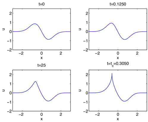
Fig. 23: Solution $u$ of the 1d elliptic dispersionless Toda equation (6) with $\rho=-1$ at different times for initial data of the form (25).

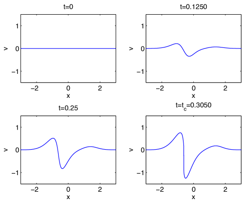
Fig. 24: Solution $v$ of the 1d elliptic dispersionless Toda equation (6) with $\rho=-1$ at different times for initial data of the form (25).

The behavior of $|u_{x}|$ and $|v_{x}|$ at $t=t_{c}=0.3050$ is shown in Fig. 25. We observe at this time that $\|u_{x}\|_{\infty}\sim 45$ and $\|v_{x}\|_{\infty}\sim 230$ which clearly indicates a point of gradient catastrophe for both $u$ and $v$.

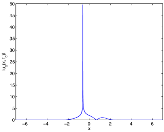
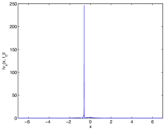
Fig. 25: Gradient of $u$ on the left and of $v$ on the right at the critical time $t_{c}=0.3050$; $(u,v)$ being the solution of the 1d elliptic dispersionless Toda equation (6) with $\rho=-1$ for initial data of the form (25).

To control the accuracy of the solution, we present in Fig. 26 the Fourier coefficients for the situation in Fig. 23 and 24. We also verify that the numerically computed energy reaches a precision of $\Delta_{E}\sim 10^{-13}$ at $t=t_{c}=0.305$.

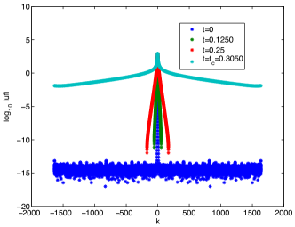
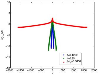
Fig. 26: Fourier coefficients of $u$ (left), denoted by $uf$, and Fourier coefficients of $v$, denoted respectively by $vf$, at different times, corresponding to the situations in Fig. 23 and 24.

Since the determination of the critical point and the critical solution is crucial for the understanding of the behavior of the solution to the full Toda equation in the vicinity of the critical point, we discuss the used approach in more detail. In Fig. 27, we show the time evolution of $\delta_{u}$ (the parameter $\delta$ in (22) for $u$) for different resolutions $N$. We perform the fitting for the same range of $k$ as in the hyperbolic case, but stop the computation when $\delta_{u}$, respectively $\delta_{v}$ are smaller than the smallest distance $m$ (24) resolved in physical space.

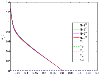
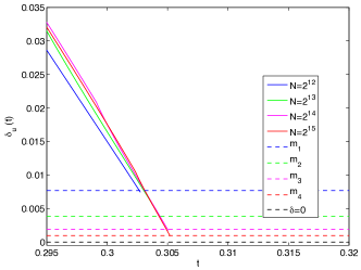
Fig. 27: Fitting parameter $\delta$ in (23) for $u$ (denoted by $\delta_{u}$) for the solution of the 1d elliptic dispersionless Toda equation (6) with $\rho=-1$ for initial data of the form (25). The fitting is done for $10<k<2*max(k)/3$ for different resolutions $N=2^{12},2^{13},2^{14},2^{15}$; on the right a close-up of the situation for $t\sim t_{c}$.

As already observed in the previous section, both the fitting of the Fourier coefficients $uf$ and on $vf$ give (within numerical precision) the same critical time, $t_{c}\sim 0.305$ as shown in Table 2, which indicates the consistency and the reliability of the approach. In Table 2 we also present the corresponding values of $B_{u}(t_{c})$ and $B_{v}(t_{c})$ which are, as expected in [42], not close to the expected 1.5. Note that the found critical times for $N=2^{14}$ and $N=2^{15}$ are almost identical which means that a resolution of $N=2^{14}$ points is sufficient for our purposes.

$N$	$t_{c}$	$B_{u}(t_{c})$	$B_{v}(t_{c})$
$2^{12}$	0.3027	1.2204	1.1349
$2^{13}$	0.3044	1.1172	1.0365
$2^{14}$	0.3050	1.0575	0.9785
$2^{15}$	0.3052	1.0193	0.9424

Table 2: Critical times of the solution to the 1d elliptic dispersionless Toda equation for initial data of the form (25) for several values of $N$. The values of the fitting parameters $B_{u}$, $B_{v}$ at $t_{c}$ are also given.

Thus we find here that the solutions of the elliptic dispersionless Toda equation in $1+1$ dimensions show a very similar behavior to what was found in [42] for the semiclassical cubic NLS equation. This indicates that the singularity is in both cases of square root type.

4.2 One-dimensional elliptic Toda equation in the limit of small dispersion

In this subsection, we study the behavior of solutions of the $1+1$ dimensional Toda equation (4) for several small values of $\epsilon$ and initial data of the form (25). The solutions will be compared near the critical time $t_{c}$ with the critical solution of the dispersionless system (6) for the same initial data.

We compute the solution to the elliptic Toda equation (4) with $\rho=-1$ for different values of $\epsilon$ for initial data of the form (25). The computation is carried out with $N=2^{14}$ points for $x\in[-5\pi,5\pi]$ and time step $\Delta_{t}=5*10^{-5}$. We first study the solution up to the critical time of the corresponding dispersionless system determined in the previous subsection, i.e., $t_{c}=0.3050$.

We are interested in the scaling in $\epsilon$ of the $L_{\infty}$ norm $\Delta_{\infty}$ of the difference between the solutions to the 1d elliptic dispersionless Toda and the full Toda equation for the same initial data (25). This norm is shown in Fig. 28 at $t_{c}=0.3050$ for $0.01\leq\epsilon\leq 0.1$.

Fig. 28: $L_{\infty}$ norm $\Delta_{\infty}$ of the difference between solutions to the 1d elliptic dispersionless Toda and the Toda equation for the initial data (25) in dependence of $\epsilon$ at $t_{c}=0.3050$.

A linear regression analysis ($\log_{10}\Delta_{\infty}=a\log_{10}\epsilon+b$ ) shows that $\Delta_{\infty}$ decreases as

$$\mathcal{O}\left(\epsilon^{0.40}\right)\sim\mathcal{O}\left(\epsilon^{2/5}\right)\,\,\mbox{at}\,\,t=t_{c}=0.3050,\,\,\mbox{with}\,\,a=0.4005\,\,\mbox{and}\,\,b=0.3751.$$ (30)

The correlation coefficient is $r=0.999$. Thus we find the same scaling as conjectured for NLS equations, see [17, 19].

For times greater than $t_{c}$, we find as in the case of the $1+1$ dispersionless quintic (or higher power nonlinearity) NLS equation that the solution blows up in finite time. We use again the asymptotics of the Fourier coefficients (23) to determine the time of the appearance of a singularity on the real axis as in [42, 49]. As the blow-up time $t^{*}$ we define the time when the quantity $\delta$ in (23) for $u$ (denoted by $\delta_{u}$) becomes smaller than the smallest resolved distance (24) in physical space. In Fig. 29 we show the time evolution of $\delta_{u}$ for several values of $\epsilon$.

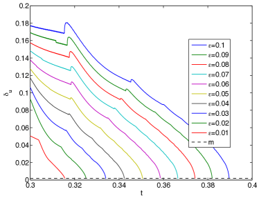
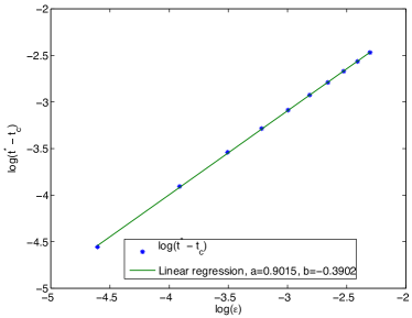
Fig. 29: Fitting parameter $\delta$ of (22) for the solution $u$ (denoted by $\delta_{u}$) of the 1d elliptic Toda equation (4) with $\rho=-1$ for initial data of the form 25 on the left, and the $L_{\infty}$ norm of the difference between blow-up time $t^{*}$ and break-up time $t_{c}$ in dependence of $\epsilon$ on the right in a loglog plot.

The thus determined blow-up times $t^{*}$ are given in Table 3 for different values of $\epsilon$. The $L_{\infty}$ norm of the difference $t^{*}-t_{c}$ scales as $\epsilon^{0.9}$, see Fig. 29 where the results of the linear regression are shown.

$\epsilon$	$0.1$	$0.09$	$0.08$	$0.07$	$0.06$	$0.05$	$0.04$	$0.03$	$0.02$	$0.01$
$t^{*}$	0.3896	0.3819	0.3742	0.3664	0.3586	0.3506	0.3424	0.3340	0.3251	0.3155

Table 3: Values of the determined blow-up times of the solution of the 1d elliptic Toda equation (4) with $\rho=-1$ for initial data of the form (25) for several values of $\epsilon$.

Thus as for focusing NLS equations, we find here that in the limit of small dispersion, i.e., as $\epsilon\to 0$, the solutions to the Toda equation (4) blow up in the $L_{\infty}$ norm at a finite time $t^{*}$. This time is always greater than the critical time of the break-up of the corresponding solution to the dispersionless system. In the limit $\epsilon\to 0$, the blow-up time tends to the break-up time roughly as $\epsilon^{0.9}$.

4.3 Dispersionless elliptic two-dimensional Toda equation

In this subsection we numerically solve the dispersionless elliptic Toda equation (10) in $2+1$ dimensions for the initial data (27). It is shown that the same type of singularity is found as in the $1+1$ dimensional case.

For the dispersionless $2+1$ dimensional Toda equation (10) with $\rho=-1$, we use $2^{14}\times 2^{9}$ points for $x\times y\in[-5\pi,5\pi]\times[-5\pi,5\pi]$ and the time step is $\delta_{t}=5*10^{-5}$. We find that the solution of the dispersionless system for initial data of the form (27) develops a singularity at $t_{c}\sim 0.3007$. As in the $1+1$ dimensional case, the latter time is obtained from the asymptotic behavior of the Fourier coefficients: the Fourier coefficients for $u$ are fitted to the asymptotic formula (23) giving $\delta_{u}$. The critical time is defined as the time when $\delta_{u}$ becomes smaller than the smallest resolved distance (24) in physical space, see Fig. 30.

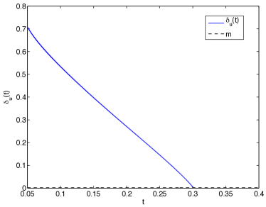
Fig. 30: Fitting parameter $\delta$ in (22) for $u$ (denoted by $\delta_{u}$) for the solution of the two-dimensional elliptic dispersionless Toda equation (10) with $\rho=-1$ for initial data of the form (27). The fitting is done for $10<k<2*max(k)/3$.

The solutions $u$ and $v$ at $t_{c}=0.3007$ can be seen in Fig. 31. Visibly $u$ develops a cusp in $x$-direction as in the one-dimensional case.

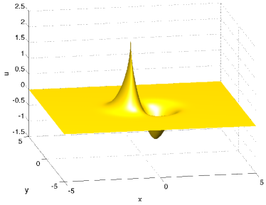
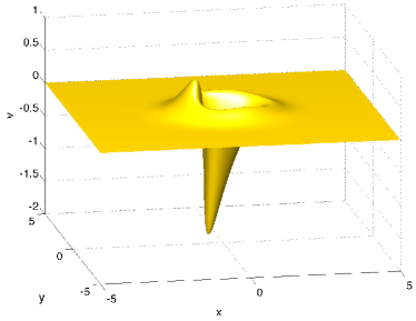
Fig. 31: Solutions $u$ and $v$ of the elliptic dispersionless Toda equation in $2+1$ dimensions (10) with $\rho=-1$ at $t=t_{c}=0.3007$ for initial data of the form (27).

The $x$ derivatives of the solution diverge as can be seen from the behavior of $|u_{x}|$ and $|v_{x}|$ at $t=t_{c}=0.3007$ in Fig. 32. We observe at this time that $\|u_{x}\|_{\infty}\sim 60$ and $\|v_{x}\|_{\infty}\sim 280$.

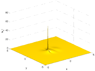
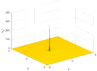
Fig. 32: $x$ derivative of $u$ on the left, and of $v$ on the right, at $t=t_{c}=0.3007$; $(u,v)$ being the solution of the $2+1$ dimensional elliptic dispersionless Toda equation (10) with $\rho=-1$ for initial data of the form (27).

The singularity is one-dimensional, one finds that the $y$-derivatives of $u$ and $v$ remain small at the critical time, see Fig. 33.

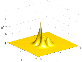
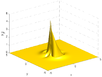
Fig. 33: $y$ derivative of $u$ on the left, and of $v$ on the right, at $t=t_{c}=0.3007$; $(u,v)$ being the solution of the $2+1$ dimensional elliptic dispersionless Toda equation (10) with $\rho=-1$ for initial data of the form (27).

To ensure the accuracy of the numerical solution, we again consider the Fourier coefficients of $u$ in Fig. 34 at several times. It can be seen that the solution is numerically well resolved up to the formation of the singularity.

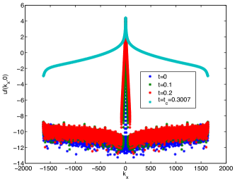
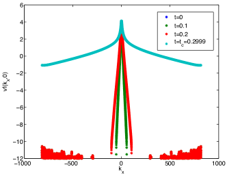
Fig. 34: Fourier coefficients of $u$ (left), denoted by $uf$, and of $v$ (right), denoted by $vf$, plotted on the $k_{x}$-axis at different times corresponding to the situation in Fig. 31.

4.4 Small dispersion limit of the elliptic two-dimensional Toda equation

In this subsection we numerically solve the $2+1$ dimensional elliptic Toda equation for the initial data (27) for small nonzero $\epsilon$. We show that the difference between the solution to the 2d dispersionless Toda equation and the Toda equation with small $\epsilon$ scales as in the $1+1$ dimensional case as $\epsilon^{2/5}$ at the critical time $t_{c}$. This is the same behavior as found for the focusing DS II equation in [42]. For times larger than $t_{c}$, we find as in the $1+1$ dimensional case an $L_{\infty}$ blow-up.

We compute the solution to the elliptic Toda equation (9) with $\rho=-1$ for different values of $\epsilon$ with $2^{14}\times 2^{9}$ points for $x\times y\in[-5\pi,5\pi]\times[-5\pi,5\pi]$ and time step $\delta_{t}=5*10^{-5}$. We first study the solution until the critical time $t_{c}=0.3007$ of the corresponding dispersionless system. We are interested in the scaling in $\epsilon$ of the $L_{\infty}$ norm $\Delta_{\infty}$ of the difference between the solution to the 2d elliptic dispersionless Toda equation (10) and the Toda equation (9) for the same initial data (27). This difference is shown in Fig. 35 at $t_{c}=0.3007$ for $0.01\leq\epsilon\leq 0.1$.

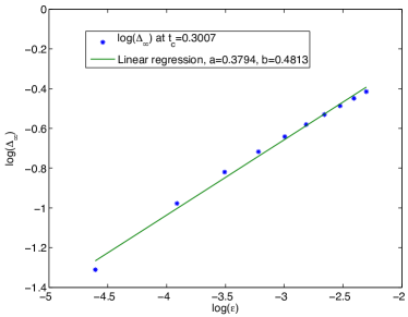
Fig. 35: $L_{\infty}$ norm $\Delta_{\infty}$ of the difference between the solutions to $2+1$ dimensional elliptic dispersionless Toda and the Toda equation for the initial data (27) in dependence of $\epsilon$ at $t_{c}=0.3007$.

A linear regression analysis ($\log_{10}\Delta_{\infty}=a\log_{10}\epsilon+b$ ) shows that $\Delta_{\infty}$ decreases as

$$\mathcal{O}\left(\epsilon^{0.40}\right)\sim\mathcal{O}\left(\epsilon^{2/5}\right)\,\,\mbox{at}\,\,t=t_{c}=0.3007,\,\,\mbox{with}\,\,a=0.3794\,\,\mbox{and}\,\,b=0.4813.$$ (31)

The correlation coefficient is $r=0.999$.

For times $t>t_{c}$ we find as in the $1+1$ dimensional case that the solution blows up in finite time. Again we use the asymptotic analysis of the Fourier coefficients to obtain the blow-up time $t^{*}$ as the time when $\delta_{u}$ (the $\delta$ in (22) for $u$) becomes smaller than the smallest resolved distance in physical space (24). In Fig. 36 we show the time evolution of $\delta_{u}$ for several values of $\epsilon$.

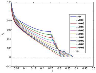
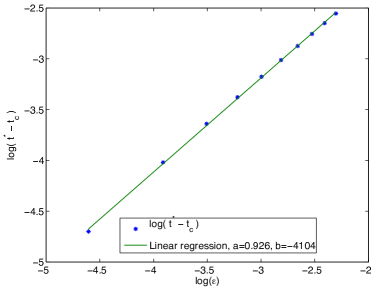
Fig. 36: Fitting parameter $\delta_{u}$ (the $\delta$ in (22) for $u$) for the solution of the $2+1$ dimensional elliptic Toda equation (9) with $\rho=-1$ with initial data of the form 27 on the left, and the $L_{\infty}$ norm of the difference between blow-up time $t^{*}$ and break-up time $t_{c}$ in dependence of $\epsilon$ on the right in a loglog plot.

The thus determined blow-up times $t^{*}$ are given in Table 4 for different values of $\epsilon$. The $L_{\infty}$ norm of $(t^{*}-t_{c})$ shows a scaling with $\epsilon$ of the form $\epsilon^{0.9}$ as in the $1+1$ dimensional case, see Fig. 36.

$\epsilon$	$0.1$	$0.09$	$0.08$	$0.07$	$0.06$	$0.05$	$0.04$	$0.03$	$0.02$	$0.01$
$t^{*}_{\epsilon}$	0.3785	0.3714	0.3643	0.3572	0.3498	0.3424	0.3348	0.3270	0.3186	0.3098

Table 4: Values of the determined blow-up times of the solutions to the 2d elliptic Toda equation (9) with $\rho=-1$ for initial data of the form (27) for several values of $\epsilon$.

5 Outlook

In this paper we have studied numerically the Toda equations in $1+1$ and $2+1$ dimensions. The goal was to investigate various critical regimes of the equations, especially the continuum limit. It was shown that the used numerical tools are able also to address the formation of singularities in a reliable way. This allowed to identify break-up and blow-up in solutions to these equations and even to identify the scaling of the solutions in critical parameters in the vicinity of critical points.

We concentrated here on the completely integrable Toda system since the numerical results were intended to encourage analytical efforts to prove or enhance the found conjectures. Since this is most likely for integrable systems for which powerful analytical methods as RHPs exist, we only considered integrable cases. The used numerical techniques are, however, in no way limited to integrable systems. It is the goal of further research to explore not integrable FPU models and address similar questions as for Toda in this paper. As in [18] for the generalized KdV equation, an interesting issue will be to explore to which extent the found features here are universal also for non-integrable systems, or how they will change if the studied system is not close to integrability.

References

- [1] D. Bambusi, T. Kappeler, and T. Paul. From Toda to KdV. arXiv:1309.5324, 2013.
- [2] D. Bambusi and A. Ponno. On metastability in FPU. Comm. Math. Phys., 264(2):539–561, 2006.
- [3] G. Benettin, R. Livi, and A. Ponno. The Fermi-Pasta-Ulam problem: scaling laws vs. initial conditions. Journ. Stat. Phys., 135:873–893, 2009.
- [4] P. Boutroux. Recherches sur les transcendants de M. Painlevé et l’étude asymptotique des équations différentielles du second ordre. Ann. Éc. Norm., 30:265–375, 1913.
- [5] C.P. Boyer and J.D. Finley. Killing vectors in self-dual Euclidean Einstein spaces. J. Math. Phys., 23:1126–1130, 1982.
- [6] M.E. Brachet, M. Meneguzzi, and P.-L. Sulem. Numerical simulation of decaying two-dimensional turbulence: comparison between general periodic and Taylor-Green like flows. In Macroscopic modelling of turbulent flows (Nice, 1984), volume 230 of Lecture Notes in Phys., pages 347–355. Springer, Berlin, 1985.
- [7] R.E. Caflisch. Singularity formation for complex solutions of the D incompressible Euler equations. Phys. D, 67(1-3):1–18, 1993.
- [8] D.K. Campbell, P. Rosenau, and G.M. Zaslavsky. The Fermi-Pasta-Ulam problem-The first fifty years. Chaos: An Interdisciplinary Journal of Nonlinear Science, 15, 2005.
- [9] G. Carlet, B.A. Dubrovin, and L.-P. Mertens. Infinite-dimensional Frobenius manifolds for 2 + 1 integrable systems. Matematische Annalen, 349:75–115, 2011.
- [10] L. Casetti, M. Cerruti-Sola, M. Pettini, and E.G.D. Cohen. The Fermi-Pasta-Ulam problem revisited: Stochasticity thresholds in nonlinear Hamiltonian systems. Phys. Rev. E, 55:6566–6574, 1997.
- [11] T. Claeys and T. Grava. Universality of the break-up profile for the KdV equation in the small dispersion limit using the Riemann-Hilbert approach. Comm. Math. Phys., 286:979–1009, 2009.
- [12] T. Claeys and M. Vanlessen. The existence of a real pole-free solution of the fourth order analogue of the Painlevé I equation. Nonlinearity, 20(5):1163–1184, 2007.
- [13] G. Della Rocca, M. C. Lombardo, M. Sammartino, and V. Sciacca. Singularity tracking for Camassa-Holm and Prandtl’s equations. Appl. Numer. Math., 56(8):1108–1122, August 2006.
- [14] W. Dreyer and M. Herrmann. Numerical experiments on the modulation theory for the nonlinear atomic chain. Physica D, 237:255–282, 2008.
- [15] B.A. Dubrovin. On Hamiltonian perturbations of hyperbolic systems of conservation laws, II: universality of critical behaviour. Comm. Math. Phys., 267:117 –139, 2006.
- [16] B.A. Dubrovin. On universality of critical behaviour in Hamiltonian PDEs. Amer. Math. Soc. Transl., 224:59–109, 2008.
- [17] B.A. Dubrovin, T. Grava, and C. Klein. On universality of critical behaviour in the focusing nonlinear Schrödinger equation, elliptic umbilic catastrophe and the tritronquée solution to the Painlevé-I equation. J. Nonl. Sci., 19(1):57–94, 2009.
- [18] B.A. Dubrovin, T. Grava, and C. Klein. Numerical Study of breakup in generalized Korteweg-de Vries and Kawahara equations. SIAM J. Appl. Math., 71:983–1008, 2011.
- [19] B.A. Dubrovin, T. Grava, C. Klein, and A. Moro. On critical behaviour in systems of Hamiltonian PDEs. 2013. preprint.
- [20] M. Dunajski, L.J. Mason, and K.P. Tod. Einstein-Weyl geometry, the dKP equation and twistor theory. J. Geom. Phys., 37:63–92, 2001.
- [21] E. Ferapontov, D. Korotkin, and V. Shramchenko. Boyer-Finley equation and systems of hydrodynamic type. Class. Quant. Grav., 19:L205–L210, 2002.
- [22] W.E. Ferguson, Jr., H. Flaschka, and D.W. McLaughlin. Nonlinear normal modes for the Toda chain. J-COMPUT-PHYS, 45(2):157–209, February 1982.
- [23] E. Fermi, J. Pasta, and S.M. Ulam. Studies in nonlinear problems.Technical Report LA-1940. Los Alamos Scientific Laboratory, pages 977–988, 1955.
- [24] S. Flach and A. Ponno. The Fermi-Pasta-Ulam problem: Periodic orbits, normal forms and resonance overlap criteria. Physica D, 237:908–917, 2008.
- [25] H. Flaschka. The Toda lattice. Phys. Rev. B9, 1974.
- [26] H. Flaschka. The Toda lattice II. Progr. Theor. Phys., 51:703–716, 1974.
- [27] J. Ford. The Fermi-Pasta-Ulam problem: Paradox turns discovery. Physics Reports, 213:271–310, 1992.
- [28] U. Frisch, T. Matsumoto, and J. Bec. Singularities of Euler flow? Not out of the blue! J. Statist. Phys., 113(5-6):761–781, 2003. Progress in statistical hydrodynamics (Santa Fe, NM, 2002).
- [29] G. Gallavotti. The Fermi-Pasta-Ulam Problem: A Status Report, volume 728 of Lect. Notes Phys. Springer-Verlag, 2008.
- [30] F. Gargano, M. Sammartino, and V. Sciacca. Singularity formation for Prandtls equations. Physica D, 238:1975–1991, 2009.
- [31] F. Gargano, M. Sammartino, V. Sciacca, and K.W. Cassel. Analysis of complex singularities in high-Reynolds-number Navier-Stokes solutions. preprint 2013.
- [32] F. Gesztesy, H. Holden, J. Michor, and G. Teschl. Soliton Equations and Their Algebro-Geometric Solutions; Volume II: (1+1)-Dimensional Discrete Models, volume 114 of Cambridge Studies in Adv. Math. Cambridge Univ. Press., Cambridge, 2008.
- [33] A. Giorgilli, S. Paleari, and T. Penati. Local chaotic behaviour in the Fermi-Pasta-Ulam system. DCDS-B, 5(4):991–1004, 2005.
- [34] T. Grava and C. Klein. Numerical study of a multiscale expansion of KdV and Camassa-Holm equation. In J. Baik, T. Kriecherbauer, L.-C. Li, K.D.T-R. McLaughlin, and C. Tomei, editors, Integrable Systems and Random Matrices, volume 458 of Contemp. Math., pages 81–99. 2008.
- [35] S. Isola, R. Livi, S. Ruffo, and A. Vulpiani. Stability and chaos in Hamiltonian dynamics. Pys. Rev A, 33:1163–1170, 1986.
- [36] F. M. Izrailev and B. V. Chirikov. Statistical properties of a nonlinear string. Sov. Phys. Dokl., 11:30–32, 1966.
- [37] A. Kapaev, C. Klein, and T. Grava. On the tritronquée solutions of P. preprint, 2013. Preprint available at: arXiv:1306.6161.
- [38] A-K. Kassam and L.N. Trefethen. Fourth-Order Time-Stepping for stiff PDEs. SIAM J. Sci. Comput, 26(4):1214–1233, 2005.
- [39] C. Klein. Fourth order time-stepping for low dispersion Korteweg-de Vries and nonlinear Schrödinger Equation. Electronic Transactions on Numerical Analysis., 39:116–135, 2008.
- [40] C. Klein and K. Roidot. Fourth order time-stepping for Kadomtsev-Petviashvili and Davey-Stewartson equations. SIAM J. Sci. Comp., 33:DOI: 10.1137/100816663, 2011.
- [41] C. Klein and K. Roidot. Numerical study of shock formation in the dispersionless Kadomtsev-Petviashvili equation and dispersive regularizations. Physica D: Nonlinear Phenomena, 265:1–25, 2013.
- [42] C. Klein and K. Roidot. Numerical Study of the semiclassical limit of the Davey-Stewartson II equations. preprint, 2013. Preprint available at: arXiv:1401.4745.
- [43] C. Klein, C. Sparber, and P. Markowich. Numerical Study of oscillatory Regimes in the Kadomtsev-Petviashvili Equation. Max-Planck-Institut für Mathematik in den Naturwissenschaften Leipzig Preprint N° 124, 2005.
- [44] S.V. Manakov. On the complete integrability and stochastization in discrete dynamical systems. Soviet Physics, JETP, 40:269–274, 1974.
- [45] S.V. Manakov and P.M. Santini. The dispersionless 2D Toda eqation: dressing, Cauchy problem, longtime behaviour, implicit solutions and wave breaking. J.Phys.A:Math.Theor., 42, 2009.
- [46] M. Matsukawa and S. Watanabe. A Transformation connecting the Two dimensional Toda lattice and KdV equation. J. Phys. Soc. Jap., 57, No 8.:2685–2688, 1988.
- [47] T. Matsumoto, J. Bec, and U. Frisch. The analytic structure of 2D Euler flow at short times. Fluid Dynam. Res., 36(4-6):221–237, 2005.
- [48] M. Pugh and M. Shelley. Singularity Formation in thin J with Surface Tension. Comm. Pure Appl. Math., 51:733–795, 1998.
- [49] K. Roidot and N. Mauser. Numerical study of the transverse stability of NLS soliton solutions in several classes of NLS type equations. arXiv1401.5349, 2014.
- [50] N. Saitoh. A Transformation connecting the Toda lattice and the KdV equation. J. Phys. Soc. Jap., 49:409–416, 1980.
- [51] T. Schmelzer. The fast evaluation of matrix functions for exponential integrators. PhD thesis, Oxford University, 2007.
- [52] C. Sulem, P.L. Sulem, and H. Frisch. Tracing complex singularities with spectral methods. J. Comp. Phys., 50:138–161, 1983.
- [53] P.-L. Sulem, C. Sulem, and A. Patera. Numerical simulation of singular solutions to the two-dimensional cubic Schrödinger equation. Comm. Pure Appl. Math., 37(6):755–778, 1984.
- [54] G. Teschl. Jacobi Operators and Complete Integrable Nonlinear Lattices,, volume 72 of Math. Surv. and Mon. Amer. Math. Soc., Rhode Island, 2000.
- [55] M. Toda. Theory of nonlinear lattices, 2nd enl. ed. Springer, Berlin, 1989.
- [56] M. Toda. Theory of nonlinear waves and solitons. Kluwer, Dordrecht, 1989.
- [57] N.J. Zabusky and M.D. Kruskal. Interaction of Solitons in a collisionless Plasma and the Recurrence of initial States. Physics Rev. Lett., 15:240–243, 1965.
- [58] N.J. Zabusky, Z. Sun, and G. Peng. Measures of chaos and equipartition in integrable and nonintegrable lattices. Chaos, 16 013130/:1–12, 2006.