Membranes and Sheaves

1 A brief introduction

1.1 Overview

Our goal in this paper is to discuss a conjectural correspondence between enumerative geometry of curves in Calabi-Yau 5-folds $Z$ and $1$-dimensional sheaves on 3-folds $X$ that are embedded in $Z$ as fixed points of certain $\mathbb{C}^{\times}$-actions. In both cases, the enumerative information is taken in equivariant $K$-theory, where the equivariance is with respect to all automorphisms of the problem.

In Donaldson-Thomas theories, one sums up over all Euler characteristics with a weight $(-q)^{\chi}$, where $q$ is a parameter. Informally, $q$ is referred to as the boxcounting parameter. The main feature of the correspondence is that the 3-dimensional boxcounting parameter $q$ becomes in $5$ dimensions the equivariant parameter for $\mathbb{C}^{\times}$-action that defines $X$ inside $Z$. To stress this we will use the notation $\mathbb{C}^{\times}_{q}$ in what follows.

The $5$-dimensional theory effectively sums up the $q$-expansion in the Donaldson-Thomas theory. In particular, it gives a natural explanation of the rationality (in $q$) of the DT partition functions. Other expected as well as unexpected symmetries of the DT counts follow naturally from the 5-dimensional perspective, see below. These involve choosing different $\mathbb{C}^{\times}$-actions on the same $Z$ as our $\mathbb{C}^{\times}_{q}$, and thus relating the same 5-dimensional theory to different DT problems.

The important special case $Z=X\times\mathbb{C}^{2}$ is considered in detail in Sections 7 and 8. If $X$ is a toric Calabi-Yau threefold, we compute the theory in terms of a certain index vertex. We show the refined vertex found combinatorially by Iqbal, Kozcaz, and Vafa in [18] is a special case of the index vertex.

1.2 Motivation from M-theory

1.2.1

The aim of this section is to explain the physical origins of the problems studied in the paper and to give an interested physicist an idea of what is going on in this largely purely mathematical paper.

One of the most striking features of the duality between string theory and M-theory is the geometric interpretation that it gives to the string coupling constant. Recall that the string coupling constant measures the amplitude of creating a handle in the string worldsheet (which in the point particle limit becomes the Planck constant, the weight of a Feynman diagram loop). String theory on a 10-dimensional spacetime $Z$ is related to M-theory on an circle-bundle

(1)

over $Z$, and the length of the circle fiber translates into the string coupling constant [35].

When the 10-dimensional spacetime $Z$ is a product

$$Z=X\times{\mathbb{R}}^{1,3}$$

of a Calabi-Yau threefold $X$ and the Minkowski space ${\mathbb{R}}^{1,3}$, certain string theory amplitudes describing the scattering of soft graviphoton modes in the effective four dimensional supergravity theory are given exactly by the genus $g$ amplitudes of the topological string theory on $X$ [8, 3]. In this computation, the role of of string coupling constant is replaced by the field strength of the graviphoton gauge field. Topological string amplitudes have an accepted mathematical definition as Gromov-Witten invariants of $X$.

1.2.2

The appearance of the Donaldson-Thomas theory of $X$ may be traced to the duality between between the Taub-NUT space $(\mathbb{R}^{4},ds_{\textup{TN}}^{2})$, also known as the Kaluza-Klein magnetic monopole, in M-theory and the D6-brane of the IIA string proposed in [16, 33].

Recall that $ds_{\textup{TN}}^{2}$ is a complete hyperKähler metric on $\mathbb{R}^{4}$ with $U(2)$ group of isometries. In particular, the fibers of any rank 2 holomorphic bundle $\mathscr{V}$ over a Kähler manifold $X$ may be given the Taub-NUT metric. For

$$\widetilde{Z}=\!\!\!\!\begin{matrix}\quad\,\,\mathscr{V}\oplus\mathbb{R}^{1}_{\textup{time}}\\ \downarrow\\ X\end{matrix}\,,$$ (2)

to be a suitable background for M-theory it is necessary, in particular, that

$$\det\mathscr{V}=\mathscr{K}_{X}$$

where $\mathscr{K}_{X}$ is the canonical bundle of $X$. This means $\mathscr{K}_{Z}$ is trivial, where $Z$ is the total space of $\mathscr{V}$.

The D6-brane emerges when we use $U(1)\subset SU(2)\subset\textup{Iso}(ds_{\textup{TN}}^{2})$ as the circle in (1). For such $U(1)$-action to exist globally, we assume a decomposition $\mathscr{V}=\mathscr{L}_{1}\oplus\mathscr{L}_{2}$ into a direct sum of two line bundles with $\mathscr{L}_{1}\otimes\mathscr{L}_{2}=\mathscr{K}_{X}$. The dual string description is that of IIA string on

$$Z^{\prime}=\begin{matrix}\mathscr{K}_{X}\oplus\mathbb{R}^{1,1}\\ \downarrow\\ X\end{matrix}\,,$$

with a single D6-brane wrapped on $X$.

On this D6-brane, lives a $U(1)$ gauge theory with maximal supersymmetry in flat space-time ${\mathbb{R}}^{1,6}$. The bosonic fields of the gauge supermultiplet are a gauge field $A$ and a triplet of scalars ${\vec{\Phi}}$. When D6 is wrapped on $X$, the corresponding supersymmetric theory is twisted in such a way that the triplet of scalars become a real scalar ${\sigma}={\sigma}^{*}$ and a complex field $\phi$, a section of the canonical bundle $\mathscr{K}_{X}$.

This theory on $X$ is not the conventional abelian gauge theory. In some aspects, for example, it can be viewed as a noncommutative deformation of the $U(1)$ gauge theory [28], the non-commutativity being related to the choice of the $B$-field in the IIA picture [36]. Depending on the stability parameters, the instantons of this $U(1)$ theory can be, for example, ideal sheaves $X$, see e.g. Section 6 in [17].

One of the goals of this paper is the precise identification of this theory with $K$-theoretic Donaldson-Thomas theory of $X$. This identification takes into account both the intrinsic geometry of $X$, which need not to be Calabi-Yau, and the extrinsic geometry of $X$ in $Z$, which is specified by the choice of $\mathscr{L}_{i}$. The general context of our proposed identification is when $Z$ is a (noncompact) Calabi-Yau 5-fold and $X\subset Z$ is a fixed locus of a $U(1)$-action that preserves the 5-form on $Z$. This generalizes to many other geometries in which the fixed locus $X$ may be disconnected, such as those corresponding to multi-center Taub-NUT metrics, see e.g. Section 5.5.

The more familiar cohomological Donaldson-Thomas theory, which in particular is conjectured to be equivalent to the Gromov-Witten theory and thus to topological strings [24], is a certain limit from the K-theoretic computations that we do in this paper.

1.2.3

The unbroken supersymmetry of the theory on $X$ may be interpreted as the Dirac operator acting in a certain infinite-dimensional space. The index of this operator is the partition function of the theory when time is made periodic, with periodic boundary conditions for fermions, also known as Witten index. This index is best treated in equivariant K-theory with respect to all automorphism of the problem, which corresponds to taking more general quasi-periodic boundary conditions in time.

Because the same time periodicity may be imposed in (2), it is reasonable to expect that the K-theoretic DT index of $X$ equals the index of $M$-theory on $Z$ (cf. [22]). More precisely, since the instantons in DT theory may be seen as bound states of D6, D2, and D0 branes, this is the index of the sector that involves only membranes of M-theory and excludes the M5-branes. Finding a Donaldson-Thomas description of M5-branes remains an important direction for future research.

1.2.4

With a purely algebro-geometric description of the theory on the D6 brane at hand, it is logical to ask for a similar description of membrane contributions to the M-theory index. Ideally, the moduli space of supersymmetric membranes should be described as a compact algebraic variety for any given homology class of the membrane and the contribution of these membranes to the M-theory index should equal the index of a certain canonical K-theory class on this moduli space.

It is natural to pursue this goal for an arbitrary smooth quasiprojective 5-fold $Z$ with a trivial canonical bundle $\mathscr{K}_{Z}$. In particular, we don’t require $Z$ to be compact or satisfy other constraints like those in [14]. A prototypical supersymmetric membrane in this geometry has the form $S^{1}_{\textup{time}}\times C$, where $C\to Z$ is an immersed algebraic curve.

The geometric and physical difficulty arises when $C$ degenerates and develops multiplicities or other singularities. Moduli spaces typically used in algebraic geometry are not suitable either because their local geometry, i.e. the deformation theory, is too bad (e.g. Chow varieties) or because they have infinitely many connected components for a fixed degree of $C$ (e.g. moduli of stable maps), or both (e.g. Hilbert schemes).

Both issues are problematic for a physicist who wants to construct a version of Dirac operator on these moduli spaces and does not have parameters to keep track of discrete invariants of $C$ other than its degree. While understanding multiple membranes has been a very active area of research, see for example [5], it is not clear to us what the approaches surveyed there say about the geometric problem at hand.

Based on our conjectural correspondence with Donaldson-Thomas theory, we make a proposal for the membrane moduli spaces, the pros and cons of which are discussed in Section 4. In any event, we expect our Conjecture 1 to be very useful as a selection tool between various candidates for moduli of supersymmetric membranes.

1.3 Plan of the paper

Section 2 discusses the general outline of the conjectures, without a complete specification of the integrands. Those are discussed in Section 3 for the Donaldson-Thomas theory and Section 4 for membranes of M-theory, respectively. Several examples of the correspondence, in which one can already see all the ingredients of the general conjectures, are discussed in Section 5.

The integrands in both Donaldson-Thomas theory and M-theory involve square roots of certain line bundles. The existence of these square roots is investigated in Section 6.

A very special case of the general theory is when $X$ is Calabi-Yau and $Z=X\times\mathbb{C}^{2}$. In this case, the index of DT theory enjoys a certain rigidity: it factors through a character of the automorphism group given by the square root of the weight of $\Omega^{3}_{X}$. This is discussed in Section 7. This rigidity simplifies computations. In particular, for an arbitrary toric threefold, the K-theoretic DT invariants may be expressed in terms of a certain K-theoretic vertex, see Section 8.2.4. For $Z=X\times\mathbb{C}^{2}$, we can replace it by a simpler object, the index vertex, see Section 8.

1.4 Acknowledgements

We have beed working on this project for a long time and our interaction with Mina Aganagic, Johan de Jong, Davesh Maulik, Edward Witten, and others were very important for us in this process.

Davesh Maulik made a decisive progress on our conjecture relating $K$-theoretic and motivic Donaldson-Thomas invariants of Calabi-Yau 3-folds with a torus action scaling the $3$-form, see [23]. Various computations with our index vertex are discussed by Choi, Katz, and Klemm in in [11].

Research of NN was supported in part by RFBR grants 12-02-00594, 12-01-00525, by Agence Nationale de Recherche via the grant ANR 12 BS05 003 02, by Simons Foundation, and by Stony Brook Foundation. Research of AO was supported by NSF FRG 1159416.

A major part of this work was done while AO was visiting Simons Center for Geometry and Physics in Augusts of 2011 and also 2012 and he wishes to thank the Center and its director John Morgan for warm hospitality. We also thank IHES, Princeton University, Imperial College London, MIT, and many other institutions where we had the opportunity to discuss the results presented here.

We changed the preliminary title “The index of M-theory”, which was also the title of many of our talks, to the one that, in our view, better reflects the essence of our main conjecture.

2 Contours of the conjectures

2.1 $K$-theory preliminaries

2.1.1

In this paper, we use the word sheaf as a shorthand for two very different objects. The precise meaning should be clear from the context, except in the title of the paper.

In most instances, by a sheaf on a scheme $Y$ we really mean a $K$-theory class of equivariant quasicoherent sheaves on $Y$. However, when we talk about moduli $\mathcal{M}$ of sheaves on a smooth 3-fold $X$, we mean moduli of complexes of coherent sheaves on $X$ of specific shape and subject to certain stability conditions.

The two occurrences of the word in the phrase let $\mathscr{O}_{\textup{vir}}$ be the virtual structure sheaf of the moduli space $\mathcal{M}$ of sheaves on $X$ exemplify the two different meanings.

2.1.2

For quasi-coherent sheaves $\mathscr{F}$, we require an action of a torus $\mathsf{T}$ on $\mathscr{F}$ such that:

1. $\mathsf{T}$ acts trivially on $Y$;

2. all weight spaces are coherent;

3. all nonzero weight spaces lie in a translate of a fixed nondegenerate cone in the character group $\mathsf{T}^{\vee}$.

The last condition makes sure $K_{\mathsf{T}}(Y)$ is a ring with respect to tensor product and a module over

$$\operatorname{Rep}\mathsf{T}=K_{\mathsf{T}}(\textup{pt})\,,$$

which is defined with the same cone support condition.

2.1.3

The equivariance is always assumed to be maximal possible, i.e. with respect to all symmetries of the problem. For example, once a subgroup $\mathbb{C}^{\times}_{q}\in\operatorname{Aut}(Z,\Omega^{5})$ has been fixed, we want all constructions to be equivariant with respect to its centralizer

$$G_{q}=\operatorname{Aut}(Z,\Omega^{5})^{\mathbb{C}^{\times}_{q}}$$

2.1.4

A simple but fundamental choice for everything in the paper is the choice of the cone in $\mathbb{Z}=\left(\mathbb{C}^{\times}_{q}\right)^{\vee}$. In English, it is a choice between expanding rational functions on $\mathbb{C}^{\times}_{q}$ in a series near $q=0$ or $q=\infty$.

We choose $\mathbb{Z}_{\geq 0}\subset\mathbb{Z}$, or, equivalently, we choose expansions in ascending powers of $q$. This choice is reflected in the asymmetry with which the attracting and repelling direction for the $\mathbb{C}^{\times}_{q}$-action enter the formulas below.

2.1.5

To keep track of degree of curves in $Z$, it convenient to formally introduce a torus

$$\mathsf{T}_{\textup{K\"{a}hler}}(Z)=\frac{H^{2}(Z,\mathbb{C})}{2\pi i\,H^{2}(Z,\mathbb{Z})\big{/}\textup{torsion}}\cong(\mathbb{C}^{\times})^{b_{2}(Z)}\,.$$ (3)

By construction

$$\mathsf{T}_{\textup{K\"{a}hler}}(Z)^{\vee}=H_{2}(Z,\mathbb{Z})\big{/}\textup{torsion}$$

so any curve $C\subset Z$ defines a character of $\mathsf{T}_{\textup{K\"{a}hler}}(Z)$ which we denote $Q^{[C]}$. A natural nondegenerate cone in $\mathsf{T}_{\textup{K\"{a}hler}}(Z)^{\vee}$ is formed by classes of holomorphic curves.

2.1.6

All pull-backs and push-forwards are taken in equivariant $K$-theory. Non-proper push-forwards are defined as equivariant residues if the induced maps on torus-fixed points are proper.

2.2 The index sheaf

2.2.1

Let $Z$ be a nonsingular algebraic $5$-fold with a nowhere vanishing holomorphic $5$-form $\Omega^{5}$. For any $g\in\operatorname{Aut}(X,\Omega^{5})$ the following $Z$-bundle over $S^{1}$

$$S^{1}\rtimes_{g}Z=\mathbb{R}\times Z\Big{/}(t,z)\sim(t+\ell,g\cdot z)$$ (4)

is an 11-manifold on which M-theory may be studied. Here $\ell\in\mathbb{R}$ is a parameter, the length of the M-theory circle.

From general principles,

$$\textup{Partition function}(S^{1}\rtimes_{g}Z)=\operatorname{tr}_{\textup{Hilbert space}}\,(\pm 1)^{F}g\,\exp\left(\ell\,\frac{d}{dt}\right)$$

where $F$ is the fermion number operator and $g$ and $\frac{d}{dt}$ denote the action of the symmetry $g$ and an infinitesimal time translation on the Hilbert space of the theory. The sign in $(\pm 1)^{F}$ depends on the boundary conditions for fermions $\psi$. In what follows, we choose $(-1)^{F}$ which corresponds to

$$\psi(t+\ell)=\psi(t)\,.$$

With this choice of sign, supersymmetry will cancel all contributions to the partition function except for a certain index, known as the Witten index in this context.

2.2.2

Supersymmetry means that the infinitesimal space time translation is the square of an odd operator

$$\frac{d}{dt}=\not{D}^{2}\,,$$ (5)

which is a certain infinite-dimensional version of the Dirac operator.

While our understanding of the kinematics and dynamics of M2-branes is still in its infancy, we may reasonably expect $\not{D}$ to resemble Dirac operators familiar from finite-dimensional supersymmetric quantum mechanics on Kähler manifolds, see [32], which we briefly recall.

In particular, as a formal consequence of

$$\left\{\not{D},(-1)^{F}\right\}=0$$

one expects

$$\textup{Partition function}(S^{1}\rtimes_{g}Z)=\operatorname{tr}_{\operatorname{\mathbf{index}}\not{D}}g$$

where

$$\operatorname{\mathbf{index}}\not{D}=\left(\operatorname{Ker}\not{D}\right)_{\textup{even}}-\left(\operatorname{Ker}\not{D}\right)_{\textup{odd}}$$

is a virtual representation of all symmetries of the theory.

2.2.3

Let $\operatorname{\mathsf{Conf}}$ denote the configuration space of a finite-dimensional classical mechanical system. This is a Riemannian manifold with the metric determined by kinetic energy.

Hilbert spaces $\mathbf{H}$ of corresponding quantum systems are formed by sections of certain line bundles $\textfrak{L}$ over $\operatorname{\mathsf{Conf}}$. Differential operators acting in $\mathbf{H}$ form a quantization of functions on $T^{*}\!\operatorname{\mathsf{Conf}}$, that is, a quantization of the algebra of classical observables. This algebra contains the Hamiltonian, i.e. the action of the infinitesimal time translation

$$\frac{d}{dt}\mapsto\textup{const}\,\Delta+\dots\in\operatorname{End}\mathbf{H}\,,$$ (6)

where $\Delta$ is the Laplace operator and dots stand for a differential operator of lower order .

2.2.4

To add fermions, one introduces a vector bundle $\Psi$ over $\operatorname{\mathsf{Conf}}$ and takes

$$\mathbf{H}=L^{2}(\operatorname{\mathsf{Conf}},\textfrak{L}\otimes{\Lambda}^{\!\raisebox{1.42262pt}{$\scriptscriptstyle\bullet$}\,}\Psi^{*})\,.$$

Sections of ${\Lambda}^{\!\raisebox{1.42262pt}{$\scriptscriptstyle\bullet$}\,}\Psi^{*}$ may be viewed as function on a configuration supermanifold where the odd degrees of freedom are described by the bundle $\Psi$. Sections of $\Psi$ and $\Psi^{*}$ act by fermionic annihilation and creation operators, respectively, on the exterior algebra ${\Lambda}^{\!\raisebox{1.42262pt}{$\scriptscriptstyle\bullet$}\,}\Psi^{*}$.

In special cases, the square root (5) exist. For example, if $\textfrak{L}$ is flat and $\Psi$ is the tangent bundle, we can take

$$\not{D}=d+d^{*}\,,$$

where $d$ is the deRham differential on $\textfrak{L}$-valued forms. The cohomology of $d$ is the cohomology of $\operatorname{\mathsf{Conf}}$ with values in the local system $\textfrak{L}$.

2.2.5

Kähler configuration spaces admit enlarged supersymmetry and more Dirac operators. If the metric on $\operatorname{\mathsf{Conf}}$ is Kähler then the splitting

$$T\operatorname{\mathsf{Conf}}\otimes_{\mathbb{R}}\mathbb{C}=T^{1,0}\oplus T^{0,1}$$

is holonomy invariant and for any holomorphic bundle $\mathscr{E}$ one can take

$$\not{D}=\bar{\partial}+\bar{\partial}^{*}$$

where

$$\bar{\partial}\in\operatorname{End}L^{2}(\operatorname{\mathsf{Conf}},\mathscr{E}\otimes{\Lambda}^{\!\raisebox{1.42262pt}{$\scriptscriptstyle\bullet$}\,}{T^{0,1}}^{*})$$

is the Dolbeault differential.

Holomorphic bundles thus play the same role for Kähler manifolds as flat bundles play for general Riemannian manifolds, including the identification

$$\operatorname{\mathbf{index}}\not{D}=\chi(\mathscr{E})\,,$$ (7)

where $\chi(\mathscr{E})$ is the holomorphic Euler characteristic.

2.2.6

A particularly important special case is when $\mathscr{E}$ is a line bundle that squares to the canonical bundle

$$\mathscr{E}^{\otimes 2}=\mathscr{K}_{\operatorname{\mathsf{Conf}}}=\Lambda^{\textup{top}}{T^{1,0}}^{*}\,,$$

in which case

$$\mathscr{S}_{\pm}=\mathscr{K}_{\operatorname{\mathsf{Conf}}}^{1/2}\otimes\Lambda^{\textup{even/odd}}\,{T^{0,1}}^{*}$$

are the spinor bundles of $\operatorname{\mathsf{Conf}}$. Square roots of (virtual) canonical bundles will appear everywhere in this paper.

2.2.7

Suppose

$${\mathscr{E}}^{\raisebox{1.42262pt}{$\scriptscriptstyle\bullet$}\,}=\textfrak{L}\otimes{\Lambda}^{\!\raisebox{1.42262pt}{$\scriptscriptstyle\bullet$}\,}\Psi^{*}\,,$$

where $\textfrak{L}$ and $\Psi$ are holomorphic bundles and let $s$ be holomorphic section $s$ of $\Psi$. Contraction with $s$ defines Kozsul complex on ${\mathscr{E}}^{\raisebox{1.42262pt}{$\scriptscriptstyle\bullet$}\,}$ which is exact away from

$$\mathcal{M}=\{s=0\}\subset\operatorname{\mathsf{Conf}}\,.$$ (8)

We then may take

$$\not{D}=Q+Q^{*}$$

where $Q$ is the differential in the total complex of the Dolbeault double complex of ${\mathscr{E}}^{\raisebox{1.42262pt}{$\scriptscriptstyle\bullet$}\,}$. The equality (7) still holds, where $\chi({\mathscr{E}}^{\raisebox{1.42262pt}{$\scriptscriptstyle\bullet$}\,})$ in now the Euler characteristic of a complex.

Since $\|s\|^{2}$ enters as the potential term in the Hamiltonian $\not{D}^{2}$, the submanifold $\mathcal{M}$, formed by absolute minima of $\|s\|^{2}$, is also known as the locus of supersymmetric vacua in $\operatorname{\mathsf{Conf}}$. The special case $s=\partial\mathscr{W}$, where

$$\mathscr{W}:\operatorname{\mathsf{Conf}}\to\mathbb{C}$$

is a holomorphic function called superpotential, is often emphasized.

2.2.8

The relevance of this discussion for systems with infinitely many degrees of freedom lies in the fact that even for infinite-dimensional $\operatorname{\mathsf{Conf}}$ and $\Psi$, the complex ${\mathscr{E}}^{\raisebox{1.42262pt}{$\scriptscriptstyle\bullet$}\,}$ may turn out to be quasi-isomorphic, at least formally, to a bounded complex

$${\mathscr{E}}^{\raisebox{1.42262pt}{$\scriptscriptstyle\bullet$}\,}\cong\underline{\mathit{Index}}\in D^{b}(\operatorname{Coh}\mathcal{M})$$ (9)

of coherent sheaves supported on a countable disjoint union $\mathcal{M}$ of algebraic varieties.

If, in fact, $\mathcal{M}$ has infinitely many connected components then the theory must have a parameter that serves as the argument of the generating function over $\pi_{0}(\mathcal{M})$.

2.2.9

For M2-branes in $Z$, the configuration space $\operatorname{\mathsf{Conf}}$ is the loosely defined space of all surfaces in $Z$. It is reasonable to think it inherits the Kähler structure from that of $Z$.

The moduli space $\mathcal{M}$ of supersymmetric M2-branes is expected to be a certain compactification of the moduli space $\mathcal{M}_{0}$ of immersed holomorphic curves $f:C\to Z$. For given degree

$$\beta=f_{*}[C]\in H_{2}(Z,\mathbb{Z})$$

and genus $g=g(C)$, $\mathcal{M}_{0}$ is an algebraic variety with perfect obstruction theory given by

$$\operatorname{Def}-\operatorname{Obs}={H}^{\raisebox{1.42262pt}{$\scriptscriptstyle\bullet$}}(C,N_{f})\,,$$

where $N_{f}$ is the normal bundle to the immersion $f$.

2.2.10

M-theory has a field, namely the 3-form, that couples to the degree $\beta$ through its 2-form component along $Z$. This gives the variables in the Kähler torus (3) that grade the index by the degree of the membrane.

A simple but essential point is that M-theory does not have a parameter that couples to the genus of $C$. A related observation is that Euler characteristic vanishes for any smooth real 3-fold, in particular, for a smooth worldvolume of an M2-brane. However, the genus of an immersed holomorphic curve is bounded above in terms of $\beta$, and hence a special genus-counting parameter is not required.

Whether or not $\mathcal{M}_{0}\subset\mathcal{M}$ is dense, we will require $\mathcal{M}$ to be an algebraic variety for fixed degree. This will insure that the grading by the Kähler torus $\mathsf{T}_{\textup{K\"{a}hler}}(Z)$, with the assumptions of Section 2.1.6, is sufficient to define the M2-brane index.

2.2.11

The content of this paper may be very informally described as an attempt to guess the space $\mathcal{M}$, with the sheaf $\underline{\mathit{Index}}$, from a mixture of constraints, clues, and conjectures, such as those just discussed.

The principal new ingredient is a conjectural relation with Donaldson-Thomas (DT) theory of algebraic $3$-folds that arise as fixed points $Z^{\mathbb{C}^{\times}}$ for certain special $\mathbb{C}^{\times}$-actions on $Z$. This relation will be discussed presently.

2.3 Comparison with Donaldson-Thomas theory

2.3.1

Our conjectural connection between M2-brane index and DT theory takes place when $Z$ admits a $\mathbb{C}^{\times}$-action of a very special kind. To distinguish this special $1$-dimensional torus from all other ones, we denote its element by $q$ and write $\mathbb{C}^{\times}_{q}$.

So, we suppose there exists a symmetry

$$\mathbb{C}^{\times}_{q}\hookrightarrow\operatorname{Aut}(X,\Omega^{5})$$

such that it fixed locus

$$X=\bigsqcup X_{i}=Z^{\mathbb{C}^{\times}_{q}}\,.$$

has pure dimension $3$. Here $X_{i}$ are the connected components of $X$. Since $\mathbb{C}^{\times}_{q}$ preserves the $5$-form, we have

$$N_{X}Z=\mathscr{L}_{1}\oplus\mathscr{L}_{2}\,,\quad\mathscr{L}_{1}\otimes\mathscr{L}_{2}=\mathscr{K}_{X}$$ (10)

where $\mathscr{L}_{1}$ and $\mathscr{L}_{2}$ are $\mathbb{C}^{\times}_{q}$-eigensubbundles with weights $q$ and $q^{-1}$, where $q\in\mathbb{C}^{\times}_{q}$ is the coordinate.

In particular, the total space of rank two bundle like (10) over an arbitrary nonsingular 3-fold $X$ is the basic example for most constructions in this paper.

2.3.2

Since each $X_{i}$ is a nonsingular 3-fold, its DT theory is defined. In particular, the DT moduli spaces have virtual structure sheaves as well as modified virtual structure sheaves $\widetilde{\mathscr{O}}_{\operatorname{\mathsf{DT}}}$ which will be discussed below.

Of the many possible stability chambers of the DT theory of $X$, the Pandharipande-Thomas chamber is the natural choice for us. The PT moduli spaces parameterize $1$-dimensional sheaves with a section

$$s:\mathscr{O}_{X}\to\mathscr{F}\,,$$

subject to certain stability conditions. In particular, these spaces are trivial in degree zero, matching the trivial contribution of empty membranes to the M-theory index.

Formula (16) below summarizes the expected relation between $K$-theoretic counts in the PT and the Hilbert scheme chambers.

2.3.3

If $\mathscr{F}$ is the 1-dimensional sheaf on $X$ we set

$$\operatorname{\mathsf{cycle}}(\mathscr{F})=\sum_{\mathscr{C}\subset\operatorname{supp}\mathscr{F}}\textup{length}(\mathscr{F}_{c})\,\cdot\,\mathscr{C}$$

where $\mathscr{C}$ ranges over 1-dimensional components of the reduced support of $\mathscr{F}$ and $c\in\mathscr{C}$ is the generic point. This may be promoted to a morphism

$$\pi_{\operatorname{\mathsf{PT}}}:\operatorname{\mathsf{PT}}(X)\to\operatorname{\mathsf{Chow}}(X)$$

from the Pandharipande-Thomas moduli spaces of $X$ the Chow variety of $X$. On the membrane side, there is a parallel map

$$\pi_{\textsf{M2}}:\textsf{M2}(Z)^{\mathbb{C}^{\times}_{q}}\to\operatorname{\mathsf{Chow}}(X)$$

that keeps those components $C_{i}$ of $C=\bigcup C_{i}$ that are fixed point-wise by $\mathbb{C}^{\times}_{q}$ and discards the others, see Figure 1.

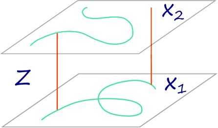
Figure 1: The $\mathbb{C}^{\times}_{q}$-fixed locus $X$ may be disconnected and the map $\pi_{\textsf{M2}}$ keeps those components of $\mathbb{C}^{\times}_{q}$-invariant curves that lie in $X$ and discards the $\mathbb{C}^{\times}_{q}$-orbits that are drawn vertically in the picture.

2.3.4

Consider the diagram of maps

in which $\iota$ is the inclusion of the fixed locus. Assuming an equivariant localization formula may be proven for $\widetilde{\mathscr{O}}_{\textsf{M2}}$, it would produce a sheaf $\widetilde{\mathscr{O}}_{\textsf{M2},\textup{localized}}$ on the fixed locus such that

$$\iota_{*}\widetilde{\mathscr{O}}_{\textsf{M2},\textup{localized}}=\widetilde{\mathscr{O}}_{\textsf{M2}}$$

in localized equivariant $K$-theory of $\textsf{M2}(Z)$. We denote

$$\widetilde{\mathscr{O}}_{\textsf{M2},\textup{localized}}=\iota_{*}^{-1}\,\widetilde{\mathscr{O}}_{\textsf{M2}}\,.$$

This puts us in the position to compare the push-forward of $\widetilde{\mathscr{O}}_{\textsf{M2},\textup{localized}}$ to the Chow variety of $X$ with the similar push-forward from the sheaf side.

2.3.5

There are natural $S(d)$-invariant maps

$$\Sigma_{d}:\operatorname{\mathsf{Chow}}(X)^{\times d}\to\operatorname{\mathsf{Chow}}(X)$$

given by addition of cycles

$$\left(\mathscr{C}_{1},\dots,\mathscr{C}_{d}\right)\mapsto\sum\mathscr{C}_{i}\,.$$

Given a sheaf $\mathscr{F}$ on $\operatorname{\mathsf{Chow}}(X)$, we define its symmetric algebra over $\operatorname{\mathsf{Chow}}(X)$ by

$$\mathsf{S}_{\operatorname{\mathsf{Chow}}}\,\mathscr{F}=\bigoplus_{d=0}^{\infty}\left(\Sigma_{d,*}\mathscr{F}^{\boxtimes d}\right)^{S(d)}\,.$$

2.3.6

The following is our main conjecture, in an abstract form:

Conjecture 1.

We have the following equality in $\mathsf{T}_{\textup{K\"{a}hler}}(Z)\times G_{q}$-equivariant $K$-theory of the Chow variety:

$$\mathsf{S}_{\operatorname{\mathsf{Chow}}}\,\pi_{\textsf{M2},*}\,\iota_{*}^{-1}\,\widetilde{\mathscr{O}}_{\textsf{M2}}=\pi_{\operatorname{\mathsf{PT}},*}\,\left(\widetilde{\mathscr{O}}_{\operatorname{\mathsf{PT}}}\otimes\mathbf{\Phi}\right)$$ (11)

where $\mathbf{\Phi}$ is a certain explicit combination of the universal sheaves on $\prod\operatorname{\mathsf{PT}}(X_{i})$ that describes the interaction of the components of $X$ inside $Z$, see Section 3.2.5 below.

The modified virtual structure sheaves $\widetilde{\mathscr{O}}_{\textsf{M2}}$ and $\widetilde{\mathscr{O}}_{\operatorname{\mathsf{PT}}}$ are discussed in Sections 3 and 4, respectively. The interaction term $\mathbf{\Phi}$ has an explicit dependence on variables $Q^{[C_{i}]}\in\operatorname{Rep}\mathsf{T}_{\textup{K\"{a}hler}}(Z)$ where $C_{i}$ is a $\mathbb{C}^{\times}_{q}$-invariant curve discarded by the map $\pi_{\textsf{M2}}$.

2.3.7

There are numerous advantages to formulating our conjectures are a comparison of sheaves on the Chow variety.

Most importantly, in this paper we make only partial progress towards constructing the sheaf $\widetilde{\mathscr{O}}_{\textsf{M2}}$. However, there is a good understanding of it over a large open set in the Chow variety and the corresponding statement (11) is highly nontrivial and may be subjected to many checks.

Further, the construction of the modified virtual structure sheaves $\widetilde{\mathscr{O}}_{\textsf{M2}}$ and $\widetilde{\mathscr{O}}_{\operatorname{\mathsf{PT}}}$ requires finding square roots of certain line bundles. For these square roots to exist globally, one may need to introduce an additional twist by a line bundle pulled back from the Chow variety, see Section 6.2.2. The formulation (11) avoids these complications modulo a certain technical provision.

2.4 Fields of 11-dimensional supergravity and degree zero DT counts

2.4.1

M-theory is a quantum theory of gravity which is believed to reduce, at low energies, to the eleven dimensional supergravity.

In this paper, we mostly focus on the contribution of membranes to the M-theory index. There is also a contribution of supergravity fields to the index which, in principle, is easier to determine because of its local nature. A conjectural connection between the field index and degree zero K-theoretic Donaldson-Thomas invariants was discovered in [25, 26]. Since this paper is a natural development of the ideas of [25], we summarize them briefly.

2.4.2

We consider M-theory on a manifold of the form (4) in the Hamiltonian formulation and linearized around a certain vacuum configuration. This means that as our configuration space we take

$$\operatorname{\mathsf{Conf}}=\frac{\{\textup{global sections of bosonic fields on $Z$}\}}{\textup{gauge equivalence}\sim}\,,$$

where the linearized bosonic fields of the eleven dimensional supergravity are a small perturbations

$${\delta}g\in\Gamma(S^{2}T^{*}Z)\,,$$

of some background metric $g_{0}$ and the $3$-form

$$A\in\Gamma(\Omega^{3}Z)\,.$$

At the linearized level, the gauge equivalence classes are the cosets by the image of the vectors fields and 2-forms on $Z$ that act by infinitesimal diffeomorphisms and

$$A\mapsto A+d\omega\,,\quad\omega\in\Gamma(\Omega^{2}Z)\,,$$

respectively. In particular, $\operatorname{\mathsf{Conf}}$ is an infinite-dimensional linear space (even for compact $Z$, since neither sections nor bundles are holomorphic at this point). In addition one imposes, in canonical gravity, the invariance under the diffeomorphisms of the eleven-dimensional space-time manifold. After the Diff$(Z)$ invariance is imposed, there is one more constraint, the so-called Hamiltonian constraint, which is a second order differential-variational equation to be obeyed by the allowed sections of the appropriate line bundle over $\operatorname{\mathsf{Conf}}$. Instead of trying to solve this constraint, for the purposes of enumerating the solutions, it is sufficient to restrict the class of metric perturbations. A convenient choice is to impose the traceless constraint on ${\delta}g$:

$${\operatorname{tr}}g_{0}^{-1}{\delta}g=0$$

where we used the background metric $g_{0}$ to make an operator $g_{0}^{-1}{\delta}g:TZ\mapsto TZ$.

The isometries of $g_{0}$ act on $\operatorname{\mathsf{Conf}}$ by linear operators.

2.4.3

While questions of regularity of sections, boundary conditions etc. are of paramount physical importance, index computations are typically less sensitive to such issues and in the present discussion they will be ignored entirely. Our computations will be formally modeled on the following basic example.

Suppose $\operatorname{\mathsf{Conf}}$ is a finite-dimensional real vector space with a linear action of a compact group $G$. In particular, $\operatorname{\mathsf{Conf}}\cong\operatorname{\mathsf{Conf}}^{*}$ as a $G$-module. Let $\mu$ be a $G$-invariant measure on $\operatorname{\mathsf{Conf}}$, which always exists. We can find a growing $G$-invariant function $f(x)$ such that the map

$${\mathsf{S}}^{\raisebox{1.42262pt}{$\scriptscriptstyle\bullet$}}\operatorname{\mathsf{Conf}}\otimes_{\mathbb{R}}\mathbb{C}\owns p(x)\mapsto p(x)e^{-f(x)}\in L^{2}(\operatorname{\mathsf{Conf}},\mu)$$ (12)

has a dense image. Neither side of (12) has a well-defined $G$-character because of infinite multiplicities, but the degree grading on polynomials allows to form the following series

$$\sum_{k\geq 0}t^{k}\,\operatorname{tr}_{\mathsf{S}^{k}\operatorname{\mathsf{Conf}}}g=\exp\left(\sum_{n\geq 1}\frac{t^{n}}{n}\,\operatorname{tr}_{\operatorname{\mathsf{Conf}}}g^{n}\right)\,,\quad g\in G\,,$$

which will replace for us the $G$-character of $L^{2}(\operatorname{\mathsf{Conf}},\mu)$.

2.4.4

The odd degrees of freedom are

$$\Psi\oplus\Psi^{*}=\{\textup{global sections of fermionic fields on $Z$}\}\Big{/}\sim\,,$$ (13)

where fermionic fields of M-theory are the Rarita-Schwinger fields $\psi_{\pm}$ of spin 3/2. They transform in the representations

$$V^{3/2}_{\pm}=\operatorname{Ker}\left(V\otimes S_{\pm}\to S_{\mp}\right)$$

of the group $Spin(V)$ where

$$V=T_{z_{0}}Z\cong\mathbb{R}^{10}\,,$$

and $S_{\pm}$ are the spinor representations of $Spin(V)$, the universal cover of $SO(V)$. The Lie algebra of the gauge transformations is also extended to include the transformations

$$\psi\mapsto\psi+\nabla\textup{spinor}\,,$$

that change $\psi$ by a derivative of a spinor field. If we linearize around the vanishing RS fields then the configuration superspace is a direct product of its even and odd subspaces.

2.4.5

Building the space $L^{2}(\operatorname{\mathsf{Conf}},{\Lambda}^{\!\raisebox{1.42262pt}{$\scriptscriptstyle\bullet$}\,}\Psi^{*})$ requires a choice of the polarization in (13). An important point, which will be revisited below, is that the two natural choices

$$\Psi^{*}=\{\textup{global $\psi_{\pm}$ on $Z$}\}$$

give dual and inequivalent answers. For now, we fix one choice, namely $\psi_{+}$. Then the $\operatorname{Iso}(g_{0})$-index of $L^{2}(\operatorname{\mathsf{Conf}},{\Lambda}^{\!\raisebox{1.42262pt}{$\scriptscriptstyle\bullet$}\,}\Psi^{*})$ is the symmetric algebra of global sections of the following virtual bundle

$$\underline{\mathit{Conf}_{\textup{super}}}= S^{2}TZ-1$$ traceless metric (14)

$$-TZ$$ modulo diffeomorphisms

$$\Omega^{3}Z-\Omega^{2}Z+\Omega^{1}Z-1$$ 3-form modulo exact

$$-TZ\otimes S_{+}+S_{+}+S_{-} \textup{RS field modulo exact}\,.$$

2.4.6

Now suppose that $g_{0}$ is a Kähler metric and choose $G\subset\operatorname{Iso}(g_{0})$ so that it acts trivially on the trivial bundle $\Omega^{5,0}Z$. Then

$$S_{\pm}=\Lambda^{\textup{even/odd}}T^{1,0}Z$$

as $G$-bundles. A direct computation with characters proves the following key

Proposition 2.1 ([25]).

For $G$ as above, we have

$$\underline{\mathit{Conf}_{\textup{super}}}=-T^{1,0}\otimes(S_{+}-S_{-})$$

as $G$-bundles and so, by Dolbeault,

$$L^{2}(\operatorname{\mathsf{Conf}},{\Lambda}^{\!\raisebox{1.42262pt}{$\scriptscriptstyle\bullet$}\,}\Psi^{*})={\Lambda}^{\!\raisebox{1.42262pt}{$\scriptscriptstyle\bullet$}\,}\chi(TZ)\,,$$

as virtual $G$-modules, where $\chi$ is the holomorphic Euler characteristic.

Note that changing the roles of $S_{+}$ and $S_{-}$ changes the answer to

$$\overline{{\Lambda}^{\!\raisebox{1.42262pt}{$\scriptscriptstyle\bullet$}\,}\chi(TZ)}={\mathsf{S}}^{\raisebox{1.42262pt}{$\scriptscriptstyle\bullet$}}\chi(T^{*}Z)\,.$$

The conjectural formula of [25] for degree 0 DT invariants is, suitably interpreted, the product of both answers, that is ${\mathsf{S}}^{\raisebox{1.42262pt}{$\scriptscriptstyle\bullet$}}\chi(T^{*}Z-TZ)$, see Conjecture 2 below.

It would be interesting to have a good explanation of this doubling phenomenon, which may be compared to the squaring that happens in the degree 0 part of the correspondence between cohomological Gromov-Witten and Donaldson-Thomas invariants of 3-folds [24]. We don’t discuss it further in the present paper and refer the reader to the original paper [25] for more information.

2.4.7

Suppose $Z$ is the total space of two line bundles $\mathscr{L}_{1}$ and $\mathscr{L}_{2}$ over a 3-fold $X$, such that $\mathscr{L}_{1}\otimes\mathscr{L}_{2}=\mathscr{K}_{X}$. Then, by localization,

$$\chi(Z,TZ)=\chi\left(X,\frac{TZ\big{|}_{X}}{(1-\mathscr{L}_{1}^{-1})(1-\mathscr{L}_{2}^{-1})}\right)$$

and further

$$\frac{T^{*}Z\big{|}_{X}-TZ\big{|}_{X}}{(1-\mathscr{L}_{1}^{-1})(1-\mathscr{L}_{2}^{-1})}=\mathscr{K}_{X}-\mathscr{O}_{X}+\\ \frac{\mathscr{L}_{1}}{(1-\mathscr{L}_{1})(1-\mathscr{L}_{2}^{-1})}\left(TX+\mathscr{K}_{X}-T^{*}X-\mathscr{K}_{X}^{*}\right)\,.$$ (15)

Now note that if $\mathbb{C}^{\times}_{q}$ acts on $\mathscr{L}_{1}$ and $\mathscr{L}_{2}$ with weights $q$ and $q^{-1}$ respectively, then all weights occurring in the second line of (15) are positive, and therefore the symmetric algebra of that term is well-defined in $\mathbb{C}^{\times}_{q}$-equivariant K-theory. Discounting the contribution of the first term in the RHS of (15) as a (possibly infinite) prefactor, we make contact with the following reformulation of a conjecture from [25].

2.4.8

Let

$$\operatorname{Hilb}(X,\textup{points})=\bigsqcup_{n\geq 0}\operatorname{Hilb}(X,n)$$

be the Hilbert scheme of points of $X$ and consider the following sheaf on it

$$\widetilde{\mathscr{O}}_{\textup{vir}}=(-q)^{\chi(\mathscr{O}/\mathscr{I})}\,\mathscr{O}_{\textup{vir}}\otimes\left(\mathscr{K}_{\textup{vir}}\otimes\det H^{0}(\mathscr{O}/\mathscr{I}\otimes(\mathscr{L}_{1}-\mathscr{L}_{2}))\right)^{1/2}$$

where the $\mathscr{O}/\mathscr{I}$ is the structure sheaf of the universal $0$-dimensional subscheme of $X$. This is special case of the sheaf $\widetilde{\mathscr{O}}_{\textup{vir}}$ defined and discussed below, so we don’t go into a further discussion of it here.

Conjecture 2 ([25]).

For $X$ as above

$$\chi\left(\operatorname{Hilb}(X,\textup{points}),\widetilde{\mathscr{O}}_{\textup{vir}}\right)={\mathsf{S}}^{\raisebox{1.42262pt}{$\scriptscriptstyle\bullet$}}\chi\left(X,\frac{q\mathscr{L}_{1}\left(TX+\mathscr{K}_{X}-T^{*}X-\mathscr{K}_{X}^{*}\right)}{(1-q\mathscr{L}_{1})(1-q\mathscr{L}_{2}^{-1})}\right)$$

We expect that the conjectural PT/DT correspondence [30] extends to K-theoretic invariants as follows

$$\chi\left(\operatorname{\mathsf{PT}}(X),\widetilde{\mathscr{O}}_{\textup{vir}}\right)\overset{?}{=}\frac{\chi\left(\operatorname{Hilb}(X,\textup{curves}),\widetilde{\mathscr{O}}_{\textup{vir}}\right)}{\chi\left(\operatorname{Hilb}(X,\textup{points}),\widetilde{\mathscr{O}}_{\textup{vir}}\right)}\,.$$ (16)

2.4.9

To get a sense what this means in concrete terms, take $Z=\mathbb{C}^{5}$ and let $t_{1},\dots,t_{5}$ be the weights of the coordinate directions. They satisfy

$$\prod t_{i}=1\,.$$ (17)

We have

$$\chi(Z,TZ^{*})=\frac{\sum_{1}^{5}t_{i}^{-1}}{\prod_{1}^{5}(1-t_{i}^{-1})}\,,$$

where the denominator may be symmetrized using (17). Identity (15) says that

$$\frac{\sum_{1}^{5}t_{i}^{-1}-\sum_{1}^{5}t_{i}}{\prod_{1}^{5}(t_{i}^{1/2}-t_{i}^{-1/2})}=\\ \frac{-(t_{1}t_{2}t_{3})^{1/2}+(t_{1}t_{2}t_{3})^{-1/2}}{\prod_{1}^{3}(t_{i}^{1/2}-t_{i}^{-1/2})}\,+\frac{\prod_{i<j\leq 3}\left((t_{i}t_{j})^{1/2}-(t_{i}t_{j})^{-1/2}\right)}{\prod_{1}^{5}(t_{i}^{1/2}-t_{i}^{-1/2})}$$ (18)

whenever (17) is satisfied.

The first term in the left-hand side of (18) does not involve $t_{4}$ or $t_{5}$ and may be viewed as a perturbative contribution to the integrals over the Hilbert schemes. The second term in the left-hand side of (18), which we will denote $F(t)$, and in which one can already recognize the contribution of the Hilbert scheme of 1 point, computes the degree zero DT invariants as follows.

The bundles $\mathscr{L}_{1}$ and $\mathscr{L}_{2}$ are trivial bundles with weights $t_{4}$ and $t_{5}$, respectively. Hence on the Hilbert scheme $\operatorname{Hilb}(\mathbb{C}^{3},n)$ of $n$ points the line bundle $\det H^{0}(\mathscr{O}/\mathscr{I}\otimes(\mathscr{L}_{1}-\mathscr{L}_{2}))$ is trivial with weight $(t_{4}/t_{5})^{n}=q^{2n}$. Therefore, Conjecture 2 means

$$\sum_{n\geq 0}(-q)^{n}\chi\left(\operatorname{Hilb}(\mathbb{C}^{3},n),\mathscr{O}_{\textup{vir}}\otimes\mathscr{K}_{\textup{vir}}^{1/2}\right)\overset{?}{=}\exp\left(\sum_{n=1}^{\infty}\frac{F(t^{n})}{n}\right)$$

with

$$t_{4}=q^{1/2}(t_{1}t_{2}t_{3})^{-1/2}\,,\quad t_{5}=q^{-1/2}(t_{1}t_{2}t_{3})^{-1/2}\,.$$

The fact that the right-hand side of (18) has a full 5-dimensional symmetry is a very nontrivial confirmation of the M-theory paradigm.

3 The DT integrand

3.1 The modified virtual structure sheaf

3.1.1

The DT moduli spaces of $X$, in their original definition [34], parameterize ideal sheaves $\mathscr{I}\subset\mathscr{O}_{X}$ of $1$-dimensional subschemes in $X$. They have a perfect obstruction theory described by

$$\operatorname{Def}-\operatorname{Obs} =\chi(\mathscr{O}_{X})-\chi(\mathscr{I},\mathscr{I})$$ (19)

$$=\chi(\mathscr{F})+\chi(\mathscr{F},\mathscr{O}_{X})-\chi(\mathscr{F},\mathscr{F})\,,$$

where $\mathscr{F}=\mathscr{O}/\mathscr{I}$ is the universal $1$-dimensional sheaf on $X$.

Other stability conditions for complexes of sheaves on $X$ lead to alternative DT moduli spaces. In particular, in the Pandharipande-Thomas chamber [30], the moduli spaces parameterize pairs

$$s:\mathscr{O}_{X}\to\mathscr{F}$$

where $\mathscr{F}$ is a pure $1$-dimensional sheaf and the cokernel of the section $s$ has finite length. The formula for the $K$-theory class of their obstruction theory is the same.

3.1.2

A perfect obstruction theory defines, in the usual way (see for example [12]), a virtual structure sheaf $\mathscr{O}_{\textup{vir}}$. If, for instance, $p\in\operatorname{\mathsf{PT}}(X)$ is an isolated fixed point of a torus $\mathsf{T}$ and

$$\operatorname{Def}_{p}-\operatorname{Obs}_{p}=\sum a_{i}-\sum b_{i}\,,\quad a_{i},b_{j}\in\mathsf{T}^{\vee}\,,$$

is the character of the deformation theory at $p$ then the localization of $\mathscr{O}_{\textup{vir}}$ at $p$ in $\mathsf{T}$-equivariant $K$-theory equals

$$\mathscr{O}_{\textup{vir},\textup{localized}}=\frac{\prod\left(1-b_{i}^{-1}\right)}{\prod\left(1-a_{i}^{-1}\right)}\,.$$ (20)

3.1.3

The virtual canonical bundle is defined by

$$\mathscr{K}_{\textup{vir}}=\frac{\det\operatorname{Obs}}{\det\operatorname{Def}}\,.$$

Of particular importance to us will be its square root $\mathscr{K}_{\textup{vir}}^{1/2}$, compare with Section 2.2.6.

Different choice of the square roots (related by the $2$-torsion in the Picard group) correspond to different boundary conditions for fermions in the theory. This means they define different sectors of the theory that have to be matched in concrete computations.

If $p$ is an isolated fixed point as in (20) then

$$\left(\mathscr{O}_{\textup{vir}}\otimes\mathscr{K}_{\textup{vir}}^{1/2}\right)_{\textup{localized}}=\frac{\prod\left(b_{i}^{1/2}-b_{i}^{-1/2}\right)}{\prod\left(a_{i}^{1/2}-a_{i}^{-1/2}\right)}\,.$$ (21)

3.1.4

The twist by $\mathscr{K}_{\textup{vir}}^{1/2}$ brings K-theoretic DT computations much closer to familiar sheaf cohomology problems.

There is a certain degree of duality between deformations and obstructions in DT theory, with perfect duality in the case when $\mathscr{K}_{X}$ restricts to the trivial bundle on the support of $\mathscr{F}$. It is, therefore, useful to keep in mind the following baby example of a self-dual obstruction theory, which we will revisit below.

Let $M$ be a smooth algebraic variety, viewed as zero section

$$s:M\to T^{*}M$$

of its cotangent bundle. The corresponding obstruction theory is

$$\operatorname{Def}-\operatorname{Obs}=TM-T^{*}M$$

with

$$\mathscr{O}_{\textup{vir}}=s^{*}(\mathscr{O}_{M})=\sum_{k=0}^{\dim M}(-1)^{k}\Lambda^{k}TM\,.$$

We have

$$\mathscr{K}_{\textup{vir}}^{1/2}=\mathscr{K}_{M}$$

and hence

$$\mathscr{O}_{\textup{vir}}\otimes\mathscr{K}_{\textup{vir}}^{1/2}=(-1)^{\dim M}\sum_{k=0}^{\dim M}(-1)^{k}\,\Omega^{k}M\,.$$ (22)

If a torus scales the fibers of $T^{*}M$ with weight $t$ then it scales the $\Omega^{k}M$ term in (22) with weight $t^{k-\dim M/2}$. Thus

$$\chi\left(\mathscr{O}_{\textup{vir}}\otimes\mathscr{K}_{\textup{vir}}^{1/2}\right)=\sum_{p,q}(-1)^{p-\dim/2}(-t)^{q-\dim/2}H^{p}(\Omega^{q}M)$$

is a specialization of the centered Hodge polynomial of $M$.

3.1.5

A sheaf $\mathscr{G}$ on $X$ gives a line bundle

$$\mathbb{L}_{\mathscr{G}}=\det H^{*}(X,\mathscr{F}\otimes\mathscr{G})$$

on the DT moduli spaces, where $\mathscr{F}$ is the universal $1$-dimensional sheaf, e.g. $\mathscr{F}=\mathscr{O}/\mathscr{I}$ in the Hilbert scheme chamber.

3.1.6

If $\mathscr{G}$ is $1$-dimensional, then the degree of $\mathbb{L}_{\mathscr{G}}$ may be computed as follows. Let $B$ be $1$-dimensional family of sheaves and let $\mathscr{F}$ denote the corresponding sheaf on $B\times X$. Let

$$p_{X}:B\times X\to X$$

denote the projection and let

$$\operatorname{\mathsf{sweep}}(B)=p_{X}\left(\operatorname{\mathsf{cycle}}(\mathscr{F})\right)$$

denote the 2-cycle in $X$ swept by the cycles of sheaves in $B$. From Grothendieck-Riemann-Roch, we have

$$\deg_{B}\mathbb{L}_{\mathscr{G}}=\operatorname{\mathsf{sweep}}(B)\,\cdot\,\operatorname{\mathsf{cycle}}(\mathscr{G})\,.$$ (23)

Note that families with trivial sweep are precisely those contracted by the map to the Chow variety and, in fact, it can be shown [19] that the bundle $\mathbb{L}_{\mathscr{G}}$ is pulled back from the Chow variety.

3.1.7

Symmetrically, for 1-dimensional $\mathscr{G}$, the bundle $\mathbb{L}_{\mathscr{G}}\in\operatorname{Pic}\operatorname{\mathsf{DT}}(X)$ depends only on $\operatorname{\mathsf{cycle}}(\mathscr{G})$ and, in fact, only on its rational equivalence class.

3.1.8

We now have prepared all ingredients for the definition of the modified virtual structure sheaf $\widetilde{\mathscr{O}}_{\operatorname{\mathsf{DT}}}$.

Let $X$ be the fixed locus of $\mathbb{C}^{\times}_{q}$-action on a nonsingular Calabi-Yau 5-fold $Z$ as above. Since $\mathbb{C}^{\times}_{q}$ preserves the holomorphic 5-form $\Omega^{5}$, we have

$$N_{X}Z=\mathscr{L}_{1}\oplus\mathscr{L}_{2}$$

where $\mathbb{C}^{\times}_{q}$ acts with weights $q$ and $q^{-1}$, respectively. The triviality of $\mathscr{K}_{Z}$ implies

$$\mathscr{L}_{1}\otimes\mathscr{L}_{2}=\mathscr{K}_{X}\,.$$

The roles of line bundles $\mathscr{L}_{1}$ and $\mathscr{L}_{2}$ will not be symmetric, reflecting the choice stressed in Section 2.1.4: the $\mathscr{L}_{1}$ direction is attracting as $q\to 0$, while the $\mathscr{L}_{2}$ direction is repelling.

Given a $1$-dimensional sheaf $\mathscr{F}$ on $X$, we denote by

$$\chi=\chi(\mathscr{F})\,,\quad\beta=\left[\operatorname{\mathsf{cycle}}(\mathscr{F})\right]\in H_{2}(X,\mathbb{Z})$$

its discrete invariants. The virtual dimension of DT moduli spaces at a point corresponding to $\mathscr{F}$ equals

$$\textup{vir dim}=-(\mathscr{K}_{X},\beta)=-(\mathscr{L}_{1}+\mathscr{L}_{2},\beta)\,.$$

Definition 1.

We define

$$\widetilde{\mathscr{O}}_{\operatorname{\mathsf{DT}}}=\textup{prefactor}\,\,\mathscr{O}_{\textup{vir}}\otimes\left(\mathscr{K}_{\textup{vir}}\otimes\mathbb{L}_{\mathscr{L}_{1}-\mathscr{L}_{2}}\right)^{1/2}$$ (24)

where

prefactor $$=(-1)^{\frac{(\mathscr{L}_{1}-\mathscr{L}_{2},\beta)}{2}}\,(-q)^{-\frac{\textup{vir dim}}{2}+\chi}\,Q^{\beta}$$ (25)

$$=(-1)^{(\mathscr{L}_{1},\beta)+\chi}\,q^{-\frac{\textup{vir dim}}{2}+\chi}\,Q^{\beta}\,.$$

Note that in the $\mathbb{L}_{\mathscr{L}_{1}-\mathscr{L}_{2}}$ term we have the difference of $K$-classes and not the ratio $\mathscr{L}_{1}\otimes\mathscr{L}_{2}^{-1}\in\operatorname{Pic}(X)$. There is a simple explanation for the this form of the DT integrand, see Section 5.1.5.

We will see in Section 6.2.2 that

$$\mathscr{K}_{\textup{vir}}\otimes\mathbb{L}_{\mathscr{L}_{1}-\mathscr{L}_{2}}=\textup{square}\otimes\mathbb{L}_{c_{1}(\mathscr{L}_{1})\cap c_{1}(\mathscr{L}_{2})}\,,$$

where the second factor is pulled back from the Chow variety of $X$, as in the preceding discussion.

3.2 The interaction term $\mathbf{\Phi}$

3.2.1 $A_{r-1}$ surface fibrations

For the discussion of the interaction between different components of $Z^{\mathbb{C}^{\times}_{q}}$ it is convenient to keep in mind the following simplest example. Let

$$Z_{1}=\begin{matrix}\mathscr{L}_{1}\oplus\mathscr{L}_{2}\\ \downarrow\\ X\end{matrix}\,,\quad\mathscr{L}_{1}\otimes\mathscr{L}_{2}=\mathscr{K}_{X}\,,$$

be the total space of two line bundles over $X$. Let $\mathbb{C}^{\times}_{q}$ scale the fibers by $\textup{diag}(q,q^{-1})$ and let $\mu_{r}\subset\mathbb{C}^{\times}_{q}$ be the group of $r$th roots of unity. Let

be the minimal resolution of the quotient $Z_{1}\big{/}\mu_{r}$. It fibers over $X$ in $A_{r-1}$-surfaces

$$A_{r-1}=\widetilde{\mathbb{C}^{2}/\mu_{r}}\,,$$

that is, minimal resolutions of the the singularity $x^{r}=yz$. The quotient in

$$1\to\mu_{r}\to\mathbb{C}^{\times}_{q}\xrightarrow{\,\,\,q\mapsto q^{r}\,}\mathbb{C}^{\times}_{q^{r}}\to 1$$

acts canonically on $Z_{r}$ and

$$Z_{r}^{\mathbb{C}^{\times}_{q^{r}}}=X\times\{\textup{$r$ points}\}\,.$$

In this example, we will see the rank $r$ Donaldson-Thomas theory on $X$ appear from the interaction of rank $1$ theories on $r$ copies of $X$, see Section 5.5.

3.2.2 Unbroken curves

Going back to the general situation, let $C\subset Z$ be a reduced connected $\mathbb{C}^{\times}_{q}$-invariant curve. We say that $C$ is unbroken if $\mathbb{C}^{\times}_{q}$ acts nontrivially on each component of $C$. This implies $C$ is rational, at worst nodal, and that the two branches at each node have opposite weights. It also implies it has two nonsingular fixed points $p_{1},p_{2}\in C$ which lie on two different components $X_{1}$ and $X_{2}$ of the fixed locus. We say that $C$ flows from $X_{2}$ to $X_{1}$ if the $\mathbb{C}^{\times}_{q}$-weight of $T_{p_{1}}C$ is positive. We denote by $\mathscr{U}_{21}$ the moduli space of unbroken curves from $X_{2}$ to $X_{1}$.

Since both spaces $T_{p_{i}}Z$ have three trivial $\mathbb{C}^{\times}_{q}$-weights, there are two possibilities for the normal bundle to $C$, namely

$$N_{C}Z=\begin{cases}\mathscr{O}(-p_{1}-p_{2})\oplus\mathscr{O}^{\oplus 3}\,,&\textup{or}\\ \mathscr{O}(-p_{1})\oplus\mathscr{O}(-p_{2})\oplus\mathscr{O}^{\oplus 2}\,,\end{cases}$$ (26)

as $\mathbb{C}^{\times}_{q}$-equivariant sheaves. In the first case in (26),

$$\mathscr{U}_{21}\cong X_{1}\cong X_{2}$$

with the obstruction bundle

$$H^{1}(C,\mathscr{O}(-p_{1}-p_{2}))\cong\mathscr{L}_{1}\big{|}_{p_{i}}\otimes\mathscr{L}_{2}\big{|}_{p_{i}}\cong\mathscr{K}_{X_{i}}\big{|}_{p_{i}}\quad i=1,2\,,$$

where, as usual, we denote by $\mathscr{L}_{1}$ and $\mathscr{L}_{2}$ the $\mathbb{C}^{\times}_{q}$-eigenbundles in the normal bundle to the fixed locus. In the second case in (26), the deformations are $2$-dimensional and unobstructed. The moduli space of unbroken curves embeds

$$X_{2}\hookleftarrow\mathscr{U}_{21}\hookrightarrow X_{1}$$

in each of the $X_{i}$ as a smooth surface.

3.2.3 Threefold and surface interactions

We will refer to the two cases in (26) as the threefold and surface interactions, respectively. For example, there is a threefold interaction between any pair of fixed components in the example of Section 3.2.1. The corresponding unbroken curves are the $(-2)$-curves in the $A_{r-1}$-fibers.

An example of a surface interaction may be constructed as follows. Take

$$Y=\begin{matrix}\mathscr{O}(-1)\oplus\mathscr{O}(-1)\\ \downarrow\\ \mathbb{P}^{1}\end{matrix}$$

and make $\mathbb{C}^{\times}_{q}$ act on $Y$ by scaling the base $\mathbb{P}^{1}$ and so that there is a trivial weight in the fiber over each fixed point. Instead of $Y$ we could have taken many other toric CY threefold that contain the $\mathbb{C}^{\times}_{q}$-invariant curve with an $\mathscr{O}(-1)\oplus\mathscr{O}(-1)$ normal bundle. Consider a $Y$-bundle over a surface $S$ associated to a principal $(\mathbb{C}^{\times})^{3}$-bundle $P$

$$Z=P\times_{(\mathbb{C}^{\times})^{3}}Y\,,\quad c_{1}(P)=\mathscr{K}_{S}$$

We see that $\mathscr{K}_{Z}\cong\mathscr{O}_{Z}$, $X_{1}$ and $X_{2}$ are line bundles over $S$, and

$$\mathscr{U}_{21}\cong S$$

is embedded in each of them as the zero section. Since the surface $S$ is arbitrary, we conclude $\mathscr{K}_{\mathscr{U}_{21}}$ may not be a square.

3.2.4 The operators $\Phi_{ij}$

The obstruction theory

$$\operatorname{Def}-\operatorname{Obs}=H^{*}(C,N_{C}Z)$$

gives $\mathscr{U}_{21}$ a virtual structure sheaf of virtual dimension $2$. For 3-fold interactions, the corresponding virtual canonical bundle is always a square with

$$\widetilde{\mathscr{O}}_{\mathscr{U}_{21}}=\mathscr{K}_{X_{i}}-\mathscr{O}_{X_{i}}\,.$$

For surface interactions, we assume that the square root in

$$\widetilde{\mathscr{O}}_{\mathscr{U}_{21}}=\mathscr{K}^{1/2}_{\mathscr{U}_{21}}$$

exists and we define, in either case,

$$\Phi_{21}=\operatorname{eval}_{*}\widetilde{\mathscr{O}}_{\mathscr{U}_{21}}\,,$$

where

$$\operatorname{eval}:\mathscr{U}_{21}\to X_{2}\times X_{1}$$

sends an unbroken curve $C$ to the fixed points $(p_{2},p_{1})$. We will denote by the same symbol $\Phi_{21}$ the corresponding Fourier-Mukai operator

$$\mathscr{F}_{1}\xrightarrow{\,\,\Phi_{21}\,\,}p_{X_{2},*}\left(\Phi_{21}\otimes p_{X_{1}}^{*}\,\mathscr{F}_{1}\right)\,.$$

For example, for 3-fold interactions

$$\Phi_{21}\,\mathscr{F}_{1}=\mathscr{K}_{X}\otimes\mathscr{F}_{1}-\mathscr{F}_{1}\,.$$

3.2.5 The interaction

Let $X_{1}$ and $X_{2}$ be two components of $X$ as above and let $\mathscr{F}_{1}$ and $\mathscr{F}_{2}$ denote the universal $1$-dimensional sheaves over the DT moduli spaces for $X_{1}$ and $X_{2}$. Using the operator $\Phi_{21}$, we can define the following $K$-theory class

$$\mathscr{X}_{21}=\chi(\mathscr{O}_{X_{2}}-\mathscr{F}_{2},\Phi_{21}(\mathscr{O}_{X_{1}}-\mathscr{F}_{1}))$$ (27)

which may be compared to the formula (19) for the virtual tangent space to DT moduli spaces.

We define

$$\mathbf{\Phi}=\bigotimes_{i<j}\mathsf{S}\,Q^{[C_{ij}]}\,\mathscr{X}_{ji}\,,$$ (28)

where $S$ denotes the symmetric algebra,

$$[C_{ij}]\in H_{2}(Z,\mathbb{Z})$$

is the class of the unbroken curve flowing from $X_{j}$ to $X_{i}$, and the indexing is the components is such that curves flow from larger components to smaller ones.

3.2.6 An example

For 3-fold interactions, we have, using Serre duality

$$\mathscr{X}_{21}=-\chi(\mathscr{I}_{2},\mathscr{I}_{1})-\overline{\chi(\mathscr{I}_{1},\mathscr{I}_{2})}\\$$ (29)

where $[\mathscr{I}]=[\mathscr{O}_{X}]-[\mathscr{F}]$ and bar denotes dual. Such interaction terms occur naturally in higher rank DT theory, see Section 5.4 below.

3.2.7 Perturbative contributions

Note that the Euler characteristic (27) may not be well-defined if $X_{i}$’s are not proper. However, the difference

$$\mathscr{X}^{\prime}_{21}=\mathscr{X}_{21}-\chi(\mathscr{O}_{X_{2}},\Phi_{21}\mathscr{O}_{X_{1}})=\\ -\chi(\mathscr{F}_{2},\Phi_{21}\mathscr{O}_{X_{1}})-\chi(\mathscr{O}_{X_{2}},\Phi_{21}\mathscr{F}_{1})+\chi(\mathscr{F}_{2},\Phi_{21}\mathscr{F}_{1})$$ (30)

is well-defined and differs from (27) only by a constant, even if infinite-dimensional, vector space $\chi(\mathscr{O}_{X_{2}},\Phi_{21}\mathscr{O}_{X_{1}})$. The character of its symmetric algebra

$$\mathsf{S}\,Q^{[C_{12}]}\,\chi(\mathscr{O}_{X_{2}},\Phi_{21}\mathscr{O}_{X_{1}})$$

may be regularized using any of the traditional approaches. From the point of view of DT theory on X, it comes out as an overall prefactor, also known as a perturbative contribution.

4 The index of membranes

4.1 Membrane moduli

4.1.1 Multiple curves

Recall that the moduli space $\textsf{M2}(Z)$ of stable membranes in $Z$ is supposed to be a certain compactification of the moduli space of immersed holomorphic curves $C\subset Z$. One such compactification is the moduli space of stable maps; compactifications using moduli of sheaves on $Z$ may also be considered. While it is entirely possible that the M2-brane contributions to the M-theory indexed may be calculated using such moduli spaces, in this paper we pursue an alternative route.

The main geometric difficulty in dealing with holomorphic curves is degeneration to multiple curves, e.g. the ellipse

$$y^{2}=\lambda(1-x^{2})$$

degenerating to the double line $y^{2}=0$ as $\lambda\to 0$. A physicist may call a multiple curve a bound state of several M2-branes. In the moduli space of stable maps, the $\lambda\to 0$ limit is the double cover of the $y=0$ line branched over the points $x=\pm 1$, which remember the branchpoints of the $x$-projection of the original ellipse. In the Hilbert scheme of curves, the limit would just be the subscheme of the plane cut out by $y^{2}=0$, with no memory of the shape of the original conic.

One reason we don’t try to construct membrane moduli using sheaves on $Z$ or stable maps to $Z$ is that these don’t give natural bounded moduli spaces for given degree, recall the discussion of Section 2.2.10. For example, in the above example, there could be double covers of $y=0$ with an arbitrary large number of branchpoints or this line may be the support of a sheaf with an arbitrary large Euler characteristic.

4.1.2 Maps from schemes

In this paper, we look at maps

$$f:C\to Z$$ (31)

from $1$-dimensional schemes $C$ to $Z$. In the above example, this would be just the inclusion of the double line. In general $f$ need not be injective, like in the case of an immersion of a smooth curve $C$.

In practical terms, a map $f$ may be represented by a subscheme

$$C\subset Z\times\mathbb{P}^{N}$$

for some $N\gg 0$, with the map $f$ being the projection to the first factor. Using such presentation, one defines the normal sheaf to the map $f$ by

$$N_{f}=N_{C}\left(Z\times\mathbb{P}^{N}\right)-\mathscr{O}_{C}\otimes T\mathbb{P}^{N}\,.$$

Here

$$N_{C}\left(Z\times\mathbb{P}^{N}\right)=\operatorname{Hom}(\mathscr{I}_{C},\mathscr{O}_{C})\,,$$

where $\mathscr{I}_{C}$ is the ideal sheaf of $C$ and $\mathscr{O}_{C}$ is its structure sheaf.

When $C$ is nice, e.g. smooth or a local complete intersection, $N_{f}$ is a vector bundle of rank $4$ and degree $2g-2$. However, in general it can be much larger, reflecting the singularities of the moduli spaces of maps (31). Some strategies for dealing with large $N_{f}$ will be discussed below.

4.1.3 Stability conditions

We impose the following stability conditions on the maps (31):

1. The map $f$ is an isomorphism on its image away from a finite set of points in $C$.

2. For any proper subscheme $C^{\prime}\subset C$

   $$\frac{\chi(\mathscr{O}_{\mathbb{C}^{\prime}})}{\deg f(C^{\prime})}>\frac{\chi(\mathscr{O}_{\mathbb{C}})}{\deg f(C)}$$ (32)

   which means that $\chi(\mathscr{O}_{\mathbb{C}^{\prime}})f(C)-\chi(\mathscr{O}_{\mathbb{C}})f(C^{\prime})$ is a nonnegative and nonzero linear combination of the components of $\operatorname{supp}f(C)$.

For example, a double line $C\subset\mathbb{P}^{2}$ is stable since $\chi(\mathscr{O}_{\mathbb{C}})=1$ and $\chi(\mathscr{O}_{\mathbb{C}^{\prime}})\geq 1$ for any subscheme of $C$.

More generally, let $C$ be double zero section inside the total space of line bundle $\mathscr{L}$ over a curve $B$. Then

$$\chi(\mathscr{O}_{C})=2\chi(\mathscr{O}_{B})-\deg\mathscr{L}$$

and so (32) means

$$\textup{$C$ is stable}\,\,\Leftrightarrow\,\,\deg\mathscr{L}>0\,.$$

In other words, membranes can only stack up in positive direction of the normal bundle.

4.1.4 CM property

A $1$-dimensional scheme is Cohen-Macaulay if for every point $x\in C$ there is a function $f$ vanishing at $x$ which is not a zero-divisor.

If this condition is violated at some point $x\in C$ then

$$\mathscr{I}_{C^{\prime}}=\operatorname{Ann}\mathfrak{m}_{x}\subset\mathscr{O}_{C}\,,$$

where $\mathfrak{m}_{x}$ is the ideal of functions vanishing at $x$, is a nontrivial ideal of finite length. Thus

$$\mathscr{O}_{C^{\prime}}=\mathscr{O}_{C}/\mathscr{I}_{C^{\prime}}$$

is a proper subscheme with

$$\chi(\mathscr{O}_{C^{\prime}})<\chi(\mathscr{O}_{C})\,,\quad[f(C^{\prime})]=[f(C)]\,.$$

Therefore, the sources $C$ of all stable maps (31) are Cohen-Macaulay.

Maps from 1-dimensional Cohen-Macaulay schemes to projective varieties were studied by Hønsen in [15], who constructed their moduli space as a proper separated algebraic space for given $\deg f(C)$ and $\chi(\mathscr{O}_{C})$. He imposes the first, but not the second stability condition in Section 4.1.3.

4.1.5 Boundedness

For any map (31), the Euler characteristic $\chi(\mathscr{O}_{C})$ may be bounded below in terms of the degree of $f(C)$. Stability (32) also bounds it from above. Therefore, stable maps (31) form a bounded family once the degree of the map is fixed.

This is natural from the M-theory perspective. In M-theory there is a 3-form which couples to the worldvolume $C\times S^{1}$ of the membrane and thus keeps track of its degree. On the other hand, there are no fields that couple to the Euler characteristic of $C$ and, besides, the Euler characteristic of $C\times S^{1}$ vanishes, as it does for any smooth real 3-fold.

This means that on the membrane side of our conjectures, we sum over all Euler characteristics of membranes with no weight. The $q^{\chi}$-weight on the DT side appears only because of the $\mathbb{C}^{\times}_{q}$-action, the existence of which is an additional hypothesis on $Z$.

4.2 Deformations of membranes

4.2.1

When the normal sheaf $N_{f}$ becomes too big, the deformation theory of a map (31) becomes very complicated and technical. Perhaps some form of a virtual structure sheaf may be constructed from the normal complex of $f$. At this time, however, we are planning to pursue a more geometric approach, namely to take as $\textsf{M2}(Z)$ a certain virtual Nash blowup of the Hønsen space.

Recall that the ordinary Nash blowup of a singular space $\mathcal{M}$ remembers the limits of tangent spaces at the smooth points $\mathcal{M}_{0}\subset\mathcal{M}$ as they approach the singularities. A point of Nash blowup of $\mathcal{M}$ is described by a pair $(p,N)$, where $p\in\mathcal{M}$ and

$$N\subset T_{p}\mathcal{M}\,,\quad\dim N=\dim\mathcal{M}_{0}\,.$$

4.2.2

Our hypothetical virtual blowup $\textsf{M2}(Z)$ of the Hønsen space should parameterize maps (31) together with a subsheaf

$$N\subset N_{f}$$ (33)

of class

$$[N]=3\left[\mathscr{O}_{C}\right]+\left[\omega_{C}\right]$$

in $K$-theory of $C$, where $\omega_{C}$ is the dualizing sheaf of a Cohen-Macaulay scheme $C$. Additional conditions on $N$ form a subject of current research and will be discussed separately.

A possible physical interpretation of the extra data contained in (33) is the following. The map $f:C\to Z$ is really the bosonic part of a map of superschemes, the fermionic part of which is uniquely reconstructed in the case when $f$ is an immersion or a more general l.c.i. map. The uniqueness of the reconstruction fails when $f$ develops singularities and the subsheaf (33) stores the missing information.

4.2.3

With these additional conditions, we hope $\textsf{M2}(Z)$ to have an obstruction theory with

$$\left[\operatorname{Def}-\operatorname{Obs}\right]=\left[H^{*}(N)\right]$$

in $K$-theory of $\textsf{M2}(Z)$. We don’t expect these virtual bundles to be isomorphic, it is only their pieces with respect to a certain filtrations that should be identified.

5 Examples

5.1 Reduced local curves

5.1.1

Let $Z$ be the total space of 4 line bundles

$$Z=\begin{matrix}\mathscr{L}_{1}\oplus\mathscr{L}_{2}\oplus\mathscr{L}_{3}\oplus\mathscr{L}_{4}\\ \downarrow\\ C\end{matrix}\,,\quad\bigotimes\mathscr{L}_{i}=\mathscr{K}_{B}\,,$$

over a smooth curve $C$. As before, we make $\mathbb{C}^{\times}_{q}$ act on $\mathscr{L}_{1}$ and $\mathscr{L}_{2}$ with weights $q$ and $q^{-1}$ and hence $X$ is the total space of $\mathscr{L}_{3}\oplus\mathscr{L}_{4}$. We want to compare the DT and M-theoretic counts for the zero section $C$ inside $Z$.

5.1.2

A 3-dimensional torus $\mathsf{T}$ acts on $Z$ scaling the individual $\mathscr{L}_{i}$’s. Clearly,

$$\textsf{M2}(Z,[C])^{\mathsf{T}}=\{0\}$$

is a point representing the curve $C$ itself. We have

$$\left(\operatorname{Def}^{\textsf{M2}}-\operatorname{Obs}^{\textsf{M2}}\right)\Big{|}_{0}=H^{*}(N_{C}Z)\,,\quad N_{C}Z=\bigoplus_{i=1}^{4}\mathscr{L}_{i}\,.$$

Therefore

$$\chi\left(\textsf{M2},\widetilde{\mathscr{O}}_{\textup{vir}}\right)=\left(\det H\right)^{-1/2}{\mathsf{S}}^{\raisebox{1.42262pt}{$\scriptscriptstyle\bullet$}}H^{\vee}\,,\quad H=H^{*}(N_{C}Z)\,.$$

In practice, this means that if $\sum a_{i}-\sum b_{i}$ is the character of $H^{*}(N_{C}Z)$ then

$$\chi\left(\textsf{M2},\widetilde{\mathscr{O}}_{\textup{vir}}\right)=\prod\frac{b_{i}^{1/2}-b_{i}^{-1/2}}{a_{i}^{1/2}-a_{i}^{-1/2}}\,.$$ (34)

5.1.3

For comparison with DT theory, we need to expand (34) in powers of $q$. It is convenient to separate the $\mathbb{C}^{\times}_{q}$-moving directions

$$N_{12}=\mathscr{L}_{i}\oplus\mathscr{L}_{j}\,,\quad H_{12}=H^{*}(N_{12})\,,$$

and their contribution

$$\chi(\textsf{M2},\widetilde{\mathscr{O}}_{\textup{vir}})_{12}=\textup{contribution of $N_{12}$}$$

to (34). We compute

$$\chi(\textsf{M2},\widetilde{\mathscr{O}}_{\textup{vir}})_{12}=(-1)^{h_{1}}q^{\frac{h_{1}+h_{2}}{2}}\otimes\\ (\det H^{*}(\mathscr{L}_{1}-\mathscr{L}_{2}))^{1/2}\,\,{\mathsf{S}}^{\raisebox{1.42262pt}{$\scriptscriptstyle\bullet$}}\left(qH^{*}(\mathscr{L}_{1})\oplus qH^{*}(\mathscr{L}_{2})^{\vee}\right)\,,$$ (35)

where

$$h_{i}=\operatorname{rk}H^{*}(\mathscr{L}_{i})=\deg\mathscr{L}_{i}+1-g(C)\,.$$

In particular

$$\chi(\textsf{M2},\widetilde{\mathscr{O}}_{\textup{vir}})_{12}=(-1)^{h_{1}}q^{\frac{h_{1}+h_{2}}{2}}\,(\det H^{*}(\mathscr{L}_{1}-\mathscr{L}_{2}))^{1/2}\,(1+O(q))\,,$$ (36)

as $q\to 0$.

5.1.4

On the Donaldson-Thomas side, we have

$$\operatorname{\mathsf{PT}}(X,[C])^{\mathsf{T}}=\bigsqcup_{n\geq 0}S^{n}C\,.$$

The deformation theory of these spaces consists of deforming $C$ in the $N_{34}$-direction and a certain twisted cotangent bundle on $S^{n}C$, see below. In particular, the contribution of $H_{34}$ to PT counts is precisely $\chi(\textsf{M2},\widetilde{\mathscr{O}}_{\textup{vir}})_{34}$.

Recall that by definition (24)

$$\widetilde{\mathscr{O}}_{\operatorname{\mathsf{DT}}}=\textup{prefactor}\,\,\mathscr{O}_{\textup{vir}}\otimes\left(\mathscr{K}_{\textup{vir}}\otimes\det H^{*}(\mathscr{L}_{1}-\mathscr{L}_{2})\right)^{1/2}$$

where, dropping the constant $Q^{C}$ term,

prefactor $$=(-1)^{(\mathscr{L}_{1},\beta)+\chi}\,q^{-\frac{\textup{vir dim}}{2}+\chi}\,$$

$$=(-1)^{h_{1}+n}\,q^{\frac{h_{1}+h_{2}}{2}+n}\,$$ (37)

because $\chi(\mathscr{F})=n+1-g(C)$ for sheaves $\mathscr{F}$ parameterized by $S^{n}C$ and

$$-\textup{vir dim}=\deg\mathscr{K}_{X}=\deg\mathscr{L}_{1}+\deg\mathscr{L}_{2}\,.$$

5.1.5

The lowest term in the $q$-expansion corresponds to $n=0$. Comparing (36) to (37) we find a perfect agreement. In fact, we see that the form of the prefactor (25) is dictated by the lowest $q$-term for reduced local curves.

5.1.6

For $n>0$ there is a nontrivial obstruction bundle on $S^{n}C$. When $\mathscr{K}_{X}$ is trivial, that is, when

$$\mathscr{L}_{3}\otimes\mathscr{L}_{4}=\mathscr{K}_{C}$$

this is the cotangent bundle to $S^{n}C$ by the duality between deformations and obstructions. In general, it is a certain twisted version of $T^{*}S^{n}C$.

Let

$$\Delta\subset S^{n}C\times C$$

be the universal subscheme. Recall [4] that

$$T^{*}S^{n}C=(p_{1})_{*}\,\mathscr{O}_{\Delta}\otimes p_{2}^{*}(\mathscr{K}_{C})\,,$$ (38)

where $p_{i}$ are the projections to the two factors. More generally,

$$\operatorname{Obs}=(p_{1})_{*}\,\mathscr{O}_{\Delta}\otimes p_{2}^{*}(\mathscr{L}_{3}\otimes\mathscr{L}_{4})\,.$$

We note that the formula

$$\boxed{\chi\left({S}^{\raisebox{1.42262pt}{$\scriptscriptstyle\bullet$}}C,\widetilde{\mathscr{O}}_{\operatorname{\mathsf{DT}}}\right)=\left(\det H\right)^{-1/2}{\mathsf{S}}^{\raisebox{1.42262pt}{$\scriptscriptstyle\bullet$}}H^{\vee}\,,}\qquad H=H^{*}(\oplus\mathscr{L}_{i})\,,$$

is a generalization of a classical formula of Macdonald for the Hodge numbers of symmetric powers of a curve. Presumably, it has an elementary proof.

5.2 Double curves

5.2.1

Let $\mathscr{L}$ be a line bundle on a smooth curve $B$ and let $S_{\mathscr{L}}$ be the total space of this line bundle. If $z$ is the local coordinate along the fibers of $S_{\mathscr{L}}$ then

$$\mathbb{B}_{\mathscr{L}}=\{z^{2}=0\}\subset S_{\mathscr{L}}$$

is the infinitesimal thickening of the base $B$ in the fiber direction. We have

$$\mathscr{O}_{\mathbb{B}_{\mathscr{L}}}=\mathscr{O}_{B}\oplus\mathscr{L}^{-1}$$

as $\mathscr{O}_{B}$-module and, in particular,

$$\chi(\mathbb{B}_{\mathscr{L}})=2\chi(B)-\deg\mathscr{L}\,.$$

The normal bundle to $\mathbb{B}_{\mathscr{L}}$

$$N_{\mathbb{B}_{\mathscr{L}}}S_{\mathscr{L}}=\mathscr{L}\oplus\mathscr{L}^{2}$$

may be seen concretely as deformations of the form

$$\{z^{2}+p_{1}z+p_{2}=0\}\,,\quad p_{i}\in\Gamma(\mathscr{L}^{i})\,.$$

A very familiar example, in which there is no $H^{1}$ of the normal bundle, is the deformations of the double line to a conic in $\mathbb{P}^{2}$.

5.2.2

Let $D\subset B$ is an effective divisor of degree $d$ and let

$$s_{D}\in H^{0}(B,\mathscr{O}(D))$$

be the tautological section. It defines a map

$$F_{D}:S_{\mathscr{L}(-D)}\owns(b,z)\mapsto(b,s_{D}(b)z)\in S_{\mathscr{L}}$$

where $(b,z)$ are the base and the fiber coordinates in the domain of $F_{D}$.

The map $F_{D}$ is the blowup of $S_{\mathscr{L}}$ in the subscheme $D\subset S_{\mathscr{L}}$. Its deformations have the form

$$\operatorname{Def}(F_{D})=T_{D}\operatorname{Hilb}(S_{\mathscr{L}},d)=T_{D}\,S^{d}B+H^{0}(B,\mathscr{O}_{D}\otimes\mathscr{L})$$

and they are unobstructed. We already saw the tangent space to the symmetric power $S^{d}B$ of a curve $B$ in (38).

5.2.3

Now let $Z$ be the total space of 4 line bundles

$$Z=\begin{matrix}\mathscr{L}_{1}\oplus\mathscr{L}_{2}\oplus\mathscr{L}_{3}\oplus\mathscr{L}_{4}\\ \downarrow\\ B\end{matrix}\,,\quad\bigotimes\mathscr{L}_{i}=\mathscr{K}_{B}\,,$$

over a smooth curve $B$, and let us look for $\mathsf{T}$-invariant stable membranes in the class

$$[C]=2[B]\,.$$

Here $\mathsf{T}\cong(\mathbb{C}^{\times})^{3}$ is the torus scaling the fibers with determinant 1.

5.2.4

We will make the simplifying assumption that

$$\deg\mathscr{L}_{1}>0\geq\deg\mathscr{L}_{i}\,,\quad i=2,3,4\,,$$

in which case $C$ can only double in the direction of $\mathscr{L}_{1}$ as discussed in Section 4.1.3 and all $\mathsf{T}$-invariant stable membranes have the form

$$f_{D}:\,\,\mathbb{B}_{\mathscr{L}_{1}(-D)}\hookrightarrow S_{\mathscr{L}(-D)}\xrightarrow{\,\,\,F_{D}\,\,\,}S_{\mathscr{L}_{1}}\hookrightarrow Z\,,$$ (39)

where $D\in S^{d}B$ is an effective divisor of degree

$$0\leq d<\deg\mathscr{L}_{1}\,.$$

This range is restricted by the stability condition $\chi\left(\mathbb{B}_{\mathscr{L}_{1}(-D)}\right)<2\chi(B)$.

5.2.5

The deformation theory of the map (39) may be described as follows

$$\operatorname{Def}(f_{D})-\operatorname{Obs}(f_{D})=\operatorname{Def}(F_{D})+H^{*}\left(B,N_{\mathbb{B}_{\mathscr{L}_{1}(-D)}}S_{\mathscr{L}_{1}(-D)}+f_{D}^{*}N_{S_{\mathscr{L}_{1}}}Z\right)$$

where

$$N_{\mathbb{B}_{\mathscr{L}_{1}(-D)}}S_{\mathscr{L}_{1}(-D)} =\mathscr{L}_{1}(-D)+\mathscr{L}_{1}^{2}(-2D)\,,$$

$$f_{D}^{*}N_{S_{\mathscr{L}_{1}}}Z =(\mathscr{O}+\mathscr{L}_{1}^{-1}(D))\otimes(\mathscr{L}_{2}+\mathscr{L}_{3}+\mathscr{L}_{4})\,.$$

5.2.6

The corresponding membrane integrals are particularly easy to compute for $B=\mathbb{P}^{1}$ as then one can use the extra torus action on the base. They may be compared to the corresponding degree 2 PT integrals, which can also be computed by localization. As usual, there is, in fact, more than one PT check, as different tori may be designated as $\mathbb{C}^{\times}_{q}$.

5.3 Single interaction between smooth curves

5.3.1

Let $X_{i}$ be the components of $X=Z^{\mathbb{C}^{\times}_{q}}$ and let $C_{i}\subset X_{i}$ be a collection of smooth reduced curves, possibly empty, in each component. As in Figure 1, let $f:C\to Z$ be a $\mathbb{C}^{\times}_{q}$-invariant stable membrane such that

$$\pi_{\textsf{M2}}(f(C))\subset\sum\left[C_{i}\right]$$

where the map $\pi_{\textsf{M2}}$ of Section 2.3.3 keeps only those components that are fixed point-wise.

We denote by $C^{\prime}$ the other components of $C$ and focus here on the case when, unlike the situation depicted in Figure 1, $C^{\prime}$ is closure of a single $\mathbb{C}^{\times}_{q}$-orbit that flows from $p_{2}\in X_{2}$ to $p_{1}\in X_{1}$. The general case, when $C^{\prime}$ may be reducible or nonreduced, is expected to be covered by taking the symmetric algebra in (28).

5.3.2

There are 4 possible cases, namely

$$C=\begin{cases}C^{\prime}\,,\\ C^{\prime}\cup C_{1}\,,\\ C^{\prime}\cup C_{2}\,,\\ C^{\prime}\cup C_{1}\cup C_{2}\,,\end{cases}$$

corresponding to the 4 terms in the expansion of (27). We consider the last, most interesting case, assuming $C_{1}\neq\varnothing\neq C_{2}$. We denote by

$$\Delta N=N_{C}Z-\big{(}N_{C^{\prime}}Z+N_{C_{1}}Z+N_{C_{2}}Z\big{)}$$

the difference between the normal bundle to $Z$ and the normal bundles of its components. It may described as follows

$$\Delta N= \,T_{p_{1}}C^{\prime}\otimes T_{p_{1}}C_{1}+T_{p_{2}}C^{\prime}\otimes T_{p_{2}}C_{2}$$

$$-T_{p_{1}}Z+T_{p_{1}}C^{\prime}+T_{p_{1}}C_{1}$$

$$-T_{p_{2}}Z+T_{p_{2}}C^{\prime}+T_{p_{2}}C_{2}\,,$$ (40)

where the first line corresponds to smoothing of the two nodes, while the second line is the condition of preserving the node at $p_{1}$ if it is not smoothed.

5.3.3

The contribution of $\Delta N$ to $\widetilde{\mathscr{O}}_{\textsf{M2}}$ equals

$$\left(\det\Delta N\right)^{-1/2}{\mathsf{S}}^{\raisebox{1.42262pt}{$\scriptscriptstyle\bullet$}}\Delta N^{\vee} ={\mathsf{S}}^{\raisebox{1.42262pt}{$\scriptscriptstyle\bullet$}}\left(-N^{\vee}_{C_{1}}X_{1}\Big{|}_{p_{1}}-N_{C_{2}}X_{2}\Big{|}_{p_{2}}\right)+O(q)$$

$$=\operatorname{eval}^{*}\left(\mathscr{O}_{C_{2}}^{\vee}\boxtimes\mathscr{O}_{C_{1}}\right)+O(q)\,,$$

as $q\to 0$. We thus see that the form of the interaction described in Section 3.2.5 is dictated already by the lowest $q$-term in the simplest interacting geometry.

5.4 Higher rank DT counts

5.4.1

By analogy with PT moduli spaces, one may consider $1$-dimensional sheaves $\mathscr{F}$ with $r$ sections, that is, complexes of the form

$$\mathscr{O}_{X}^{r}\xrightarrow{\,\,s\,\,}\mathscr{F}\,,$$ (41)

subject to the same stability conditions. They have a natural action of $GL(r)$ by automorphisms of $\mathscr{O}_{X}^{r}$.

In contrast to the case $r=1$, the deformations of (41) for $r>1$ generally lead to complexes not of the form (41). This is a well-known phenomenon even if $X$ is a surface, where the points of the form (41) in the moduli space of all framed torsion-free sheaves $\mathscr{G}$ correspond to torsion-free sheaves $\mathscr{G}=\operatorname{Ker}s$ with $\mathscr{G}^{\vee\vee}\cong\mathscr{O}_{X}^{r}$, in other words, to instantons of zero size.

5.4.2

While constructing a proper moduli space, with an $GL(r)$-action, that contains the deformations of (41) is certainly an interesting problem with many potential applications, this problem remains currently open even for the simplest surface $\mathbb{C}^{2}$.

Instead, here we take a pragmatic approach and define higher-rank PT invariants by localization with respect to the maximal torus $\mathsf{A}\subset GL(r)$. The corresponding fixed loci are direct sums

$$\mathscr{O}_{X}^{r}\xrightarrow{\,\,\oplus s_{i}\,\,}\mathscr{F}=\bigoplus\mathscr{F}_{i}\,,$$ (42)

and thus $r$-fold products of PT moduli spaces of $X$, with the natural direct sum obstruction theory. To account for modification required in rank $r$, we define

$$\widetilde{\mathscr{O}}_{\operatorname{\mathsf{DT}},r}=\textup{prefactor}\,\,\mathscr{O}_{\textup{vir}}\otimes\left(\mathscr{K}_{\textup{vir}}\otimes\mathbb{L}^{\otimes r}_{\mathscr{L}_{1}-\mathscr{L}_{2}}\right)^{1/2}\otimes\textup{cross-terms}\,.$$ (43)

The form of the prefactor changes to

$$\textup{prefactor}=(-1)^{(r\mathscr{L}_{2}+\mathscr{K},\beta)+r\chi}\,q^{(\beta,\mathscr{K})+\chi}\,Q^{\beta}\,,$$

where $\beta=\operatorname{ch}_{2}(\mathscr{F})$ and $\chi=\chi(\mathscr{F})$.

5.4.3

The cross-terms in the deformation theory of (42) decompose according to the weights of $\mathsf{A}$, the term

$$N_{ji}=\chi(\mathscr{F}_{i})+\chi(\mathscr{F}_{j}^{\vee})-\chi(\mathscr{F}_{j},\mathscr{F}_{i})$$ (44)

having the weight $a_{i}/a_{j}$. We have

$$\textup{cross-terms}=\bigotimes_{i\neq j}{\widetilde{\mathsf{S}}}^{\raisebox{1.42262pt}{$\scriptscriptstyle\bullet$}}N_{ji}$$

where for a K-theory class $V$, we set, for brevity

$${\widetilde{\mathsf{S}}}^{\raisebox{1.42262pt}{$\scriptscriptstyle\bullet$}}V=\left(\det V\right)^{-1/2}\otimes{\mathsf{S}}^{\raisebox{1.42262pt}{$\scriptscriptstyle\bullet$}}V^{\vee}\,.$$

The argument of Section 6.2.2 is modified easily to show that the square root in (43), including the square root present in the cross-terms, is well-defined modulo line bundles pulled back from the Chow variety.

5.5 Engineering higher rank DT theory

5.5.1

Let $Z_{r}$ be an $A_{r-1}$-surface fibration over $X$ as in Section 3.2.1. We label the components

$$Z^{\mathbb{C}^{\times}_{q}}=X_{1}\sqcup X_{2}\sqcup\dots\sqcup X_{r}$$

of the fixed locus so that the unbroken curves flow from larger indices to smaller. With such labeling

$$N_{X_{i}}Z=\mathscr{L}_{1}^{r}\mathscr{K}^{i-r}\oplus\mathscr{L}_{2}^{r}\mathscr{K}^{1-i}\,,\quad i=1,\dots,r\,,$$

where $\mathscr{K}=\mathscr{K}_{X}$. These have $\mathbb{C}^{\times}_{q}$-weights $(q,q^{-1})$ by our convention, although this $q$ is the $r$th power of the variable that originally acted on $Z_{1}$ before the quotient and the resolution.

See Figure 2 for a schematic representation of the geometry of $Z_{r}$.

5.5.2

Our goal in this section is to prove the following

Proposition 5.1.

Assuming Conjecture 1, the M2-brane index of $Z_{r}$ equals the rank $r$ Donaldson-Thomas partition function of $X$.

For this statement to make sense, one has to substitute $GL(r)$-equivariant parameters for Kähler parameters of $Z_{r}$, in other words, one needs a surjective map

$$\gamma:\mathsf{A}\twoheadrightarrow\mathsf{T}_{\textup{K\"{a}hler}}(Z_{r})\,.$$

We start with the description of $\gamma$.

5.5.3

To define $\gamma$, it suffices to give the images of the coordinate cocharacters

$$\delta_{i}:\mathbb{C}^{\times}\to\mathsf{A}$$

in the cocharacter lattice $H^{2}(X,\mathbb{Z})$ of $\mathsf{T}_{\textup{K\"{a}hler}}(Z_{r})$.

For $s\in\{\frac{1}{2},\frac{3}{2},\dots,r+\frac{1}{2}\}$, let

$$D_{s} =\textup{attracting manifold of $X_{s-1/2}$}$$

$$=\textup{repelling manifold of $X_{s+1/2}$}$$

where attracting and repelling manifolds are defined for the action of $q\to 0$. This is illustrated in Figure 2.

By construction, this means that

$$D_{s}\Big{|}_{X_{i}}=\begin{cases}c_{1}(\mathscr{L}_{2}^{r}\mathscr{K}^{1-i})\,,\quad&i=s-1/2\,,\\ c_{1}(\mathscr{L}_{1}^{r}\mathscr{K}^{i-r})\,,\quad&i=s+1/2\,,\\ 0\,,\quad&\textup{otherwise}\,.\end{cases}$$ (45)

We set

$$\gamma(\delta_{i})=\frac{1}{2}\sum_{s<i}D_{s}-\frac{1}{2}\sum_{s>i}D_{s}\,.$$

Figure 2: The moment map for the fiberwise $(\mathbb{C}^{\times})^{2}$-action offers a schematic representation of $Z_{4}$. The 3-folds $X_{i}$ and the divisors $D_{s}$ are mapped to vertices and edges, respectively. The arrows indicate $q\to 0$ limits.

5.5.4

It is easy to describe the dual map

$$\gamma^{*}:H_{2}(Z_{r},\mathbb{Z})\hookrightarrow\mathsf{A}^{\wedge}\,,$$ (46)

between the character groups. The lattice $\mathsf{A}^{\wedge}$ is spanned by coordinate characters $\varepsilon_{i}$, where $a^{\varepsilon_{i}}=a_{i}$. They form the basis dual to $\{\delta_{i}\}$.

The classes of unbroken curves $C_{ij}$ from $X_{j}$ to $X_{i}$ are mapped to positive roots

$$\gamma^{*}\left([C_{ij}]\right)=\varepsilon_{i}-\varepsilon_{j}\,,\quad i<j\,.$$

while on homology classes supported on $\bigsqcup X_{i}$ the map $\gamma^{*}$ is given by the following formula.

Fix a curve class $\beta_{k}$ in each of the $X_{k}$’s and let

$$\vec{\beta}=\sum_{k}\iota_{k,*}\beta_{k}\in H_{2}(Z,\mathbb{Z})$$ (47)

be their union in $Z$, where $\iota_{k}$ is the inclusion of $X_{k}$. From (45), we have

$$\gamma^{*}(\vec{\beta})=\frac{r}{2}\sum_{i}(L_{1}-L_{2},\beta_{i})\,\varepsilon_{i}-\frac{1}{2}\sum_{i<j}(\mathscr{K},\beta_{i}+\beta_{j})(\varepsilon_{i}-\varepsilon_{j})\,.$$ (48)

5.5.5

Now let the PT data on $\bigsqcup X_{i}$ be specified by collections of sheaves $\mathscr{F}_{i}$ with sections $s_{i}$ as in (42). We define $\beta_{i}=\operatorname{ch}_{2}\mathscr{F}_{i}\in H_{2}(X_{i},\mathbb{Z})$, denote by (47) the union in $Z$ of these classes, and set

$$\beta=\sum\beta_{i}\in H_{2}(X,\mathbb{Z})\,.$$

By the main conjecture, the contribution of (42) to the membrane index equals the product of a certain prefactor, virtual class contribution, and the interaction $\Phi$. The prefactor equals, including the replacement of Kähler parameters by equivariant ones,

$$\textup{prefactor}= (-1)^{\chi(\mathscr{F})+\sum(r\mathscr{L}_{1}+(i-r)\mathscr{K},\beta_{i})}\times$$

$$q^{\chi(\mathscr{F})+(\beta,\mathscr{K})/2}\,Q^{\beta}\,a^{\gamma^{*}(\vec{\beta})}\,.$$ (49)

The virtual class contribution equals

$$\begin{matrix}\textup{virtual class}\\ \textup{contribution}\end{matrix}=\boxtimes\,\,\mathscr{O}_{\textup{vir}}\otimes\left(\mathscr{K}_{\textup{vir}}\otimes\mathbb{L}_{\mathscr{L}_{1}^{r}\mathscr{K}^{i-r}-\mathscr{L}_{2}^{r}\mathscr{K}^{1-r}}\right)^{1/2}\,.$$ (50)

Finally, in the interaction terms, we discard the perturbative terms as discussed in Section 3.2.7, and for the remainder we get the following identification

$$\mathscr{X}^{\prime}_{ji}=N_{ji}+\overline{N_{ij}}\,,$$

where $N_{ji}$ was defined in (44) and bar denotes dual. Therefore, we have

$$\textup{interaction $\Phi$}=\bigoplus_{i<j}{\mathsf{S}}^{\raisebox{1.42262pt}{$\scriptscriptstyle\bullet$}}\left(\frac{a_{i}}{a_{j}}(N_{ji}+\overline{N_{ij}})\right)\,.$$ (51)

This is clearly beginning to look like higher rank DT theory, and we will now systematically check the agreement.

5.5.6

We start with the following identity

$$\frac{{\mathsf{S}}^{\raisebox{1.42262pt}{$\scriptscriptstyle\bullet$}}\left(\frac{a_{i}}{a_{j}}(N_{ji}+\overline{N_{ij}})\right)}{{\widetilde{\mathsf{S}}}^{\raisebox{1.42262pt}{$\scriptscriptstyle\bullet$}}\left(\frac{a_{i}}{a_{j}}N_{ji}+\frac{a_{j}}{a_{i}}N_{ij}\right)}=(-1)^{\operatorname{rk}N_{ji}}\left(\frac{a_{i}}{a_{j}}\right)^{\!\!-\frac{1}{2}(\operatorname{rk}N_{ij}+\operatorname{rk}N_{ji})}\left(\frac{{\det N_{ij}}}{{\det N_{ji}}}\right)^{1/2}\,.$$ (52)

We have

$$\operatorname{rk}N_{ji}=\chi(\mathscr{F}_{i})-\chi(\mathscr{F}_{j})-(\mathscr{K},\beta_{j})\,,$$

and so, in particular,

$$-\frac{1}{2}(\operatorname{rk}N_{ij}+\operatorname{rk}N_{ji})=\frac{1}{2}(\mathscr{K},\beta_{j}+\beta_{i})\,.$$

Thus from (48) we conclude

$$a^{\gamma^{*}(\vec{\beta})}\,\left(\frac{a_{i}}{a_{j}}\right)^{\!\!-\frac{1}{2}(\operatorname{rk}N_{ij}+\operatorname{rk}N_{ji})}=\prod a_{i}^{\frac{1}{2}r(\mathscr{L}_{1}-\mathscr{L}_{2},\beta_{i})}\,.$$ (53)

We observe that this is the natural $\mathsf{A}$-weight of the bundle $\mathbb{L}^{r/2}_{\mathscr{L}_{1}-\mathscr{L}_{2}}$ that appears in (43).

Recall that we define higher rank DT invariants as integrals over $\mathsf{A}$-fixed loci, and thus all line bundle contributions have a line bundle part, which is defined in DT theory of $\bigsqcup X_{i}$ and an $\mathsf{A}$-character part that comes from converting Kähler parameters to equivariant ones.

A similar check finds the agreement between the minus signs and the sign in the prefactor in (5.4.2).

5.5.7

We now turn to the determinants in the right-hand side of (52). By Proposition 6.2 and Serre duality, we have

$$\frac{{\det N_{ij}}}{{\det N_{ji}}}=\frac{\det\chi(\mathscr{F}_{j}\otimes(\mathscr{O}-\mathscr{K}))}{\det\chi(\mathscr{F}_{i}\otimes(\mathscr{O}-\mathscr{K}))}\,.$$ (54)

Thus

$$\boxtimes\,\mathbb{L}_{\mathscr{L}_{1}^{r}\mathscr{K}^{i-r}-\mathscr{L}_{2}^{r}\mathscr{K}^{1-r}}\otimes\bigotimes_{i<j}\frac{{\det N_{ij}}}{{\det N_{ji}}}=\boxtimes\,\mathbb{L}_{\mathscr{G}_{i}}$$

where

$$\mathscr{G}_{i}=\mathscr{L}_{1}^{r}\mathscr{K}^{i-r}-\mathscr{L}_{2}^{r}\mathscr{K}^{1-r}-(2i-r-1)(\mathscr{O}-\mathscr{K})\,,\quad i=1,\dots,r\,.$$

A direct computation shows that

$$\mathscr{G}_{i}=r(\mathscr{L}_{1}-\mathscr{L}_{2})+\dots$$

where dots stand for a $K$-theory class of codimension 3 in $X$ which thus does not affect line bundles of the form $\mathbb{L}_{\mathscr{G}}$.

This completes the proof of Proposition 5.1.

6 Existence of square roots

6.1 Symmetric bundles on squares

We start with the following general observation.

Lemma 6.1.

Let $Y$ be a algebraic variety and let $L$ be a line bundle on $Y\times Y$ such that

$$(12)^{*}L\cong L$$

where $(12)$ is the permutation of factors. Then the restriction $L_{\Delta}$ of $L$ to the diagonal $\Delta\subset Y\times Y$ has a square root.

Our original claim was weaker. We are very grateful to Davesh Maulik who pointed out to us that the argument works in full generality presented here.

Proof.

From an étale exact sequence of sheaves

$$1\to\{\pm 1\}\to\mathscr{O}_{Y}^{*}\xrightarrow{f\mapsto f^{2}}\mathscr{O}_{Y}^{*}\to 1$$

we have an exact sequence of groups

$$H^{1}(Y,\mathbb{Z}/2)\to\operatorname{Pic}Y\xrightarrow{\mathscr{L}\mapsto\mathscr{L}^{\otimes 2}}\operatorname{Pic}Y\to H^{2}(Y,\mathbb{Z}/2)\,,$$

where the last map is the reduction of $\mathscr{L}\mapsto c_{1}(\mathscr{L})$ modulo $2$. Therefore, a line bundle on $Y$ has a square root if and only if its first Chern class is divisible by $2$ in $H^{2}(Y,\mathbb{Z})$.

Since

$$\textup{torsion}\left(H^{k}(Y,\mathbb{Z})\right)\cong\textup{torsion}\left(H_{k-1}(Y,\mathbb{Z})\right)$$

the groups $H^{0}(Y,\mathbb{Z})$ and $H^{1}(Y,\mathbb{Z})$ are torsion-free. Therefore, Künneth decomposition takes the form

$$H^{2}(Y\times Y,\mathbb{Z})=\bigoplus_{i+j=2}H^{i}(Y,\mathbb{Z})\otimes H^{j}(Y,\mathbb{Z})\,.$$ (55)

Assuming $Y$ is connected, the symmetry of $L$ implies that

$$c_{1}(L)=\alpha\otimes 1+\beta+1\otimes\alpha\,,\quad\alpha\in H^{2}(Y,\mathbb{Z}),\,\beta\in\Lambda^{2}H^{1}(Y,\mathbb{Z})\,,$$

in the decomposition (55). The restriction to the diagonal of the middle piece is the map

$$\beta_{1}\otimes\beta_{2}\mapsto\beta_{1}\cup\beta_{2}$$

and from the skew-symmetry of cup product on $H^{1}(Y,\mathbb{Z})$ we conclude that $c_{1}(L_{\Delta})$ is even. ∎

6.2 Square roots in DT theory

6.2.1

Symmetric line bundles on products appear naturally in the DT theory of 3-folds. Let $\mathscr{F}$ be the universal family of the $1$-dimensional sheaves over $\operatorname{\mathsf{PT}}(X)$. Consider the line bundle

$$\mathbb{L}_{12}=\det\chi(\mathscr{F}_{1},\mathscr{F}_{2})$$

over the product of two PT moduli spaces.

Proposition 6.2.

There is a canonical isomorphism $\mathbb{L}_{12}\cong\mathbb{L}_{21}$.

We expect the same symmetry to hold for Donaldson-Thomas moduli space of X in any stability chamber. The proof below will have to be modified to account for $0$-dimensional subsheaves in $\mathscr{F}$.

Observe that this statement is consistent with the following special case of the Serre duality. Suppose $\mathscr{K}_{X}$ is trivial and let $\boldsymbol{\kappa}$ be the weight of $\operatorname{Aut}X$ action on $\mathscr{K}_{X}$. Then Serre duality gives

$$\det\chi(\mathscr{F}_{1},\mathscr{F}_{2})=\det\chi(\mathscr{F}_{2},\mathscr{F}_{1}\otimes\mathscr{K}_{X})=\\ =\det\chi(\mathscr{F}_{2},\mathscr{F}_{1})\otimes\boldsymbol{\kappa}^{\operatorname{rk}\chi(\mathscr{F}_{2},\mathscr{F}_{1})}=\det\chi(\mathscr{F}_{2},\mathscr{F}_{1})\,.$$ (56)

It is clear that the Proposition follows, by Serre duality, from the following

Lemma 6.3.

For any line bundle $\mathscr{L}$ on $X$ we have

$$\det\chi(\mathscr{F}_{1},\mathscr{F}_{2})=\det\chi(\mathscr{F}_{1},\mathscr{F}_{2}\otimes\mathscr{L})\,,$$

canonically.

Proof.

By writing $\mathscr{L}$ as a ratio of two very ample line bundles, we may reduce to the case when $\mathscr{L}$ is very ample. Let $s$ be a generic section of $\mathscr{L}$. The choice of $s$ in not unique and the dependence on the choice of $s$ will be analyzed later. Consider the $0$-dimensional sheaf

$$\mathscr{G}=\operatorname{Coker}\left(\mathscr{F}_{2}\xrightarrow{s}\mathscr{F}_{2}\otimes\mathscr{L}\right)\,.$$

It has a canonical filtration by direct sums of sky-scraper sheaves $\mathscr{O}_{x}$, $x\in X$. For any sheaf $\mathscr{F}$ on $X$ we have

$$\det\chi(\mathscr{F},\mathscr{O}_{x})=\left(\det\mathscr{F}\right)^{*}_{x}\,,$$

by taking a locally free resolution of $\mathscr{F}$. Since $\mathscr{F}_{1}$ is $1$-dimensional,

$$\det\mathscr{F}_{1}=\mathscr{O}_{X}$$

which gives an isomorphism

$$\phi_{s}:\det\chi(\mathscr{F}_{1},\mathscr{F}_{2})\to\det\chi(\mathscr{F}_{1},\mathscr{F}_{2}\otimes\mathscr{L})\,.$$

It remains to analyze the dependence of this isomorphism on $s$.

Denote

$$\Delta\subset H^{0}(X,\mathscr{L})$$

the set of sections $s$ for which $\mathscr{G}$ fails to be $0$-dimensional. This is a conical subset of codimension $>1$. For any $s_{0}\in H^{0}(X,\mathscr{L})\setminus\Delta$ the function $\phi_{s}\phi_{s_{0}}^{-1}$ is homogeneous in $s$ of degree

$$\deg_{s}\phi_{s}\phi_{s_{0}}^{-1}=\operatorname{rk}\chi(\mathscr{F}_{1},\mathscr{F}_{2})=0$$

and regular away from $\Delta$, hence identically $1$. ∎

6.2.2

We have the following

Proposition 6.4.

For any $\mathscr{L}_{1}$ and $\mathscr{L}_{2}$ such that $\mathscr{L}_{1}\otimes\mathscr{L}_{2}=\mathscr{K}_{X}$ we have

$$\mathscr{K}_{\textup{vir}}\otimes\mathbb{L}_{\mathscr{L}_{1}-\mathscr{L}_{2}}=\textup{square}\otimes\mathbb{L}_{c_{1}(\mathscr{L}_{1})\cap c_{1}(\mathscr{L}_{2})}\,,$$

where the last term in pulled back by the Hilbert-Chow map.

Proof.

We first note that for $\mathscr{L}_{1}=\mathscr{O}_{X}$ and $\mathscr{L}_{2}=\mathscr{K}_{X}$ we have, by Serre duality

$$\mathscr{K}_{\textup{vir}}\otimes\mathbb{L}_{\mathscr{O}-\mathscr{K}}=\det\big{[}\chi(\mathscr{F},\mathscr{F})-2\chi(\mathscr{F}\otimes\mathscr{K}_{X})\big{]}\,,$$

which is a square by Proposition 6.2. On the other hand,

$$\mathbb{L}_{\mathscr{L}_{1}-\mathscr{L}_{2}}\otimes\mathbb{L}_{\mathscr{O}-\mathscr{K}}^{-1}=\mathbb{L}_{\mathscr{L}_{1}-\mathscr{O}}^{2}\otimes\mathbb{L}_{(\mathscr{O}-\mathscr{L}_{1})(\mathscr{O}-\mathscr{L}_{2})}\,.$$

Write

$$\mathscr{L}_{i}=\mathscr{A}_{i}\,\mathscr{B}_{i}^{-1}\,,\quad i=1,2\,,$$

where $\mathscr{A}_{i}$ and $\mathscr{B}_{i}$ are very ample. Then

$$(\mathscr{O}-\mathscr{L}_{1})(\mathscr{O}-\mathscr{L}_{2})=\mathscr{A}_{1}\mathscr{A}_{2}\Big{[} (1-\mathscr{A}_{1}^{-1})(1-\mathscr{A}_{2}^{-1})-(1-\mathscr{A}_{1}^{-1})(1-\mathscr{B}_{2}^{-1})$$

$$- (1-\mathscr{B}_{1}^{-1})(1-\mathscr{A}_{2}^{-1})+(1-\mathscr{B}_{1}^{-1})(1-\mathscr{B}_{2}^{-1})\Big{]}\,.$$

By Lemma 6.3, all terms in the right-hand side produce bundles $\mathbb{L}_{\mathscr{O}_{C}}$ where $C\subset X$ is a complete intersection of two very ample divisors. By construction, such bundles are pulled back by the Hilbert-Chow map. Clearly, the resulting rational equivalence class of curves equals $c_{1}(\mathscr{L}_{1})\cap c_{1}(\mathscr{L}_{2})$. ∎

6.3 Square roots in M-theory

6.3.1

Since the moduli space of stable membranes is still under construction, we restrict ourselves here to numerical checks under simplifying assumptions.

Proposition 6.5.

If $\phi:B\to\textsf{M2}(Z)$ is a map of a smooth curve to the locus of local complete intersections then

$$\deg\phi^{*}\mathscr{K}_{\textup{vir}}\equiv\int_{\textup{sweep of $B$}}c_{2}(Z)\mod 2\,.$$

Proof.

Let

$$S\subset B\times Z\times\mathbb{P}^{N}$$

be the surface corresponding to the map $\phi$, where $\mathbb{P}^{N}$ is the auxiliary projective space as in Section 4.1.2. By hypothesis, $S$ is locally a complete intersection, hence has a normal bundle $N_{S}$. We set

$$N=N_{S}-T\mathbb{P}^{N},$$

this is a rank 4 bundle on $S$. From definitions,

$$\phi^{*}\mathscr{K}_{\textup{vir}}=\left(\det\pi_{*}N\right)^{-1}$$

where $\pi:S\to B$ is the projection. By Grothendieck-Riemann-Roch, we have

$$\operatorname{ch}\pi_{*}N=\pi_{*}\left(\operatorname{ch}N\,\frac{\operatorname{Td}S}{\operatorname{Td}B}\right)=\pi_{*}\left(\operatorname{ch}N\,\frac{\operatorname{Td}Z}{\operatorname{Td}N}\right)\,.$$

Since $\operatorname{rk}N=4$, we have

$$\frac{\operatorname{ch}N}{\operatorname{Td}N}=4-c_{1}(N)+\frac{4}{3}\,\operatorname{ch}_{2}(N)$$

while

$$\operatorname{Td}Z=1+\frac{1}{12}c_{2}(Z)$$

since $c_{1}(Z)=0$. Putting everything together, we see that

$$\deg\pi_{*}N =\frac{1}{3}\int_{S}\left(c_{2}(Z)+4\operatorname{ch}_{2}(N)\right)$$

$$\equiv\int_{S}c_{2}(Z)\mod 2$$

because $2\operatorname{ch}_{2}$ is an integral characteristic class and division by 3 does not affect parity. ∎

6.3.2

We now compare the parity computations in DT and M-theories. We consider the case when

$$Z=\begin{matrix}\mathscr{L}_{1}\oplus\mathscr{L}_{2}\\ \downarrow\\ X\end{matrix}\,,\quad\mathscr{L}_{1}\otimes\mathscr{L}_{2}=\mathscr{K}_{X}\,,$$

is a rank 2 bundle over a 3-fold $X$. We have the following

Proposition 6.6.

For $Z$ as above,

$$c_{2}(Z)\equiv c_{1}(\mathscr{L}_{1})\,c_{1}(\mathscr{L}_{2})\mod 2\,.$$

Proof.

We have

$$c_{2}(Z)-c_{1}(\mathscr{L}_{1})\,c_{1}(\mathscr{L}_{2})=c_{2}(X)-c_{1}^{2}(X)\equiv c_{2}(X)+c_{1}^{2}(X)=12\operatorname{Td}_{2}(X)\,,$$

so it remains to see that

$$6\int_{D}\operatorname{Td}_{2}(X)\in\mathbb{Z}$$

for any complete divisor $D\in X$. This is an easy consequence of the integrality of the function

$$k\mapsto\dim\chi(\mathscr{O}_{D}(kD))$$

and the Hirzebruch-Riemann-Roch formula. ∎

7 Refined invariants

7.1 Actions scaling the 3-form

7.1.1

By far the most popular manifolds $Z$ for M-theory constructions have the form

$$Z=X\times\mathbb{C}^{2}$$

where $X$ is a Calabi-Yau 3-fold and $\mathbb{C}^{2}\cong\mathbb{R}^{4}$ is the space-time of our everyday experience (which may be replaced by an $A_{n}$ surface in everything that follows).

As a $\mathbb{C}^{\times}_{q}$ torus for such $Z$ we can take the maximal torus

$$\begin{bmatrix}q\\ &q^{-1}\end{bmatrix}\subset SL(2)$$

acting on the $\mathbb{C}^{2}$ factor. Since $\mathscr{L}_{1}=\mathscr{L}_{2}=\mathscr{O}_{X}$, we have

$$\widetilde{\mathscr{O}}_{\operatorname{\mathsf{PT}}}=(-q)^{\chi}\,Q^{\beta}\,\mathscr{O}_{\textup{vir}}\otimes\mathscr{K}_{\textup{vir}}^{1/2}\,.$$

In this entire section, we will work with individual components of the DT moduli spaces and will drop the prefactor $(-q)^{\chi}\,Q^{\beta}$ for brevity.

7.1.2

Let $G$ be a connected group acting on $X$ and let $\boldsymbol{\kappa}$ be the determinant of this action, that is,

$$\boldsymbol{\kappa}=\textup{weight}\left(\Lambda^{3}T^{1,0}X\right)\,.$$

The letter $\boldsymbol{\kappa}$ is supposed to remind of the canonical class $\mathscr{K}_{X}$, except it is the inverse of the $G$-weight of $\mathscr{K}_{X}$.

Let $G_{\boldsymbol{\kappa}}$ be the minimal cover of $G$ on which the character $\boldsymbol{\kappa}^{1/2}$ is defined. We define

$$G_{\boldsymbol{\kappa}}\hookrightarrow G_{q}=\operatorname{Aut}(Z,\Omega^{5})^{\mathbb{C}^{\times}_{q}}$$

by

$$g\mapsto\left(g,\begin{bmatrix}\boldsymbol{\kappa}(g)^{-1/2}\\ &\boldsymbol{\kappa}(g)^{-1/2}\end{bmatrix}\right)\,.$$

The square root $\boldsymbol{\kappa}^{1/2}$ is needed to make $\mathscr{L}_{1}=\mathscr{L}_{2}$ as $G_{\boldsymbol{\kappa}}$-equivariant line bundles.

The results of this section will be particularly interesting if $\boldsymbol{\kappa}$ is nontrivial. Since $G_{\boldsymbol{\kappa}}$ acts trivially on cohomology, we have

$$\boldsymbol{\kappa}\neq 1\Rightarrow[\Omega^{3}_{X}]=0\in H^{3}(X)\,,$$

and so $X$ has to be noncompact for this to happen. Examples of $X$ with $\boldsymbol{\kappa}\neq 1$ include toric Calabi-Yau varieties, local curves, and local surfaces.

We note that even for noncompact $X$ the PT moduli spaces may very well be compact which will be important below.

7.1.3

The main result of this section is the following

Theorem 1.

For any Calabi-Yau 3-fold $X$, the sheaf $\widetilde{\mathscr{O}}_{\operatorname{\mathsf{PT}}}$ has a canonical $G_{\boldsymbol{\kappa}}$-equivariant structure. If $\mathcal{M}$ is a proper component of $\operatorname{\mathsf{PT}}(X)$, then

$$\chi(\mathcal{M},\widetilde{\mathscr{O}}_{\operatorname{\mathsf{PT}}})\in\mathbb{Z}\left[\boldsymbol{\kappa}^{\pm 1/2}\right]\subset K_{G_{\boldsymbol{\kappa}}}(\textup{pt})\,,$$

that is, the $G_{\boldsymbol{\kappa}}$ action on $\chi(\mathcal{M},\widetilde{\mathscr{O}}_{\operatorname{\mathsf{PT}}})$ factors through the character $\boldsymbol{\kappa}^{1/2}$. Further, the polynomial $\chi(\mathcal{M},\widetilde{\mathscr{O}}_{\operatorname{\mathsf{PT}}})$ is symmetric with respect to

$$\boldsymbol{\kappa}^{1/2}\mapsto\boldsymbol{\kappa}^{-1/2}\,.$$

For $\boldsymbol{\kappa}\neq 1$, we conjectured the polynomials from Theorem 1 to agree with the motivically refined DT invariants studied in [7, 9, 21] and many other papers. This conjecture has been proved by Davesh Maulik in [23].

7.1.4

The conclusions of Theorem 1 hold, in fact, for the sheaf

$$\widetilde{\mathscr{O}}_{\operatorname{vir}}=\mathscr{O}_{\textup{vir}}\otimes\mathscr{K}_{\textup{vir}}^{1/2}$$

of any symmetric perfect obstruction theory on which a group $G_{\boldsymbol{\kappa}}$ acts scaling the symmetry of the obstruction theory

$$\operatorname{Obs}\cong\operatorname{Def}^{\vee}\otimes\mathbb{C}(\boldsymbol{\kappa})\,,$$ (57)

where $\mathbb{C}(\boldsymbol{\kappa})$ is a $1$-dimensional representation of weight $\boldsymbol{\kappa}$.

For example, in Section 3.1.4 one substitutes $t=\boldsymbol{\kappa}$ to see that

$$\chi\left(\mathscr{O}_{\textup{vir}}\otimes\mathscr{K}_{\textup{vir}}^{1/2}\right)=\sum_{p,q}(-1)^{p-d/2}(-\boldsymbol{\kappa})^{q-d/2}H^{p}(\Omega^{q}M)$$ (58)

where $H^{p}(\Omega^{q}M)$ are trivial representations of $G_{\boldsymbol{\kappa}}$ and $d=\dim M$. The symmetry

$$h_{p,q}=h_{d-p,d-q}$$

of the Hodge diamond of $M$ implies the $\boldsymbol{\kappa}^{1/2}\mapsto\boldsymbol{\kappa}^{-1/2}$ symmetry of the polynomial (58).

7.1.5

The basic properties of the index (58) are very classical and can be seen from many different angles, in particular, from the point of view of Morse theory as in [38]. We will find the Morse theory point of view to be very useful for general symmetric perfect obstruction theories.

The triviality of the $\operatorname{Aut}(M)_{0}$ action on $H^{p}(\Omega^{q}M)$ is an example of rigidity, see in particular [10]. The argument used in Section 7.3.2 would be very familiar to anyone who read [10].

7.2 Localization for $\boldsymbol{\kappa}$-trivial tori

7.2.1 Equivariant structure on square roots

In this section we assume $\mathcal{M}$ to be a projective scheme with a symmetric perfect obstruction theory and an action of an algebraic group $G$ that scales the symmetry of the obstruction theory by a character $\boldsymbol{\kappa}$ as in (57). As before, we denote by $G_{\boldsymbol{\kappa}}$ the minimal cover of $G$ on which the character $\boldsymbol{\kappa}^{1/2}$ is defined.

We assume that the line bundle $\mathscr{K}_{\textup{vir}}$ is a square in the nonequivariant Picard group of $\mathcal{M}$. This holds for PT moduli spaces by Proposition 6.4. Let $\mathscr{K}_{\textup{vir}}^{1/2}$ be a choice of a square root of $\mathscr{K}_{\textup{vir}}$.

Proposition 7.1.

There is a canonical $G_{\boldsymbol{\kappa}}$-action on $\mathscr{K}_{\textup{vir}}^{1/2}$.

Proof.

Any line bundle $\mathscr{L}$ on a projective scheme $\mathcal{M}$ is uniquely determined by the module

$$\Gamma(\mathscr{L})=\bigoplus_{n\gg 0}H^{0}(\mathscr{L}(n))$$

over the homogeneous coordinate ring of $\mathcal{M}$ and an equivariant structure on $\mathscr{L}$ is an equivariant structure on this module.

The fiberwise squaring map $\mathscr{K}_{\textup{vir}}^{1/2}\to\mathscr{K}_{\textup{vir}}$ gives $\mathscr{K}_{\textup{vir}}^{1/2}$ and the corresponding module a canonical $\mathfrak{g}$-module structure, where

$$\mathfrak{g}=\operatorname{Lie}G=\operatorname{Lie}G_{\boldsymbol{\kappa}}\,.$$

We claim that

$$\textup{weights}\,\Gamma(\mathscr{K}_{\textup{vir}}^{1/2}(n))\subset\textup{weights}(G)+\mathbb{Z}\boldsymbol{\kappa}^{1/2}=\textup{weights}(G_{\boldsymbol{\kappa}})\,.$$ (59)

Indeed, let $\mathsf{T}\subset G$ be the maximal torus and $\mathfrak{t}=\operatorname{Lie}\mathsf{T}$. By the duality between deformations and obstructions, the $\mathfrak{t}$-weight of $\mathscr{K}_{\textup{vir}}^{1/2}$ at any fixed point is a weight of $G_{\boldsymbol{\kappa}}$. Since sections of $\mathscr{K}_{\textup{vir}}^{1/2}(n)$ are uniquely determined by their series expansion at fixed points, (59) follows.

Thus, $H^{0}(\mathscr{K}_{\textup{vir}}^{1/2}(n))$ is a finite-dimensional $\mathfrak{g}$-module satisfying (59), hence integrates to a $G_{\boldsymbol{\kappa}}$-module. ∎

In particular, the proposition makes

$$\widetilde{\mathscr{O}}_{\mathcal{M}}=\mathscr{O}_{\textup{vir}}\otimes\mathscr{K}_{\textup{vir}}^{1/2}$$

a $G_{\boldsymbol{\kappa}}$-equivariant sheaf on $\mathcal{M}$.

7.2.2

Fix a maximal torus $\mathsf{T}\subset G$ and a subtorus $\mathsf{A}\subset\mathsf{T}$ in the kernel of $\boldsymbol{\kappa}$. This, in particular, means that $\mathsf{A}$ acts canonically on $\mathscr{K}_{\textup{vir}}^{1/2}$. Let $\mathcal{M}^{\mathsf{A}}\subset\mathcal{M}$ be the locus of $\mathsf{A}$-fixed points. Equivariant localization for virtual Euler characteristics takes the following form [13, 12].

Restricted to $\mathsf{A}$, the obstruction theory decomposes

$$\left(\operatorname{Def}-\operatorname{Obs}\right)\Big{|}_{\mathcal{M}^{\mathsf{A}}}=\left(\operatorname{Def}-\operatorname{Obs}\right)^{\textup{fixed}}\oplus\left(\operatorname{Def}-\operatorname{Obs}\right)^{\textup{moving}}$$

where the moving part is the one that transforms in nontrivial representations of $\mathsf{A}$. The triviality of $\boldsymbol{\kappa}$ on $\mathsf{A}$ implies

$$\operatorname{Obs}^{\textup{fixed}}\cong\left(\operatorname{Def}^{\textup{fixed}}\right)^{\vee}\otimes\mathbb{C}(\boldsymbol{\kappa})\,,$$

and similarly for the moving part. In particular, the fixed part of the obstruction theory defines a symmetric perfect obstruction theory for the fixed locus, with its own virtual structure sheaf. We have

$$\chi(\mathcal{M},\widetilde{\mathscr{O}}_{\mathcal{M}})=\chi\left(\mathcal{M}^{\mathsf{A}},\mathscr{O}_{\mathcal{M}^{\mathsf{A}},\textup{vir}}\otimes\mathscr{K}_{\textup{vir}}^{1/2}\big{|}_{\mathcal{M}^{\mathsf{A}}}\otimes{\mathsf{S}}^{\raisebox{1.42262pt}{$\scriptscriptstyle\bullet$}}\mathscr{N}^{\vee}\right)\,,$$ (60)

where

$$\mathscr{N}=\left(\operatorname{Def}-\operatorname{Obs}\right)^{\textup{moving}}$$

is the virtual normal bundle.

Our next goal is to rewrite the formula (60) using a specific choice of a square root of the virtual canonical bundle of the fixed loci.

7.2.3

The $\mathsf{A}$-weights that appear in $\mathscr{N}$ partition $\operatorname{Lie}\mathsf{A}$ into finitely many chambers. We fix one chamber $\mathfrak{C}$, this separates all weights into positive and negative, so we can write

$$\mathscr{N}=\mathscr{N}_{+}\oplus\mathscr{N}_{-}$$

with

$$\mathscr{N}_{-}=-\mathscr{N}_{+}^{\vee}\otimes\mathbb{C}(\boldsymbol{\kappa})\,.$$

We have the following

Lemma 7.2.

The nonequivariant line bundle $\det\mathscr{N}_{+}$ does not depend on the choice of $\mathfrak{C}$ and satisfies

$$\det\mathscr{N}=(\det\mathscr{N}_{+})^{2}\,.$$

Proof.

Let $\mathfrak{C}_{1}$ and $\mathfrak{C}_{2}$ be two chambers and denote by $\mathscr{N}_{\pm,\pm}$ the parts of $\mathscr{N}$ spanned by characters of given sign on $\mathfrak{C}_{1}$ and $\mathfrak{C}_{2}$. Then

$$\mathscr{N}_{+,-}=-\mathscr{N}_{-,+}^{\vee}$$

whence

$$\det\mathscr{N}_{+,-}=\det\mathscr{N}_{-,+}$$

which implies the independence. In particular $\det\mathscr{N}_{+}=\det\mathscr{N}_{-}$ and hence

$$\det\mathscr{N}=\det\mathscr{N}_{+}\det\mathscr{N}_{-}=(\det\mathscr{N}_{+})^{2}\,.$$

∎

We give $\det\mathscr{N}_{+}$ the canonical $\mathsf{T}_{\boldsymbol{\kappa}}$-equivariant structure provided by the proof of Proposition 7.1 and set

$$\mathscr{K}_{\mathcal{M}^{\mathsf{A}}}^{1/2}=\det\mathscr{N}_{+}\otimes\mathscr{K}_{\textup{vir}}^{1/2}\big{|}_{\mathcal{M}^{\mathsf{A}}}$$ (61)

This provides a consistent choice of the square-root for the fixed loci which depends on the choice of the square root on $\mathcal{M}$.

7.2.4

We denote

$$\widetilde{\mathscr{O}}_{\mathcal{M}^{\mathsf{A}}}=\mathscr{O}_{\mathcal{M}^{\mathsf{A}},\textup{vir}}\otimes\mathscr{K}_{\mathcal{M}^{\mathsf{A}}}^{1/2}$$

and let $\rho$ be a map from equivariant K-theory to its completion such that

$$\rho(A\oplus B)=\rho(A)\otimes\rho(B)$$

and

$$\rho(\mathscr{L})=\frac{\boldsymbol{\kappa}^{1/2}-\boldsymbol{\kappa}^{-1/2}\mathscr{L}}{\mathscr{L}-1}$$

for a line bundle $\mathscr{L}$. Rewriting (60) using (61) and duality, we obtain the following

Proposition 7.3.

For any chamber $\mathfrak{C}\subset\operatorname{Lie}\mathsf{A}$, we have

$$\chi(\mathcal{M},\widetilde{\mathscr{O}}_{\mathcal{M}})=\chi\left(\mathcal{M}^{\mathsf{A}},\widetilde{\mathscr{O}}_{\mathcal{M}^{\mathsf{A}}}\otimes\rho(\mathscr{N}_{+})\right)\,.$$ (62)

7.3 Morse theory and rigidity

7.3.1 Virtual index of a fixed component

We denote

$$\mathsf{ind}_{\mathfrak{C}} =\operatorname{rk}\mathscr{N}_{+}$$

$$=\operatorname{rk}\operatorname{Def}_{+}-\operatorname{rk}\operatorname{Def}_{-}\,,$$ (63)

where the equality between the two lines follows from the duality between $\operatorname{Obs}_{+}$ and $\operatorname{Def}_{-}$; this also shows the independence of the second line on a particular representative of the obstruction theory.

Clearly, $\mathsf{ind}_{\mathfrak{C}}$ is a locally constant function on $\mathcal{M}^{\mathsf{A}}$ which we call the virtual index of a fixed component.

7.3.2 Rigidity

Proposition 7.4.

The $G_{\boldsymbol{\kappa}}$ action on $\chi(\mathcal{M},\widetilde{\mathscr{O}}_{\mathcal{M}})$ factors through the character $\boldsymbol{\kappa}^{1/2}$. In fact,

$$\chi(\mathcal{M},\widetilde{\mathscr{O}}_{\mathcal{M}})=\chi\left(\mathcal{M}^{\mathsf{A}},\widetilde{\mathscr{O}}_{\mathcal{M}^{\mathsf{A}}}\otimes(-\boldsymbol{\kappa}^{1/2})^{\mathsf{ind}_{\mathfrak{C}}}\right)$$ (64)

for any chamber $\mathfrak{C}$ in the Lie algebra of

$$\mathsf{A}=\mathsf{T}\cap\operatorname{Ker}\boldsymbol{\kappa}\,,$$

where $\mathsf{T}$ is a maximal torus of $G$.

Proof.

It is enough to show that the $\mathsf{T}_{\boldsymbol{\kappa}}$ action on $\chi(\mathcal{M},\widetilde{\mathscr{O}}_{\mathcal{M}})$ factors through the character $\boldsymbol{\kappa}^{1/2}$. Since $\mathcal{M}$ is compact, the $\mathsf{T}_{\boldsymbol{\kappa}}$-character of $\chi(\mathcal{M},\widetilde{\mathscr{O}}_{\mathcal{M}})$ is a Laurent polynomial which, we claim, is constant on the $\mathsf{A}$-cosets.

Let $\sigma:\mathbb{C}^{\times}\to\mathsf{A}$ be a generic homomorphism and let $\mathfrak{C}$ be the chamber containing $d\sigma\in\operatorname{Lie}\mathsf{A}$. Then all characters that appear in $\mathscr{N}_{+}$ go to zero on $\sigma(z)$ and $z\to 0$ and to infinity as $z\to\infty$. Therefore, for any $t\in\mathsf{T}$ we have

$$\chi(\mathcal{M},\widetilde{\mathscr{O}}_{\mathcal{M}})\big{|}_{t\sigma(z)} =\chi\left(\mathcal{M}^{\mathsf{A}},\widetilde{\mathscr{O}}_{\mathcal{M}^{\mathsf{A}}}\otimes(-\boldsymbol{\kappa}^{1/2})^{\mathsf{ind}_{\mathfrak{C}}}\right)+O(z)\,,\quad z\to 0$$

$$=\chi\left(\mathcal{M}^{\mathsf{A}},\widetilde{\mathscr{O}}_{\mathcal{M}^{\mathsf{A}}}\otimes(-\boldsymbol{\kappa}^{1/2})^{-\mathsf{ind}_{\mathfrak{C}}}\right)+O(z^{-1})\,,\quad z\to\infty\,.$$

Since this a Laurent polynomial in $z$, it is a constant equal to its value at either $0$ or $\infty$. Since $\sigma$ was generic, the claim follows. ∎

7.3.3 Conclusion of the proof of Theorem 1

It remains to show the $\boldsymbol{\kappa}\mapsto\boldsymbol{\kappa}^{-1}$ symmetry. Since the virtual dimension of any self-dual theory is $0$, from the weak Serre duality theorem of [12] we get

$$\chi(\widetilde{\mathscr{O}}_{\mathcal{M}})=\chi(\widetilde{\mathscr{O}}_{\mathcal{M}})^{\vee}$$

and since $\boldsymbol{\kappa}^{\vee}=\boldsymbol{\kappa}^{-1}$ we are done.

8 Index vertex and refined vertex

8.1 Toric Calabi-Yau 3-folds

8.1.1

In this section, we specialize the discussion of Section 7 to toric Calabi-Yau 3-folds $X$. For such $X$, the torus

$$\mathsf{A}=\mathsf{T}\cap\operatorname{Ker}\boldsymbol{\kappa}\cong\left(\mathbb{C}^{\times}\right)^{2}$$

acts with isolated fixed points on the Hilbert scheme of curves, and hence K-theoretic DT invariants of $X$ may be given by a combinatorial formula of the same flavor as the localization formula for cohomological DT invariants of $X$ [24], known to many in the formalism of the topological vertex [1, 29].

8.1.2

Let

$$\Delta(X)\subset\left(\operatorname{Lie}\mathsf{T}\right)^{*}$$

be toric polyhedron, that is, the image of the moment map for some Kähler class on $X$. The projection of its 1-skeleton to $\left(\operatorname{Lie}\mathsf{A}\right)^{*}$ is known as the toric diagram of $X$. The combinatorial type of these objects does not depend on the choice of the Kähler class.

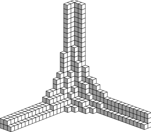
Figure 3: A 3-legged 3-dimensional partition

By a 3-dimensional partition with legs, we mean an object of kind shown in Figure 3. These correspond bijectively to $\mathsf{A}$-fixed $1$-dimensional ideals in $\mathscr{O}_{\mathbb{C}^{3}}$. An $\mathsf{A}$-fixed ideal sheaf on a general toric $X$ is described by a collection $\{\pi_{v}\}$ of 3-dimensional partitions placed at the vertices of $\Delta(X)$ that glue along the edges of $\Delta(X)$. Additionally, nontrivial legs are not allowed along unbounded edges of $\Delta(X)$. These rules are illustrated in Figure 4.

8.1.3

The description of $\operatorname{\mathsf{PT}}(X)^{\mathsf{A}}$ is very similar, see [31]. We discuss localization on the Hilbert scheme here, because we want to make contact with the refined vertex of Iqbal, Kozcaz, and Vafa [18].

Since $\operatorname{Hilb}(X)$ is never compact, Proposition 7.4 may not be directly applied to it. However, if $\operatorname{\mathsf{PT}}(X)$ is compact and if we assume the conjectural formula (16), then the only chamber dependence of the refined invariants comes from the Hilbert scheme of points of $X$.

We have

$$\chi\left(X,\mathscr{K}_{X}^{1/2}\otimes(TX+\mathscr{K}_{X}-T^{*}X-\mathscr{K}_{X}^{*})\right)=\sum_{x\in X^{\mathsf{T}}}\rho(T_{x}X)$$

and hence by Conjecture 2 we have

$$\lim_{z\to 0}\,\chi\left(\operatorname{Hilb}(X,\textup{points}),\widetilde{\mathscr{O}}_{\textup{vir}}\right)\Big{|}_{t\sigma(z)}=\\ {\mathsf{S}}^{\raisebox{1.42262pt}{$\scriptscriptstyle\bullet$}}\frac{q}{(1-q\boldsymbol{\kappa}^{1/2})(1-q\boldsymbol{\kappa}^{-1/2})}\sum_{x\in X^{T}}\left(-\boldsymbol{\kappa}^{1/2}\right)^{\mathsf{ind}_{\sigma}(x)}\,,$$ (65)

for any homomorphism $\sigma:\mathbb{C}^{\times}\to\mathsf{A}$, where

$$\mathsf{ind}_{\sigma}(x)=\dim(T_{x}X)_{+}-\dim(T_{x}X)_{-}=\pm 1$$

is the index of $x\in X^{T}$ with respect to $\sigma$. The sum over $x$ in (65) is an equivariant analog of the Poincaré polynomial of $X$; it jumps across the walls in $\operatorname{Lie}A$ dual to the noncompact edges of toric diagram.

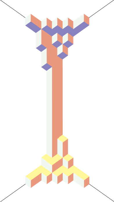
Figure 4: An $\mathsf{A}$-fixed ideal sheaf on $\mathscr{O}(-1)\oplus\mathscr{O}(-1)\to\mathbb{P}^{1}$

8.2 Virtual tangent spaces at fixed points

8.2.1

For a $\mathsf{T}$-fixed ideal sheaf $\mathscr{I}$ on a 3-fold $X$ we denote

$$\mathscr{N}(\mathscr{I})=\chi(\mathscr{O}_{X})-\chi(\mathscr{I},\mathscr{I})\,.$$

For $\mathscr{I}\in\operatorname{Hilb}(X)^{\mathsf{T}}$ this is the virtual tangent (and virtual normal) space at $\mathscr{I}$. For a $1$-dimensional monomial ideal

$$I\subset\mathbb{C}[x_{1},x_{2},x_{3}]=\mathscr{O}_{\mathbb{C}^{3}}$$

the character of $\mathscr{N}(I)$ is well-defined as an element of

$$\mathscr{N}(I)\in\mathbb{Q}(\mathsf{T})\supset K_{\mathsf{T}}(\textup{pt})\,.$$

In fact, the only poles of $\operatorname{tr}_{\mathscr{N}(I)}$ are first-order poles along the weights $t_{i}$ of the directions of infinite legs, see [24]. For any $\mathscr{I}$ we have

$$\mathscr{N}(\mathscr{I})=\sum_{x\in X^{\mathsf{T}}}\mathscr{N}(I_{x})\,,$$

where $I_{x}$ is the restriction of $\mathscr{I}$ to the toric chart at $x$, see [24].

8.2.2

The residue of $\operatorname{tr}_{\mathscr{N}(I)}$ at $t_{1}=1$ only depends on the saturation

$$I^{\textup{leg}}_{1}\supset I$$

of $I$ with respect to $x_{1}$. Combinatorially, $I^{\textup{leg}}_{1}$ corresponds to a pure infinite leg in the direction of $x_{1}$ with the same cross-section $\lambda$ as $I$. We have

$$\mathscr{N}(I^{\textup{leg}}_{1})=\mathbb{C}[x_{1}]\otimes T_{I_{\lambda}}\operatorname{Hilb}(\mathbb{C}^{2})\,,$$

where $I_{\lambda}\subset\mathbb{C}[x_{2},x_{3}]$ is the corresponding monomial ideal.

If $e$ is an edge of $\Delta(X)$ that joins two vertices $x$ and $x^{\prime}$, then the corresponding saturations $I^{e}_{x}$ and $I^{e}_{x^{\prime}}$ glue to form an ideal sheaf $\mathscr{I}^{e}$. Its deformations and obstructions are easy to understand using the formula

$$\mathscr{N}(\mathscr{I}^{e})=\mathscr{N}(I^{e}_{x})+\mathscr{N}(I^{e}_{x^{\prime}})$$

and the explicit description of $T_{I_{\lambda}}\operatorname{Hilb}(\mathbb{C}^{2})$ in terms of arms and legs of the squares of $\lambda$.

8.2.3

We set

$$\mathscr{N}_{\textup{vtx}}(I)=\mathscr{N}(I)-\sum_{i=1}^{3}\mathscr{N}(I^{\textup{leg}}_{i})\in K_{\mathsf{T}}(\textup{pt})\,.$$

It satisfies

$$\mathscr{N}_{\textup{vtx}}(I)=-\mathbb{C}(\boldsymbol{\kappa})\otimes\mathscr{N}_{\textup{vtx}}(I)^{\vee}\,.$$

By construction,

$$\mathscr{N}(\mathscr{I})=\sum_{\textup{edges $e$}}\mathscr{N}(\mathscr{I}^{e})+\sum_{\textup{vertices $x$}}\mathscr{N}_{\textup{vtx}}(I_{x})\,.$$

Since the first term here is explicit, we focus on the vertex contribution.

8.2.4 The K-theoretic vertex

From Proposition 7.3 we have the following formula for the localization vertex:

$$\mathsf{V}(\lambda,\mu,\nu)=\sum_{\pi}(-q)^{|\pi|}\,\rho\left(\mathscr{N}_{\textup{vtx}}(I)_{+}\right)\,,$$ (66)

where the sum is over all $3$-legged partitions $\pi$ ending on given triple $(\lambda,\mu,\nu)$ of $2$-dimensional partitions, $I\in\mathscr{O}_{\mathbb{C}^{3}}$ is the corresponding ideal, and the size of an infinite partition $\pi$ is defined as a rank

$$|\pi|=\operatorname{rk}\left(-2\mathscr{O}-I+\sum I^{\textup{leg}}_{i}\right)$$

of a finite-dimensional virtual $\mathsf{T}$-module. Note this size may be negative. The decomposition

$$\mathscr{N}_{\textup{vtx}}(I)=\mathscr{N}_{\textup{vtx}}(I)_{+}-\mathbb{C}(\boldsymbol{\kappa})\otimes\mathscr{N}_{\textup{vtx}}(I)^{\vee}_{+}$$

is with respect to sign of the weights on $d\sigma\in\operatorname{Lie}\mathsf{A}$, where $\sigma:\mathbb{C}^{\times}\to\mathsf{A}$ is generic $1$-parameter subgroup. The product $\rho\left(\mathscr{N}_{\textup{vtx}}(I)_{+}\right)$ is independent of the choice of $\sigma$.

8.2.5 The index vertex

We now compute the limit of (66) on $t\sigma(z)\in\mathsf{T}$ as $z\to 0$. This does depend on the choice of $\sigma$ which we call the choice of a slope since $\mathsf{A}$ is 2-dimensional. Because we want the slope to be generic, we choose is so that

$$\mathbb{Q}_{>0}\cdot d\sigma=\mathbb{Q}_{>0}\cdot\left(d\sigma_{0}+\textup{small perturbation}\right)$$ (67)

for some fixed rational slope $d\sigma_{0}$ and an infinitesimal perturbation of a given sign. Given a generic slope like this, we define

$$\mathsf{V}^{\sigma}(\lambda,\mu,\nu) =\lim_{z\to 0}\,\mathsf{V}(\lambda,\mu,\nu)\big{|}_{t\sigma(z)}$$ (68)

$$=\sum_{\pi}(-q)^{|\pi|}\,(-\boldsymbol{\kappa}^{1/2})^{\mathsf{ind}_{\sigma}I}\,,$$

where

$$\mathsf{ind}_{\sigma}I=\operatorname{rk}\mathscr{N}_{\textup{vtx}}(I)_{+}\,.$$ (69)

This jumps as the sign of the small perturbation in (67) changes, that is, as the ray $\mathbb{Q}_{>0}\cdot d\sigma$ crosses from one side of $\mathbb{Q}_{>0}\cdot d\sigma_{0}$ to the other. This wall-crossing is analyzed in [2].

8.3 The refined vertex

8.3.1

We call a slope $\sigma$ preferred if $\sigma_{0}$ fixes one of the coordinate axes. By convention, we choose this to be the $x_{3}$-axis which we plot vertically. In this section, we show that for preferred slopes the index vertex specializes to the refined vertex of [18].

For a general slope, the index (69) is a quite complicated function of a 3-dimensional partition because the character of $\mathscr{N}_{\textup{vtx}}(I)$ depends quadratically on the character of $I$ itself. For preferred slopes, however, there is a big cancellation in $\operatorname{rk}\mathscr{N}_{\textup{vtx}}(I)_{+}$ and the dependence becomes linear, that is, the index may be computed a certain single sum over the boxes $\textup{\char 114}\in\pi$.

8.3.2

Let $\pi$ be a 3-dimensional partition, let $\pi^{\textup{leg}}_{3}$ its leg in the preferred direction, and let $\lambda$ the corresponding $2$-dimensional partition. We view the diagram as a collection of squares $\lambda\subset\mathbb{R}_{\geq 0}^{2}$ in the plane and denote by

$$f_{\lambda}=\textup{boundary}\left(\mathbb{R}_{\geq 0}^{2}\setminus\lambda\right)$$

the profile of $\lambda$. This is a zig-zag line going from $x_{1}$-axis to the $x_{2}$-axis. We label its two possible slopes by the corresponding variable $x_{i}$ and call its corners peaks and valleys, so that that

$$f_{\varnothing}=\{x_{1}\geq 0,x_{2}=0\}\cup\{x_{1}=0,x_{2}\geq 0\}$$

has one valley and no peaks. See (76) below for a more formal definition.

8.3.3

There is a natural projection

$$p:\mathbb{R}^{3}\to f_{\lambda}$$

along the $(1,1,0)$ and $(0,0,1)$ directions. For a box $\textup{\char 114}\in\pi$ we define

$$\xi_{\lambda}(\textup{\char 114})=\begin{cases}x_{1}\,,&p(\textup{\char 114})\in\textup{$x_{1}$-slope of $f_{\lambda}$}\,,\\ x_{2}\,,&p(\textup{\char 114})\in\textup{$x_{2}$-slope of $f_{\lambda}$}\,,\\ x_{3}^{\pm 1}\,,&p(\textup{\char 114})\in\textup{peak/valley of $f_{\lambda}$}\,.\end{cases}$$

This is illustrated in Figure 5. We define

$$\Xi(\pi)=\sum_{\textup{\char 114}\in\pi\setminus\pi^{\textup{leg}}_{3}}\xi_{\lambda}(\textup{\char 114})-\sum_{\textup{\char 114}\in\pi^{\textup{leg}}_{1}}\xi_{\varnothing}(\textup{\char 114})-\sum_{\textup{\char 114}\in\pi^{\textup{leg}}_{2}}\xi_{\varnothing}(\textup{\char 114})\,,$$ (70)

which is a finite sum.

For a preferred slope, the index is computed in the following

Theorem 2.

If $x_{3}$ is fixed by $\sigma_{0}$ then

$$\mathsf{ind}_{\sigma}I=\operatorname{rk}\left(\Xi-\Xi^{\vee}\right)_{+}\,.$$

Of course, one should always bear in mind that the $\mathsf{T}$-weight of the monomials $x_{i}$ are the opposite of the weights of coordinate directions.

8.3.4

The proof of Theorem 2 will take several steps. The first step is to reduce to the case

$$\pi^{\textup{leg}}_{1}=\pi^{\textup{leg}}_{2}=\varnothing\,.$$ (71)

Introduce the following truncation

$$I_{N}=I+(x_{1}^{N},x_{2}^{N})\,,$$

and the corresponding truncations $I^{\textup{leg}}_{i,N}$ of the saturations $I^{\textup{leg}}_{i}$. The general case of Theorem 2 is reduced to (71) by the following

Lemma 8.1.

We have

$$\mathsf{ind}_{\sigma}=\operatorname{rk}\left(\mathscr{N}_{\textup{vtx}}(I_{N})-\mathscr{N}_{\textup{vtx}}(I^{\textup{leg}}_{1,N})-\mathscr{N}_{\textup{vtx}}(I^{\textup{leg}}_{2,N})\right)_{+}$$

for all $N\gg 0$.

Proof.

Denote by $Z$ the spectrum of $\mathscr{O}/I$ so that

$$\mathscr{O}_{Z_{N}}=\mathscr{O}_{Z}-x_{1}^{N}\mathscr{O}_{Z^{\textup{leg}}_{1}}-x_{2}^{N}\mathscr{O}_{Z^{\textup{leg}}_{2}}\,.$$

We compute

$$\mathscr{N}_{\textup{vtx}}(I)-\mathscr{N}_{\textup{vtx}}(I_{N})+\mathscr{N}_{\textup{vtx}}(I^{\textup{leg}}_{1,N})+\mathscr{N}_{\textup{vtx}}(I^{\textup{leg}}_{2,N})=\\ -\chi\left(\mathscr{O}_{Z_{N}\setminus Z^{\textup{leg}}_{1,N}},x_{1}^{N}\mathscr{O}_{Z^{\textup{leg}}_{1}}\right)-\chi\left(\mathscr{O}_{Z_{N}\setminus Z^{\textup{leg}}_{2,N}},x_{2}^{N}\mathscr{O}_{Z^{\textup{leg}}_{2}}\right)\\ -\chi\left(x_{1}^{N}\mathscr{O}_{Z^{\textup{leg}}_{1}},x_{2}^{N}\mathscr{O}_{Z^{\textup{leg}}_{2}}\right)-\dots{}$$ (72)

where dots stand for 3 more terms obtained by reversing the order of entries in Euler characteristic. Since the supports of all pairs in (72) extend along different coordinate axes, each Euler characteristic is a zero-dimensional element of $K_{\mathsf{T}}(\textup{pt})$ shifted by a large nontrivial weight of $\sigma_{0}$. Therefore, it makes no contribution to the index. ∎

8.3.5 The balance lemma

One can think about the situation (71) a bit more abstractly. Let $C$ be a 1-dimensional component of $X^{\sigma_{0}}$ for some general 3-fold $X$, the case at hand being the $x_{3}$-axis in $X=\mathbb{C}^{3}$. Let $Z$ be a $\mathsf{A}$-invariant subscheme contained in an infinitesimal neighborhood of $C$ and let $E\subset Z$ be the closure of the generic point of $Z$ along $C$, for example

$$E=Z^{\textup{leg}}_{3}$$

in our concrete situation. We define

$$\Xi_{Z}=\chi\!\left(\mathscr{I}_{E},\mathscr{O}_{Z\setminus E}\otimes\left(\pi^{*}TC\right)^{\otimes{N}}\right)\,,$$ (73)

where $TC$ is the tangent bundle of $C$, $\pi:Z\to C$ is the $\mathsf{T}$-equivariant projection, and

$$0\ll N\ll\|\textup{small perturbation}\|^{-1}$$

where the small perturbation refers to (67).

The following technical result compares the deformations of $Z$ with the deformations of $E$, showing that the index of the difference is linear in $[\mathscr{O}_{Z}]$.

Lemma 8.2.

We have

$$\operatorname{rk}\left(\mathscr{N}(Z)-\mathscr{N}(E)\right)_{+}=\operatorname{rk}\left(\Xi_{Z}-\Xi_{Z}^{\vee}\right)_{+}\,.$$ (74)

The proof of this lemma is given in the Appendix. It is clear that the Lemma proves the theorem modulo checking that the definition (73) specializes to the formula (70).

8.3.6 Conclusion of the proof

We are now back in the case $X=\mathbb{C}^{3}$, $C$ is the $x_{3}$-axis, and $I_{E}=I^{\textup{leg}}_{3}$ is generated by monomials in $x_{1}$ and $x_{2}$. Concretely,

$$I_{E}=\left(\left\{x_{1}^{i}x_{2}^{j}\right\}_{(i,j)\notin\lambda}\right)$$

where $\lambda\in\mathbb{Z}_{\geq 0}\times\mathbb{Z}_{\geq 0}$ is the diagram of a partition. For example, the case

$$I_{E}=(x_{1}^{2},x_{2}^{3})$$

is depicted in Figure 5. Visually, one may compare $E$ to a chimney in the corner of a room and then $Z$ corresponds to a few boxes stacked against this chimney (in violation of all building regulations), as in Figure 5.

Figure 5: The function $\xi_{\lambda}(\textup{\char 114})$

The generators and relations for the ideal $I_{E}$ correspond to the inner and outer corners of the chimney, that is, to the valleys and the peaks of the profile of $\lambda$. In our example, we have generators of degree $x_{1}^{2}$ and $x_{2}^{3}$, together with a relation of degree $x_{1}^{2}x_{2}^{3}$. In general, let us denote by

$$\gamma_{i},\rho_{i}\in\mathbb{Z}_{\geq 0}^{2}\subset\mathbb{Z}^{3}$$

the multiindex degrees of generators and relations of $I_{E}$. The we have an equivariant free resolution

$$0\to\bigoplus_{i=1}^{g-1}x^{\rho_{i}}\mathscr{O}_{\mathbb{C}^{3}}\to\bigoplus_{i=1}^{g}x^{\gamma_{i}}\mathscr{O}_{\mathbb{C}^{3}}\to I_{E}\to 0$$ (75)

where $g$ is the number of the generators (number of inner corners).

Since the $\mathsf{A}$-weight of $x_{3}\in T^{*}C$ is minus the weight of $TC$, the contribution of a monomial $x^{\textup{\char 114}}\in\mathscr{O}_{Z\setminus E}$ to the index of $\Xi_{Z}$ equals the $\sigma$-index of the following $\mathsf{A}$-module

$$\Xi_{\textup{\char 114}}=x_{3}^{-N}\sum_{i=1}^{g}{x^{\textup{\char 114}-\gamma_{i}}}+x_{3}^{N}\sum_{i=1}^{g-1}{x^{\rho_{i}-\textup{\char 114}}}\,.$$

This index is computed as follows. We may assume

$$d\sigma=x_{1}\frac{\partial}{\partial x_{1}}-x_{2}\frac{\partial}{\partial x_{2}}\,.$$

Consider the function

$$c((a_{1},a_{2},a_{3}))=a_{1}-a_{2}\,.$$

Clearly, $d\sigma_{0}\cdot x^{\textup{\char 114}}=c(\textup{\char 114})\,x^{\textup{\char 114}}$. The level sets of $c(\textup{\char 114})$ are the diagonal slices in Figure 5. Let $f_{\lambda}(s)$ be the profile of $\lambda$, defined by

$$\tfrac{1}{2}f^{\prime\prime}_{\lambda}=\sum\delta_{c(\gamma_{i})}-\sum\delta_{c(\rho_{i})}\,,$$ (76)

together with

$$f_{\lambda}(s)=|s|\,,\quad|s|\gg 0\,.$$

Then

$$\mathsf{ind}_{\sigma}\Xi_{\textup{\char 114}}=f^{\prime}_{\lambda}(c(\textup{\char 114}))$$

extended by left or right continuity depending on the weight of $x_{3}$. This is color-coded in Figure 5. Clearly,

$$\mathsf{ind}_{\sigma}\Xi_{\textup{\char 114}}=\xi_{\lambda}(\textup{\char 114})$$

which concludes the proof.

Appendix A Appendix

A.1 Proof of the balance lemma

A.1.1

Since $\mathscr{O}_{Z}/\mathscr{O}_{E}$ is zero-dimensional, the statement of Lemma 8.2 is purely local and we can assume we are in the situation of Section 8.3.6.

We begin we the special case $E=\varnothing$, so that $\mathscr{N}(E)=0$. We need to show

$$\mathscr{N}(Z)\equiv x_{3}^{-N}\,\chi(\mathscr{O}_{Z})-x_{3}^{N}\,\overline{\chi(\mathscr{O}_{Z})}$$ (77)

for all sufficiently large $N$ and the relation $\equiv$ on $\mathsf{A}$-modules means that they have the same $\sigma$-index.

A.1.2

In fact, it suffices to take $N$ so that $x_{3}^{N}\in\mathscr{I}_{Z}$, in other words, that $N$ is larger than the height of the stack of boxes corresponding to $Z$. As we will see, the difference between the left-hand side and the right-hand side of (77) corresponds to the deformations of

$$\mathscr{F}=\pi_{12*}\left(\mathscr{I}_{Z}/x_{3}^{N}\right)\,.$$

Here $\pi_{12}$ is the projection onto the $(x_{1},x_{2})$-plane and $\pi_{12*}$ means that we view $\mathscr{I}_{Z}/x_{3}^{N}$ as a $\mathscr{O}_{\mathbb{C}^{2}}=\mathbb{C}[x_{1},x_{2}]$ module, that is as a (degenerate) framed rank $N$ instanton on $\mathbb{C}^{2}$.

Away from the origin of $\mathbb{C}^{2}$, $\mathscr{F}$ is the same as

$$\mathscr{F}_{\varnothing}=\sum_{i=0}^{N-1}x_{3}^{i}\,\mathscr{O}_{\mathbb{C}^{2}}\,.$$

The $\mathsf{A}$-action on the $x_{3}$ is thus transformed into into the action on the framing of $\mathscr{F}$.

A.1.3

Moduli of framed torsion-free sheaves on $\mathbb{C}^{2}$ is a smooth manifold with tangent space

$$\mathscr{N}_{2}(Z)=\chi_{\mathbb{C}^{2}}(\mathscr{F}_{\varnothing},\mathscr{O}_{Z})+\chi_{\mathbb{C}^{2}}(\mathscr{O}_{Z},\mathscr{F}_{\varnothing})-\chi_{\mathbb{C}^{2}}(\mathscr{O}_{Z},\mathscr{O}_{Z})\,,$$ (78)

where $\chi_{\mathbb{C}^{2}}$ means we treat all sheaves as $\mathsf{A}$-equivariant $\mathscr{O}_{\mathbb{C}^{2}}$-modules. In particular,

$$\chi_{\mathbb{C}^{2}}(\mathscr{O}_{0},\mathscr{O}_{0})=(1-x_{1}^{-1})(1-x_{2}^{-1})=(1-x_{3}^{-1})^{-1}\,\chi(\mathscr{O}_{0},\mathscr{O}_{0})$$

where $0\in\mathbb{C}^{2}\subset\mathbb{C}^{3}$ is the origin. It follows that

$$\mathscr{N}(Z)=(1-x_{3}^{-1})\,\mathscr{N}_{2}(Z)+x_{3}^{-N}\,\chi(\mathscr{O}_{Z})-x_{3}^{N}\,\overline{\chi(\mathscr{O}_{Z})}$$

Therefore, (77) is equivalent to showing

$$\mathsf{ind}_{\sigma}\,\mathscr{N}_{2}(Z)=0$$ (79)

A.1.4

The symplectic form $dx_{1}\wedge dx_{2}$ on $\mathbb{C}^{2}$ induces a symplectic form on instanton moduli and, in particular, a symplectic form $\omega_{\mathscr{F}}$ on tangent space $\mathscr{N}_{2}(\mathscr{F})$ to $\mathscr{F}$. The torus $\mathsf{A}$ scales this symplectic form with the weight of $x_{1}x_{2}$, which is the same as the weight of $x_{3}^{-1}$. Therefore, $\omega_{\mathscr{F}}$ pairs attracting and repelling direction with the exception of the weights $0$ and $x_{3}^{-1}$. Therefore (79) follows from the following

Lemma A.1.

$$\mathscr{N}_{2}(Z)^{\mathsf{A}}=0\,.$$

Proof.

We have

$$\mathscr{F}=\bigoplus_{i=1}^{N}x_{3}^{i-1}\,\mathscr{I}_{\lambda^{(i)}}$$

where $\mathscr{I}_{\lambda}\subset\mathbb{C}[x_{1},x_{2}]$ is a monomial ideal corresponding to a partition $\lambda$ and

$$\lambda^{(1)}\supset\lambda^{(2)}\supset\dots\supset\lambda^{(N)}\,.$$

Therefore

$$\mathscr{N}_{2}(Z)=\sum_{i,j}x_{3}^{j-i}\left(\chi_{\mathbb{C}^{2}}(\mathscr{O}_{\mathbb{C}^{2}})-\chi_{\mathbb{C}^{2}}\left(\mathscr{I}_{\lambda^{(i)}},\mathscr{I}_{\lambda^{(j)}}\right)\right)$$

The claim then follows from the following Lemma A.2. ∎

A.1.5

Lemma A.2.

Let $\mathscr{I},\mathscr{J}\in\mathbb{C}[x_{1},x_{2}]$ be monomial ideals. If

$$(n<0\textup{ and }\mathscr{I}\supset\mathscr{J})\textup{ or }(n\geq 0\textup{ and }\mathscr{I}\subset\mathscr{J})$$

then the weight $(x_{1}x_{2})^{n}$ does not occur in

$$\chi_{\mathbb{C}^{2}}(\mathscr{O}_{\mathbb{C}^{2}})-\chi_{\mathbb{C}^{2}}\left(\mathscr{I},\mathscr{J}\right)\,.$$

Proof.

By duality, it suffices to consider the case $\mathscr{I}\supset\mathscr{J}$. From a resolution like (75), we have

$$\operatorname{supp}\,\chi_{\mathbb{C}^{2}}\left(\mathscr{I},\mathscr{J}\right)\subset\bigcup_{i,j}\operatorname{supp}\,\,x^{b_{j}-a_{j}}\mathscr{O}_{\mathbb{C}^{2}}\,,$$ (80)

where

$$\{a_{i}\},\{b_{j}\}\subset(\mathbb{Z}_{\geq 0})^{2}$$

are the degrees of generators and relations for $I$ and $J$, respectively, and by support of a $\mathsf{A}$-module we mean the support of its Fourier transform, that is, the set of weights that occur in it.

The inclusion $\mathscr{I}\supset\mathscr{J}$ obviously implies

$$b_{j}-a_{i}\notin(\mathbb{Z}_{<0})^{2}$$

and hence all supports in (80) are disjoint from $(\mathbb{Z}_{<0})^{2}$. ∎

This completes the proof of (77).

A.1.6

We now deduce the general case of Lemma 8.2 from its special case (77). Choose $N$ so large that $x_{3}^{N}$ annihilates $\mathscr{O}_{Z\setminus E}$. Expanding $\mathscr{N}$ using

$$\left[\mathscr{O}_{Z}\right]=\left[\mathscr{O}_{Z\setminus E}\right]+\left[\mathscr{O}_{E}/x_{3}^{N}\right]+x_{3}^{N}\left[\mathscr{O}_{E}\right]$$

we get

$$\mathscr{N}(Z)-\mathscr{N}(E)=\mathscr{N}(Z/x_{3}^{N})-\mathscr{N}(E/x_{3}^{N})-\operatorname{\textsf{Alt}}\,x_{3}^{-N}\chi(\mathscr{O}_{E},\mathscr{O}_{Z\setminus E})\,.$$ (81)

where, by definition,

$$\operatorname{\textsf{Alt}}V=V-V^{\vee}$$

for any $\mathsf{A}$-module $V$. From (77) we conclude

$$\mathscr{N}(Z/x_{3}^{N})-\mathscr{N}(E/x_{3}^{N})\equiv\operatorname{\textsf{Alt}}x_{3}^{-N}\chi(\mathscr{O}_{\mathbb{C}^{3}},\mathscr{O}_{Z\setminus E})\,.$$

This concludes the proof.

Nikita Nekrasov
Simons Center for Geometry and Physics
Stony Brook University, Stony Brook NY 11794-3636, U.S.A.
nikitastring@gmail.com

Andrei Okounkov
Department of Mathematics, Columbia University
New York, NY 10027, U.S.A.

Institute for Problems of Information Transmission
Bolshoy Karetny 19, Moscow 127994, Russia

Laboratory of Representation Theory and Mathematical Physics
Higher School of Economics
Myasnitskaya 20, Moscow 101000, Russia

References

- [1] M. Aganagic, A. Klemm, M. Mariño, C. Vafa, The topological vertex, Comm. Math. Phys. 254 (2005), no. 2, 425–-478.
- [2] M. Aganagic and A. Okounkov, in preparation.
- [3] I. Antoniadis, E. Gava, K. S. Narain and T. R. Taylor, Nucl. Phys. B 413, 162 (1994) [hep-th/9307158].
- [4] E. Arbarello, M. Cornalba, P. Griffiths, J. Harris, Geometry of algebraic curves, Vol. I. Grundlehren der Mathematischen Wissenschaften, 267, Springer, 1985.
- [5] J. Bagger, N. Lambert, S. Mukhi, C. Papageorgakis, Multiple membranes in M-theory, Phys. Rep. 527 (2013), no. 1, 1–-100.
- [6] D. Barlet, Espace analytique réduit des cycles analytiques complexes compacts d’un espace analytique complexe de dimension finie, Lecture Notes in Math., 482, 1975.
- [7] K. Behrend, J. Bryan, and B. Szendröi, Motivic degree zero Donaldson-Thomas invariants, Invent. Math. 192 (2013), no. 1, 111–-160.
- [8] M. Bershadsky, S. Cecotti, H. Ooguri and C. Vafa, Commun. Math. Phys. 165, 311 (1994) [hep-th/9309140].
- [9] V. Bussi, D. Joyce, S. Meinhardt, On motivic vanishing cycles of critical loci, arXiv:1305.6428.
- [10] R. Bott and C. Taubes, On the rigidity theorems of Witten, J. Amer. Math. Soc. 2 (1989), no. 1, 137–186.
- [11] J. Choi, S. Katz, A. Klemm, The refined BPS index from stable pair invariants, arXiv:1210.4403.
- [12] B. Fantechi and L. Göttsche, Riemann-Roch theorems and elliptic genus for virtually smooth schemes, Geom. Topol. 14 (2010), no. 1, 83–-115.
- [13] T. Graber and R. Pandharipande, Localization of virtual classes, Invent. Math. 135 (1999), no. 2, 487–-518.
- [14] A. Haupt, A. Lukas, K. Stelle, M-theory on Calabi-Yau five-folds, J. High Energy Phys. 2009, no. 5.
- [15] M. O. Hønsen, A compact moduli space for Cohen-Macaulay curves in projective space, Ph.D. Thesis, MIT, 2004.
- [16] C. M. Hull, Gravitational duality, branes and charges, Nucl. Phys. B 509, 216 (1998) [hep-th/9705162].
- [17] A. Iqbal, N. Nekrasov, A. Okounkov and C. Vafa, Quantum foam and topological strings, JHEP 0804, 011 (2008) [hep-th/0312022].
- [18] A. Iqbal, C. Kozçaz, C. Vafa, The refined topological vertex, J. High Energy Phys. 2009, no. 10.
- [19] A. J. de Jong and A. Okounkov, in preparation.
- [20] J. Kollár, Rational curves on algebraic varieties, Ergebnisse der Mathematik und ihrer Grenzgebiete, 32, Springer, 1996.
- [21] M. Kontsevich and Y. Soibelman, Stability structures, motivic Donaldson-Thomas invariants and cluster transformations, arXiv:0811.2435.
- [22] A. Losev, G. W. Moore and S. L. Shatashvili, M & m’s, Nucl. Phys. B 522, 105 (1998) [hep-th/9707250].
- [23] D. Maulik, Motivic residues and DT theory, in preparation.
- [24] D. Maulik, N. Nekrasov, A. Okounkov, R. Pandharipande, Gromov-Witten theory and Donaldson-Thomas theory, I and II, Compos. Math. 142 (2006), no. 5, 1263-1304.
-
[25]
N. Nekrasov,
A la recherche de la M-theorie perdue.
-theory: chasing theory,
Strings’2004,
Comptes Rendue Physique 6 (2005), no. 2, pp. 261-269
hep-th/0412021. - [26] N. Nekrasov, Instanton partition functions and M-theory, 5th Takagi Lectures, 2008, Japanese Journal of Mathematics Volume 4 (2009), Issue 1 , pp 63-93
- [27] N. Nekrasov, Five dimensional gauge theories and relativistic integrable systems, Nucl. Phys. B 531, 323 (1998) [hep-th/9609219].
- [28] N. Nekrasov and A. S. Schwarz, Instantons on noncommutative and -superconformal six-dimensional theory, Commun. Math. Phys. 198, 689 (1998) [hep-th/9802068].
- [29] A. Okounkov, N. Reshetikhin, C Vafa, Quantum Calabi-Yau and classical crystals, The unity of mathematics, 597–-618, Progr. Math., 244, Birkhäuser, 2006.
- [30] R. Pandharipande and R. Thomas, Curve counting via stable pairs in the derived category, Invent. Math. 178 (2009), no. 2, 407–-447.
- [31] R. Pandharipande and R. Thomas, The 3-fold vertex via stable pairs, Geom. Topol. 13 (2009), no. 4, 1835–-1876.
- [32] Quantum fields and strings: a course for mathematicians, Vol. 1 & 2. Material from the Special Year on Quantum Field Theory held at the Institute for Advanced Study. Edited by Pierre Deligne, Pavel Etingof, Daniel S. Freed, Lisa C. Jeffrey, David Kazhdan, John W. Morgan, David R. Morrison and Edward Witten, 1999.
- [33] A. Sen, Dynamics of multiple Kaluza-Klein monopoles in M and string theory, Adv. Theor. Math. Phys. 1, 115 (1998) [hep-th/9707042].
- [34] R. Thomas, A holomorphic Casson invariant for Calabi–Yau -folds and bundles on K3 fibrations, J. Differential Geom. 54 (2000), 367–-438.
- [35] E. Witten, String theory dynamics in various dimensions, Nucl. Phys. B 443, 85 (1995) [hep-th/9503124].
- [36] E. Witten, BPS Bound states of D0-D6 and D0-D8 systems in a B field, JHEP 0204, 012 (2002) [hep-th/0012054].
- [37] E. Witten, Elliptic Genera and Quantum Field Theory, Commun. Math. Phys. 109, 525 (1987).
- [38] E. Witten, Supersymmetry and Morse theory, J. Differential Geom. 17 (1982), no. 4, 661–-692.