Adaptive Time Discretization for Retarded Potentials

Abstract

In this paper, we will present advanced discretization methods for solving retarded potential integral equations. We employ a $C^{\infty}$-partition of unity method in time and a conventional boundary element method for the spatial discretization. One essential point for the algorithmic realization is the development of an efficient method for approximation the elements of the arising system matrix. We present here an approach which is based on quadrature for (non-analytic) $C^{\infty}$ functions in combination with certain Chebyshev expansions.

Furthermore we introduce an a posteriori error estimator for the time discretization which is employed also as an error indicator for adaptive refinement. Numerical experiments show the fast convergence of the proposed quadrature method and the efficiency of the adaptive solution process.

AMS subject classifications: 35L05, 65N38, 65R20.

Keywords: wave equation, retarded potential integral equation, a posteriori error estimation, adaptive solution, numerical quadrature.

1 Introduction

In this paper, we will consider the efficient numerical solution of the wave equation in unbounded domains. The exact solution is represented as a retarded potential and the arising space-time boundary integral equation (RPIE) is solved numerically by using a Galerkin method in time and space ([6], [1], [8]).

The novelties compared to existing methods ([1], [3], [8], [9], [14], [18], [21]) are as follows.

• We employ a $C^{\infty}$-partition of unity enriched by polynomials for the temporal discretization as introduced in [18]. This approach overcomes the technical difficulty to first determine and then to integrate over the intersection of the discrete light cone with the spatial mesh which arises if conventional piecewise polynomial finite elements are employed in time (cf. [9]). However, the arising quadrature problem for our $C^{\infty}$ basis functions is not completely standard since the functions are not analytic. In this paper we will propose an efficient method to approximate the arising integrals and perform systematic numerical experiments to demonstrate its fast convergence. It turns out that for the important range of accuracies $\left[10^{-1},10^{-8}\right]$ the method converges nearly as fast as for analytic integrands.

• We present an a posteriori error estimator for retarded potential integral equations which also is employed as a refinement indicator for an adaptive solution process. To the best of our knowledge this is the first time that an self-adaptive method is proposed for RPIE in 3D (for the 2D case we refer to the thesis [7]; for adaptive versions of the convolution quadrature method we refer to [11] and [12]). The error estimator is based on the estimator which was proposed in [4], [5] for elliptic boundary integral equation. We will present numerical experiments where the solution contains sharp pulses and/or oscillations at different time scales and time windows. Our error indicator captures very well the irregularities in the solution and marks for refinement at the “right” places. These experiments also indicate that a global error estimator in time is essential for setting up an adaptive method since it seems to be quite complicated for a time stepping scheme to detect the regions in the time history which causes the error at the current time step.

  Remark 1.1.

  We emphasize that the long term goal of this research is to develop a space-time a posteriori error estimator and the resulting algorithm should be fully space-time adpative. In this paper we will present a purely temporal a posteriori error estimator. It turns out that this algorithm is able to capture local irregularities with respect to time very well. We expect that a generalization of this estimator to a space-time adaptive method allows to reduce the dimensions of spatial boundary element matrices substantially so that the loss of the Toeplitz structure in the linear system becomes negligible due to the much smaller dimension of the full system matrix. In any case, a reliable a posteriori error estimator is important also for uniform mesh refinement and serves as a computable upper bound for the error which can be used as a stopping criterion.

• We present systematic numerical experiments to understand i) the convergence behavior of the spatial quadrature depending on the distance of the pairs of panels and the width of the discrete light cone, ii) the influence of the spatial quadrature to the overall discretization error as well as the convergence rates with respect to the energy norm, iii) the long term stability behavior of our space-time Galerkin approach also in comparison with the convolution quadrature method ([13]), iv) the performance of the new self-adaptive method which is based on our a posteriori error estimator.

The paper is structured as follows. After the retarded potential integral equation will be introduced in Section 2 we explain its numerical discretization in Section 3 as well as the numerical approximation of the entries of the system matrix. In Section 4, the a posteriori error estimator is formulated and its numerical evaluation is explained. Numerical experiments are presented in Section 5 which give insights in the performance of the various discretization methods and their influence to the overall discretization. The method and its main features are summarized in the concluding Section 6.

2 Integral Formulation of the Wave Equation

Let $\Omega\subset\mathbb{R}^{3}$ be a Lipschitz domain with boundary $\Gamma$. We consider the homogeneous wave equation

$$\partial_{t}^{2}u-\Delta u=0\hskip 8.53581pt\text{in }\Omega\times\left[0,T\right]$$ (2.1a)

with initial conditions

$$u(\cdot,0)=\partial_{t}u(\cdot,0)=0\hskip 8.53581pt\text{in }\Omega$$ (2.1b)

and Dirichlet boundary conditions

$$u=g\hskip 8.53581pt\text{on }\Gamma\times\left[0,T\right]$$ (2.1c)

on a time interval $\left[0,T\right]$ for $T>0$. In applications, $\Omega$ is often the unbounded exterior of a bounded domain. For such problems, the method of boundary integral equations is an elegant tool where this partial differential equation is transformed to an equation on the bounded surface $\Gamma$. We employ an ansatz as a single layer potential for the solution $u$,

$$u(x,t):=S\phi(x,t):=\int_{\Gamma}\frac{\phi(y,t-\|x-y\|)}{4\pi\|x-y\|}d\Gamma_{y},\hskip 8.53581pt\ (x,t)\in\Omega\times\left[0,T\right]$$ (2.2)

with unknown density function $\phi$. $S$ is also referred to as retarded single layer potential due to the retarded time argument $t-\|x-y\|$ which connects time and space variables.

The ansatz (2.2) satisfies the wave equation (2.1a) and the initial conditions (2.1b). Since the single layer potential can be extended continuously to the boundary $\Gamma$, the unknown density function $\phi$ is determined such that the boundary conditions (2.1c) are satisfied. This results in the boundary integral equation for $\phi$,

$$\int_{\Gamma}\frac{\phi(y,t-\|x-y\|)}{4\pi\|x-y\|}d\Gamma_{y}=g(x,t)\hskip 8.53581pt\forall(x,t)\in\Gamma\times\left[0,T\right].$$ (2.3)

In order to solve this boundary integral equation numerically we introduce a weak formulation of (2.3) according to [1, 8]. Therefore we introduce the space

$$H^{-1/2,-1/2}(\Gamma\times[0,T]) :=L^{2}([0,T],H^{-1/2}(\Gamma))+H^{-1/2}([0,T],L^{2}(\Gamma)).$$

A suitable space-time variational formulation of (2.3) is then given by: Find $\phi\in H^{-1/2,-1/2}(\Gamma\times[0,T])$ s.t.

$$a(\phi,\zeta):=\int_{0}^{T}\int_{\Gamma}\int_{\Gamma}\frac{\dot{\phi}(y,t-\|x-y\|)\zeta(x,t)}{4\pi\|x-y\|} d\Gamma_{y}d\Gamma_{x}dt$$

$$=\int_{0}^{T}\int_{\Gamma}\dot{g}(x,t)\zeta(x,t)d\Gamma_{x}dt=:b(\zeta)$$ (2.4)

for all $\zeta\in H^{-1/2,-1/2}(\Gamma\times[0,T])$, where we denote by $\dot{\phi}$ the derivative with respect to time. It can be shown that $a(\cdot,\cdot)$ is coercive in $H^{-1/2,-1/2}(\Gamma\times[0,T])$, i.e.

$$a(\phi,\phi)\geq C\|\phi\|_{H^{-1/2,-1/2}(\Gamma\times[0,T])}^{2}.$$ (2.5)

This, together with an energy argument, can be used to show unconditional stability of conforming Galerkin approximations (cf. [1, 8]) of (2.4).

3 Numerical Discretization

We discretize the variational problem (2.4) using a Galerkin method in space and time. Therefore we replace $H^{-1/2,-1/2}(\Gamma\times[0,T])$ by a finite dimensional subspace $V_{\operatorname{Galerkin}}$ being spanned by some basis functions $\{b_{i}\}_{i=1}^{L}$ in time and some basis functions $\{\varphi_{j}\}_{j=1}^{M}$ in space. This leads to the discrete ansatz

$$\phi_{\operatorname{Galerkin}}(x,t)=\sum_{i=1}^{L}\sum_{j=1}^{M}\alpha_{i}^{j}\varphi_{j}(x)b_{i}(t),\hskip 8.53581pt(x,t)\in\Gamma\times\left[0,T\right]$$ (3.1)

for the approximate solution, where $\alpha_{i}^{j}$ are the unknown coefficients. Plugging (3.1) into the variational formulation (2.4) and using the basis functions $b_{k}$ and $\varphi_{l}$ as test functions leads to the linear system

$$\underline{\underline{\mathbf{A}}}\cdot\underline{\boldsymbol{\alpha}}=\underline{\mathbf{g}},$$

where the block matrix $\underline{\underline{\mathbf{A}}}\in\mathbb{R}^{LM\times LM}$, the unknown coefficient vector $\underline{\boldsymbol{\alpha}}\in\mathbb{R}^{LM}$ and the right-hand side vector $\underline{\mathbf{g}}\in\mathbb{R}^{LM}$ can be partitioned according to

$$\underline{\underline{\mathbf{A}}}:=\begin{bmatrix}\mathbf{A}_{1,1}&\mathbf{A}_{1,2}&\cdots&\mathbf{A}_{1,L}\\ \mathbf{A}_{2,1}&\mathbf{A}_{2,2}&\cdots&\mathbf{A}_{2,L}\\ \vdots&\vdots&\ddots&\vdots\\ \mathbf{A}_{L,1}&\mathbf{A}_{L,2}&\cdots&\mathbf{A}_{L,L}\end{bmatrix},\qquad\underline{\boldsymbol{\alpha}}:=\begin{bmatrix}\boldsymbol{\alpha}_{1}\\ \boldsymbol{\alpha}_{2}\\ \vdots\\ \boldsymbol{\alpha}_{L}\end{bmatrix},\qquad\underline{\mathbf{g}}:=\begin{bmatrix}\mathbf{g}_{1}\\ \mathbf{g}_{2}\\ \vdots\\ \mathbf{g}_{L}\end{bmatrix},$$ (3.2)

with

$$\mathbf{A}_{k,i}\in\mathbb{R}^{M\times M},\quad\boldsymbol{\alpha}_{i}\in\mathbb{R}^{M},\quad\mathbf{g}_{k}\in\mathbb{R}^{M}\quad\text{ for }i,k\in\{1,\cdots,L\}.$$

Their entries are given by

$$\mathbf{A}_{k,i}(j,l)=\int_{0}^{T}\int_{\Gamma}\int_{\Gamma}\frac{\varphi_{j}(y)\,\varphi_{l}(x)}{4\pi\|x-y\|}\,\dot{b}_{i}(t-\|x-y\|)b_{k}(t)\,d\Gamma_{y}d\Gamma_{x}dt$$ (3.3)

and

$$\boldsymbol{\alpha}_{i}(j)=\left(\alpha_{i}^{j}\right)_{j=1}^{M},\quad\mathbf{g}_{k}(l)=\int_{0}^{T}\int_{\Gamma}\dot{g}(x,t)\,\varphi_{l}(x)\,b_{k}(t)d\Gamma_{x}dt$$

respectively. We rewrite (3.3) by introducing a univariate function $\psi_{i,k}$ with

$$\psi_{k,i}(r)=\int_{0}^{T}\dot{b}_{i}(t-r)b_{k}(t)dt$$ (3.4)

and obtain

$$\mathbf{A}_{k,i}(j,l) =\int_{\Gamma}\int_{\Gamma}\frac{\varphi_{j}(y)\,\varphi_{l}(x)}{4\pi\|x-y\|}\psi_{k,i}(\|x-y\|)\,d\Gamma_{y}d\Gamma_{x}$$

$$=\int_{\text{supp}(\varphi_{l})}\int_{\text{supp}(\varphi_{j})}\frac{\varphi_{j}(y)\,\varphi_{l}(x)}{4\pi\|x-y\|}\psi_{k,i}(\|x-y\|)\,d\Gamma_{y}d\Gamma_{x}.$$ (3.5)

The efficient and accurate computation of the matrix entries (3.5) is crucial for this method and represents a major challenge in the space-time Galerkin approach. The choice of the basis functions in time plays here a significant role. In this paper we use smooth and compactly supported temporal shape functions $b_{i}$ in (3.1) whose definition was addressed in [18]. For the sake of a self-contained presentation we briefly recall their definition. Let

$$f\left(t\right):=\left\{\begin{array}[c]{ll}\frac{1}{2}\operatorname{erf}\left(2\operatorname{artanh}t\right)+\frac{1}{2}&\left|t\right|<1,\\ 0&t\leq-1,\\ 1&t\geq 1\end{array}\right.$$

and note that $f\in C^{\infty}\left(\mathbb{R}\right)$. Next, we will introduce some scaling. For a function $g\in C^{0}\left(\left[-1,1\right]\right)$ and real numbers $a<b$, we define $g_{a,b}\in C^{0}\left(\left[a,b\right]\right)$ by

$$g_{a,b}\left(t\right):=g\left(2\frac{t-a}{b-a}-1\right).$$

We obtain a bump function on the interval $\left[a,c\right]$ with joint $b\in\left(a,c\right)$ by

$$\rho_{a,b,c}\left(t\right):=\left\{\begin{array}[c]{ll}f_{a,b}\left(t\right)&a\leq t\leq b,\\ 1-f_{b,c}\left(t\right)&b\leq t\leq c,\\ 0&\text{otherwise.}\end{array}\right.$$

Let us now consider the closed interval $\left[0,T\right]$ and $l$ (not necessarily equidistant) timesteps

$$0=t_{0}<t_{1}<\ldots t_{l-2}<t_{l-1}=T.$$ (3.6)

A smooth partition of unity of the interval $[0,T]$ then is defined by

$$\mu_{1}:=1-f_{t_{0},t_{1}},\quad\mu_{l}:=f_{t_{l-2,l-1}},\quad\forall 2\leq i\leq l-1:\mu_{i}:=\rho_{t_{i-2},t_{i-1},t_{i}}.$$

Smooth and compactly supported basis functions $b_{i}$ in time can then be obtained by multiplying these partition of unity functions with suitably scaled Legendre polynomials (cf. [18] for details):

$$\mu_{1}(t)\cdot 8\cdot\left(\frac{t}{t_{1}}\right)^{2}P_{m-2}\left(\frac{2}{t_{1}}t-1\right)\quad m=2,\ldots,\max(2,p),$$

$$\mu_{i}(t)P_{m}\left(2\frac{t-t_{i-2}}{t_{i}-t_{i-2}}-1\right)\quad m=0,\ldots,p,\hskip 2.84526pti=2,\ldots,l-1,$$ (3.7)

$$\mu_{l}(t)P_{m}\left(2\frac{t-t_{l-2}}{t_{l-1}-t_{l-2}}-1\right)\quad m=0,\ldots,p.$$

We will use the above basis functions in time for the Galerkin approximation in (3.1). The order of the approximation in time can be controlled by $p$ in (3.7). For the choice $p=0$ the solution is approximated in time merely with the partition of unity functions $\mu_{i}$. This corresponds to the approximation with piecewise constant functions in the standard Galerkin approach.
For the discretization in space we use standard piecewise polynomials basis functions $\varphi_{j}$.

3.1 Efficient evaluation of $\psi_{k,i}$

The approximation of the matrix entries using quadrature is the most time consuming part of the method. In order to reduce the computational time, an efficient evaluation of the integrand in (3.5) is crucial. Since $\psi_{k,i}$ consists itself of an integral this evaluation can typically not be done exactly and has to be approximated. One obvious strategy is to apply Gauss-Legendre quadrature also to the integral in $\psi_{k,i}$. In order to obtain accurate results this unfortunately requires a relatively high number of quadrature nodes and furthermore the basis functions $\dot{b_{i}}$ and $b_{k}$ have to be evaluated multiple times which is itself expensive due to the presence of the error function and the inverse hyperbolic tangent.
In order to speed up the evaluation of (3.5) we therefore want to represent $\psi_{k,i}$ accurately by functions that are easy to construct and allow a fast evaluation. Since $\psi_{k,i}$ is smooth and compactly supported we choose piecewise Chebyshev polynomials for this task. We introduce

$$\text{min}_{k}:=\min\operatorname{supp}b_{k}\quad\text{ and }\quad\text{max}_{k}:=\max\operatorname{supp}b_{k}$$

for all $1\leq k\leq L$, so that

$$\operatorname{supp}\psi_{k,i}=[\text{min}_{k}-\text{max}_{i},\text{max}_{k}-\text{min}_{i}]=:[a,b].$$

We divide $[a,b]$ into $m$ subintervals of length

$$h_{m}:=\frac{b-a}{m}$$

and denote

$$\Delta_{m,j}:=[a+(j-1)h_{m},a+jh_{m}]$$

for $j=1,\ldots,m$. We approximate $\psi_{k,i}$ on each subinterval by a linear combination of Chebyshev polynomials $T_{v}$ of degree $v$, i.e.,

$$\psi_{k,i}(r)|_{\Delta_{m,j}}\approx\sum_{v=0}^{q-1}c_{v}T_{v}(\varphi(r))-\frac{1}{2}c_{0},$$ (3.8)

where

$$\varphi:\Delta_{m,j}\rightarrow[-1,1],\quad r\mapsto\frac{2r-(\max\Delta_{m,j}+\min\Delta_{m,j})}{\max\Delta_{m,j}-\min\Delta_{m,j}}$$

is an appropriate scaling function. The coefficients $c_{v}$ are defined by

$$c_{v}=\frac{2}{q}\sum_{k=1}^{q}\psi_{k,i}\left(\varphi^{-1}\left[\cos\left(\frac{\pi(k-0.5)}{q}\right)\right]\right)\cos\left(\frac{\pi v(k-0.5)}{q}\right)\qquad 0\leq v\leq q-1$$

which can be evaluated efficiently using fast cosine transform methods. The evaluation of the Chebyshev approximation (3.8) can be done with Clenshaw’s recurrence formula (cf. [15, Chapter 5.5]).

Remark 3.1.

The approximation of $\psi_{k,i}$ using the piecewise polynomials (3.8) requires the evaluation of $\psi_{k,i}$ at $q\cdot m$ different points. Note that this has to be done only once for each matrix block $\mathbf{A}_{k,i}$. In order to obtain accurate results we therefore use high-order Gauss-Legendre quadrature for the evaluation of $\psi_{k,i}$ at these points.

Numerical experiments indicate that the accuracy of the approximation in (3.8) has a significant impact on the accuracy of the approximation of (3.5) using Gauss-Legendre quadrature. The number of subintervals $m$ and the polynomial degree $q$ of the piecewise approximations (3.8) should therefore be chosen such that the error $\|\psi_{k,i}-\psi_{k,i}^{\text{approx}}\|_{\infty}$ is sufficiently small; in our numerical experiments a threshold of $10^{-8}$ for this error always preserved the asymptotic convergence rates. We have performed numerical experiments to assemble a table with optimal pairs $\left(m,q\right)$ for certain accuracies. As model situations we have considered the (nonuniform) time grid

$$t_{0}=0,\quad t_{1}=2,\quad t_{2}=3,\quad t_{3}=4.5,\quad t_{4}=7$$

and chosen bump functions $\rho_{t_{0},t_{1},t_{2}}$ and $\rho_{t_{2},t_{3},t_{4}}$ as above. Let

$$b_{1}(t):=\rho_{t_{0},t_{1},t_{2}}(t),\quad b_{2}(t):=\rho_{t_{2},t_{3},t_{4}}(t),$$

$$b_{3}(t):=\rho_{t_{0},t_{1},t_{2}}(t)P_{3}\left(2\frac{t-t_{0}}{t_{2}-t_{0}}-1\right),\quad b_{4}(t):=\rho_{t_{2},t_{3},t_{4}}(t)P_{2}\left(2\frac{t-t_{2}}{t_{4}-t_{2}}-1\right)$$

be functions of the type (3.7). Next, we define

$$\psi_{1}:\mathbb{R}\rightarrow\mathbb{R},r\mapsto\int_{0}^{7}\dot{b}_{1}(t-r)b_{2}(t)dt\quad\text{and}\quad\psi_{2}:\mathbb{R}\rightarrow\mathbb{R},r\mapsto\int_{0}^{7}\dot{b}_{3}(t-r)b_{4}(t)dt.$$

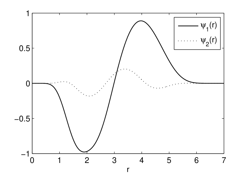
Figure 3.1: $\psi_{1}(r)$ and $\psi_{2}(r)$

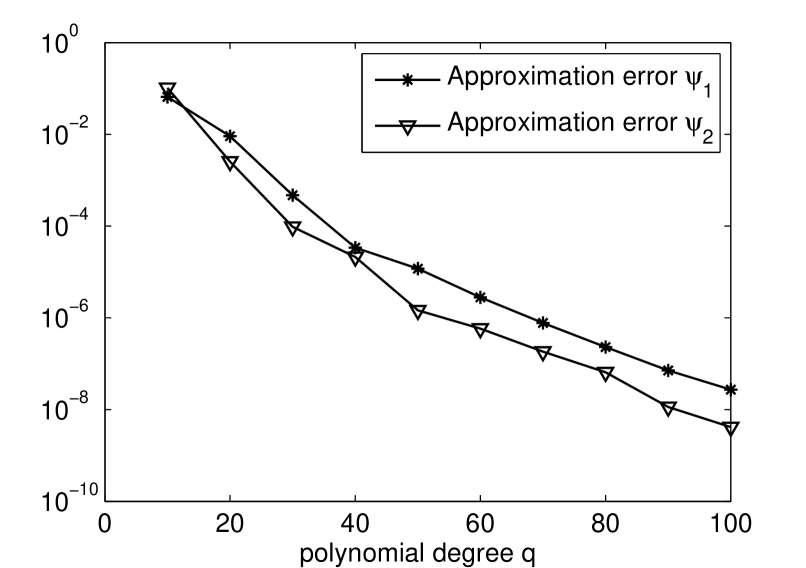
Figure 3.2: $\|\psi_{1}-\psi_{1}^{\text{approx}}\|_{\infty}$ and $\|\psi_{2}-\psi_{2}^{\text{approx}}\|_{\infty}$ in dependence of $q$ for $m=1$.

$\psi_{1}$ and $\psi_{2}$ are illustrated in Figure 3.2. Functions of type $\psi_{2}$ occur in the discretization process if higher order methods in time are used. Although the higher order basis functions $b_{3}$ and $b_{4}$ are more oscillatory than $b_{1}$ and $b_{2}$, Figure 3.2 shows that the corresponding function $\psi_{2}$ is of similar shape than $\psi_{1}$ due to smoothing effect of the integration.
Figure 3.2 shows the error that results from the approximation of $\psi_{1}$ and $\psi_{2}$ with the Chebyshev approximation (3.8) of different polynomial degree $q$ on the interval $[0,7]$, i.e. $l=1$. It becomes evident that the maximal pointwise error decreases quickly with increasing $q$. However exponential convergence cannot be observed due to the non-analyticity of $\psi_{1}$ and $\psi_{2}$. In the following table we list the approximation errors for different values of $m$ and $q$. They are chosen such that the original function has to be evaluated 100 times to compute the approximation. Also from this table, we conclude that the use of (moderately) high polynomial degrees in time does not require a significantly higher number of quadrature points for the accurate evaluation of the matrix entries (3.5).

$m$	$q$	$\|\psi_{1}-\psi_{1}^{\text{approx}}\|_{\infty}$	$\|\psi_{2}-\psi_{2}^{\text{approx}}\|_{\infty}$
1	100	$2.72\cdot 10^{-8}$	$4.16\cdot 10^{-9}$
2	50	$4.28\cdot 10^{-8}$	$1.88\cdot 10^{-8}$
4	25	$4.97\cdot 10^{-8}$	$2.60\cdot 10^{-8}$
5	20	$3.87\cdot 10^{-8}$	$1.34\cdot 10^{-8}$
10	10	$1.60\cdot 10^{-7}$	$2.19\cdot 10^{-7}$
20	5	$2.25\cdot 10^{-5}$	$1.14\cdot 10^{-5}$
25	4	$1.14\cdot 10^{-4}$	$4.99\cdot 10^{-5}$
50	2	$3.39\cdot 10^{-3}$	$1.43\cdot 10^{-3}$

Table 1: Approximation errors for different values of $m$ and $q$.

The table above shows that a low number of subintervals and a modest polynomial degree is the best choice in terms of accuracy and efficiency of the evaluation.

3.2 Evaluation of the matrix entries

Let us assume that a triangulation $\mathcal{G}$ of $\Gamma$ is given and that $\tau_{1},\tau_{2}\in\mathcal{G}$ are triangles of size $O\left(h\right)$ in this triangulation. The computation of the matrix entries $\eqref{integrals2}$ belonging to the matrix block $\mathbf{A}_{k,i}$ requires the efficient approximation of integrals of the form

$$\int_{\tau_{1}}\int_{\tau_{2}}\frac{\varphi_{j}(y)\,\varphi_{l}(x)}{4\pi\|x-y\|}\psi_{k,i}(\|x-y\|)\,d\Gamma_{y}d\Gamma_{x}.$$ (3.9)

In order to evaluate (3.9) we transform this integral to the 4-dimensional unit cube and apply tensor-Gauss-Legendre quadrature. In case that $\tau_{1}$ and $\tau_{2}$ are identical, share a common edge or have a common point we apply regularizing coordinate transformations (cf. [16]) which remove the spatial singularity at $x=y$ via the determinant of the Jacobian and also allow the use of standard tensor-Gauss quadrature.

The convergence analysis of tensor-Gauss-Legendre quadrature for integrals of type (3.9) is not straightforward since standard tools cannot be used due to the non-analyticity of the involved integrands. Precise knowledge about the growth behavior of the derivative of the integrands is necessary in order to estimate the quadrature error. Since the derivatives of these functions grow typically much faster than for analytic integrands, error estimates must be used that use only lower order derivatives of the involved functions (see [20]). An analysis of the growth behavior of the derivatives of the partition of unity function $\rho_{a,b,c}$ and the corresponding quadrature error analysis was given in [18]. The analysis was extended to integrals of type (3.9) in [19] in the case that the triangles $\tau_{1}$ and $\tau_{2}$ have positive distance.
Let $E_{n}$ denote the error of the tensor-Gauss-Legendre quadrature approximation to the integral (3.9), where $n$ quadrature points in each direction are used (total number of quadrature points: $n^{4}$).

Theorem 3.2.

Let the triangles $\tau_{1}$ and $\tau_{2}$ in (3.9) have positive distance $D$ and let $\lambda\in(0,\frac{2}{3})$. Then, there exists $n_{\lambda}\in\mathbb{N}$ such that for all $n>n_{\lambda}$ it holds

$$E_{n}\leq C\cdot\frac{\ln(n)^{\frac{1}{2}}}{\ln(n)-2}\cdot n^{-\lambda\ln(n)+2}.$$

The constants $C$ and $n_{\lambda}$ depend on the degrees of the involved basis functions in space and time, on the distance $D$, and the size of the triangles.

Proof.

The theorem follows directly from the results in [19, Section 5.5]. ∎

Theorem 3.2 shows that the quadrature error decays superalgebraically with respect to the number of quadrature nodes $n$. This result cannot be improved to exponential convergence by a refined analysis (at least when the error estimate in [20] is used) and is in this sense (asymptotically) sharp. In practical computations, however, it becomes evident that the actual quadrature error decays considerably faster in a preasymptotic range.

In the following we perform various numerical experiments which show the performance of the quadrature scheme for integrals of type (3.9) (see [19, 10]). We distinguish between singular integrals (identical panels, common edge) and regular integrals where the triangles $\tau_{1}$ and $\tau_{2}$ have positive distance. Here we furthermore distinguish between near field integrals where $\text{dist}(t,\tau)\sim h$ and far field integrals where $\text{dist}(t,\tau)\sim O(1)$ (see [16]). We use different triangles $\tau_{1}$ and $\tau_{2}$ and different time grids to cover various situations. We consider piecewise constant basis functions in space and denote by

$$b_{t_{i}}(t):=\rho_{t_{i},t_{i+1},t_{i+2}}(t)P_{1}\left(2\frac{t-t_{i}}{t_{i+2}-t_{i}}-1\right)$$

the basis functions in time that will be used in the experiments. The resulting integrals which will be approximated by tensor-Gauss-Legendre quadrature (after a (regularizing) transformation to the reference element) are therefore of the form

$$\int_{\tau_{1}}\int_{\tau_{2}}\frac{\psi_{t_{i}}^{t_{j}}(\|x-y\|)}{4\pi\|x-y\|}\,d\Gamma_{y}d\Gamma_{x}\quad\text{with}\quad\psi_{t_{i}}^{t_{j}}(r):=\int_{0}^{T}\dot{b}_{t_{i}}(t-r)b_{t_{j}}(t)dt.$$ (3.10)

More precisely we consider the following settings:
Case 1: Identical panels, completely enlighted

Triangles:

$$\tau_{1}=\tau_{2}=\text{conv}\left\{(0,0,0)^{\operatorname{T}},(1,0,0)^{\operatorname{T}},(1,1,0)^{\operatorname{T}}\right\}.$$

Time grid:

$$t_{0}=0,\quad t_{1}=1.2,\quad t_{2}=2,\quad,t_{3}=2.9$$

and the integrand $\psi_{t_{0}}^{t_{1}}$ in (3.10) such that $\text{supp}\,\psi_{t_{0}}^{t_{1}}=[0,2.9]$.
Case 2: Panels with common edge, partially enlighted

Triangles:

$$\tau_{1} =\text{conv}\left\{(0,0,0)^{\operatorname{T}},(1,0,0)^{\operatorname{T}},(1,1,0)^{\operatorname{T}}\right\},$$

$$\tau_{2} =\text{conv}\left\{(0,0,0)^{\operatorname{T}},(1,0,0)^{\operatorname{T}},(1,-1,0.5)^{\operatorname{T}}\right\}.$$

Time grid:

$$t_{0}=0,\quad t_{1}=1.1,\quad t_{2}=2.1,\quad t_{3}=2.9,\quad t_{4}=4,\quad t_{5}=5$$

and the integrand $\psi_{t_{0}}^{t_{3}}$ in (3.10) such that $\text{supp}\,\psi_{t_{0}}^{t_{3}}=[0.8,5]$.
Case 3: Panels with positive distance, near field, completely enlighted

Triangles:

$$\tau_{1} =\text{conv}\left\{(0,0,0)^{\operatorname{T}},(1,0,0)^{\operatorname{T}},(1,1,0)^{\operatorname{T}}\right\},$$

$$\tau_{2} =\text{conv}\left\{(1,0,0)^{\operatorname{T}},(1,0.9,0)^{\operatorname{T}},(0,1,0.2)^{\operatorname{T}}\right\}+(2,2,2)^{\operatorname{T}}.$$

Time grid:

$$t_{0}=0,\quad t_{1}=1.2,\quad t_{2}=2.1,\quad t_{3}=3.9,\quad t_{4}=5.1,\quad t_{5}=6$$

and the integrand $\psi_{t_{0}}^{t_{3}}$ in (3.10) such that $\text{supp}\,\psi_{t_{0}}^{t_{3}}=[1.8,6]$.
Case 4: Panels with positive distance, far field, partially enlighted

Triangles:

$$\tau_{1} =\text{conv}\left\{(0,0,0)^{\operatorname{T}},(1,0,0)^{\operatorname{T}},(1,1,0)^{\operatorname{T}}\right\},$$

$$\tau_{2} =\text{conv}\left\{(1,0,0)^{\operatorname{T}},(1,0.9,0)^{\operatorname{T}},(0,1,0.2)^{\operatorname{T}}\right\}+(20,20,20)^{\operatorname{T}}.$$

Time grid:

$$t_{0}=0,\quad t_{1}=1.2,\quad t_{2}=2.1,\quad t_{3}=30.5,\quad t_{4}=31.6,\quad t_{5}=32.6$$

and the integrand $\psi_{t_{0}}^{t_{3}}$ in (3.10) such that $\text{supp}\,\psi_{t_{0}}^{t_{3}}=[28.4,32.6]$.

Note that the time stepsizes were chosen such that they correspond approximately to the diameter of the triangles.
Figure 3.3 shows the convergence of tensor-Gauss-Legendre quadrature for integrals of type (3.10) for the different cases described above. It becomes evident that the error decays quickly in all four cases, especially in the preasymptotic regime. As Theorem 3.2 predicts, exponential convergence cannot be observed for medium and higher numbers of quadrature nodes for such smooth but non-analytic integrands. In Section 5 we report on numerical experiments for studying the influence of the quadrature error to the overall accuracy. It turns out that the necessary number of quadrature nodes is very moderate.

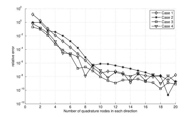
Figure 3.3: Convergence of tensor Gauss-Legendre quadrature for integrals of type (3.10) for the cases 1-4.

3.3 Computation of the $H^{-1/2,-1/2}(\mathbb{S}^{2}\times[0,T])$-norm

In Section 5 we perform numerical experiments for a spherical scatterer, i.e. $\Gamma=\mathbb{S}^{2}$, and special right-hand sides of the form $g(x,t)=g(t)Y_{n}^{m},t\in[0,T]$, where $Y_{n}^{m}$ are the spherical harmonics of degree $n$ and order $m$. In this case the exact solution of the scattering problem also decouples in space and time and is of the form

$$\phi_{\text{exact}}(x,t)=\phi_{\text{exact}}(t)Y_{n}^{m}\quad\text{with}\quad(x,t)\in\mathbb{S}^{2}\times[0,T].$$

Explicit representations of these exact solutions were derived in [17] and will be used as reference solutions to test the numerical algorithm. In order to estimate the error of the Galerkin approximation $\phi_{\text{Galerkin}}$ a computation of the $H^{-1/2,-1/2}(\mathbb{S}^{2}\times[0,T])$-norm is necessary. Since this norm is difficult to compute directly we use the sesquilinear form (2.4) with its coercivity property (2.5) in order to obtain an upper bound for this norm (up to a constant).
In this article we consider only boundary element meshes consisting of flat triangles whose union defines a polyhedral surface approximation $\Gamma_{h}$ of the original surface $\Gamma$. Hence, the exact Galerkin solution is perturbed due to this surface approximation and we denote the sesquilinear form on $\Gamma_{h}$ by $a_{h}\left(\cdot,\cdot\right)$. In order to compare the exact solution with the Galerkin solution we will project the exact solution $\phi_{\operatorname*{exact}}$ to the approximate surface $\Gamma_{h}$ resulting in a function $\phi_{\text{exact}}^{h}$ on $\Gamma_{h}$. To measure the difference $\phi_{\operatorname*{exact}}^{h}-\phi_{\operatorname*{Galerkin}}$ in an approximated (squared) energy norm we plug it into the sesquilinear form $a_{h}(\cdot,\cdot)$. Let us assume as before that the Galerkin solution is defined on $\Gamma_{h}$ and that

$$\phi_{\text{Galerkin}}(x,t)\in V_{\text{Galerkin}}:=\text{span}\left\{b_{i}(t)\varphi_{j}(x),1\leq i\leq L,1\leq j\leq M\right\}.$$

Since in Section 5 we will mainly focus on the properties of the temporal discretization we introduce a discrete space on a fine time grid (using possibly higher order basis functions in time) which uses the same basis functions in space as $V_{\text{Galerkin}}$:

$$V_{\text{Galerkin}}^{\text{fine}}:=\text{span}\left\{\tilde{b}_{i}(t)\varphi_{j}(x),1\leq i\leq\tilde{L},1\leq j\leq M\right\}\subset H^{-1/2,-1/2}(\Gamma_{h}\times[0,T]).$$

We now approximate $\phi_{\text{exact}}$ and $\phi_{\text{Galerkin}}$ with functions $\phi_{\text{exact}}^{h,\tilde{L}},\phi_{\operatorname{Galerkin}}^{\tilde{L}}\in V_{\text{Galerkin}}^{\text{fine}}$ in order to efficiently evaluate the associated sesquilinear form.

For the spatial approximation of $\phi_{\text{exact}}$ we note that in the case of piecewise constant basis functions in space every $\varphi_{j},1\leq j\leq M$ is associated with a triangle $\Delta_{j}=\text{conv}\left\{A_{j},B_{j},C_{j}\right\}$, where $A_{j},B_{j},C_{j}\in\Gamma$. An approximation of $\phi_{\text{exact}}$ defined on $\Gamma_{h}\times[0,T]$ is then defined by

$$\phi_{\text{exact}}^{h}(x,t):=\phi_{\text{exact}}(t)\sum_{j=1}^{M}c_{j}^{h}\varphi_{j}(x),\quad\text{with}\quad c_{j}^{h}=Y_{n}^{m}|_{D_{j}}\quad\text{where}\quad D_{j}=\frac{A_{j}+B_{j}+C_{j}}{\|A_{j}+B_{j}+C_{j}\|}.$$

In the case of piecewise linear basis functions in space every $\varphi_{j},1\leq j\leq M$, is associated with a node $C_{j}\in\Gamma$ of the spatial mesh. A suitable approximation of $\phi_{\text{exact}}$ defined on $\Gamma_{h}\times[0,T]$ is in this case defined by

$$\phi_{\text{exact}}^{h}(x,t):=\phi_{\text{exact}}(t)\sum_{j=1}^{M}c_{j}^{h}\varphi_{j}(x),\quad\text{with}\quad c_{j}=Y_{n}^{m}|_{C_{j}}.$$

In order to obtain an approximation of $\phi_{\text{exact}}^{h}(x,t)$ in the space $V_{\text{Galerkin}}^{\text{fine}}$ we further approximate the temporal part $\phi_{\text{exact}}(t)$ with its best $L_{2}$-approximation in $\text{span}\left\{\tilde{b}_{i},1\leq i\leq\tilde{L}\right\}$ on the fine time grid. This leads to

$$\phi_{\text{exact}}(x,t)\approx\phi_{\text{exact}}^{h,\tilde{L}}(x,t):=\sum_{i=1}^{\tilde{L}}\sum_{j=1}^{M}c_{i}^{\tilde{L}}c_{j}^{h}\varphi_{j}(x)\tilde{b}_{i}(t).$$

Finally, the function

$$\phi_{\operatorname{Galerkin}}(x,t)=\sum_{i=1}^{L}\sum_{j=1}^{M}\alpha_{i}^{j}\varphi_{j}(x)b_{i}(t)=\sum_{j=1}^{M}\varphi_{j}(x)\underbrace{\sum_{i=1}^{L}\alpha_{i}^{j}b_{i}(t)}_{\phi_{j}(t)}$$

has to be approximated with a function in $V_{\text{Galerkin}}^{\text{fine}}$. For this we approximate the function $\phi_{j}(t)$ for every $1\leq j\leq M$ again with its best $L_{2}$-approximation in $\text{span}\left\{\tilde{b}_{i},1\leq i\leq\tilde{L}\right\}$. This defines coefficients $\tilde{\alpha}_{i}^{j}$ such that

$$\phi_{\operatorname{Galerkin}}(x,t)\approx\sum_{i=1}^{\tilde{L}}\sum_{j=1}^{M}\tilde{\alpha}_{i}^{j}\varphi_{j}(x)\tilde{b}_{i}(t)=:\phi_{\operatorname{Galerkin}}^{\tilde{L}}(x,t).$$

In order to estimate the error of the Galerkin approximation we denote $\text{err}_{G}:=\|\phi_{\text{Galerkin}}^{\tilde{L}}-\phi_{\text{exact}}^{h,\tilde{L}}\|_{H^{-1/2,-1/2}(\Gamma_{h}\times[0,T])}$. Since

$$\phi_{\text{Galerkin}}^{\tilde{L}}-\phi_{\text{exact}}^{h,\tilde{L}}=\sum_{i=1}^{\tilde{L}}\sum_{j=1}^{M}(\tilde{\alpha}_{i}^{j}-c_{i}^{\tilde{L}}c_{j}^{h})\varphi_{j}(x)\tilde{b}_{i}(t),$$

the coercivity estimate (2.5) leads to

$$\text{err}_{G}^{2} \lesssim a(\phi_{\text{Galerkin}}^{\tilde{L}}-\phi_{\text{exact}}^{h,\tilde{L}},\phi_{\text{Galerkin}}^{\tilde{L}}-\phi_{\text{exact}}^{h,\tilde{L}})$$

$$=\sum_{i=1}^{\tilde{L}}\sum_{k=1}^{\tilde{L}}\sum_{j=1}^{M}\sum_{l=1}^{M}\int_{0}^{T}\int_{\Gamma}\int_{\Gamma}(\tilde{\alpha}_{i}^{j}-c_{i}^{\tilde{L}}c_{j}^{h})(\tilde{\alpha}_{k}^{l}-c_{k}^{\tilde{L}}c_{l}^{h})\frac{\dot{\tilde{b}}_{i}(t-\|x-y\|)\varphi_{j}(y)\tilde{b}_{k}(t)\varphi_{l}(x)}{4\pi\|x-y\|}d\Gamma_{y}d\Gamma_{x}dt$$

$$=\sum_{i=1}^{\tilde{L}}\sum_{k=1}^{\tilde{L}}\sum_{j=1}^{M}\sum_{l=1}^{M}(\tilde{\alpha}_{i}^{j}-c_{i}^{\tilde{L}}c_{j}^{h})\mathbf{\tilde{A}}_{k,i}(j,l)(\tilde{\alpha}_{k}^{l}-c_{k}^{\tilde{L}}c_{l}^{h})$$

$$=(\boldsymbol{\tilde{\alpha}}-\mathbf{c})^{\operatorname{T}}\underline{\underline{\mathbf{\tilde{A}}}}(\boldsymbol{\tilde{\alpha}}-\mathbf{c})$$

with

$$\boldsymbol{\tilde{\alpha}}=\left(\boldsymbol{\tilde{\alpha}}_{i}\right)_{i=1}^{\tilde{L}},\quad\text{where}\quad\boldsymbol{\tilde{\alpha}}_{i}(j)=\left(\tilde{\alpha}_{i}^{j}\right)_{j=1}^{\tilde{M}}$$

and in the same way

$$\mathbf{c}=\left(\boldsymbol{c}_{i}\right)_{i=1}^{\tilde{L}},\quad\text{where}\quad\mathbf{c}_{i}(j)=\left(c_{i}^{\Delta t}c_{j}^{h}\right)_{j=1}^{M}.$$

We therefore use the quantities

$$\text{err}(\phi_{\text{exact}},\phi_{\text{Galerkin}}):=\sqrt{(\boldsymbol{\tilde{\alpha}}-\mathbf{c})^{\operatorname{T}}\underline{\underline{\mathbf{\tilde{A}}}}(\boldsymbol{\tilde{\alpha}}-\mathbf{c})}$$ (3.11)

and

$$\text{err}_{\text{rel}}(\phi_{\text{exact}},\phi_{\text{Galerkin}}):=\sqrt{\frac{(\boldsymbol{\tilde{\alpha}}-\mathbf{c})^{\operatorname{T}}\underline{\underline{\mathbf{\tilde{A}}}}(\boldsymbol{\tilde{\alpha}}-\mathbf{c})}{\mathbf{c}^{\operatorname{T}}\underline{\underline{\mathbf{\tilde{A}}}}\mathbf{c}}}$$ (3.12)

as measures for the error of our Galerkin approximation.

Remark 3.3.

Since the space on which the sesquilinear form $a(\cdot,\cdot)$ is coercive differs from the space where it is continuous (cf. [8]) it is an open question if the error measure (3.11) is actually equivalent to the $H^{-1/2,-1/2}(\Gamma_{h}\times[0,T])$-norm or if it only represents an upper bound (up to a constant).

4 A Posteriori Error Estimation in Time

In this section we want to introduce a suitable a posteriori error estimator in time. Since in practice the solution of the boundary integral equation (2.3) might be rough (oscillatory or non-smooth) at certain times and rather smooth at other times it is in general not optimal to choose a fine time grid with constant step size everywhere on the time interval $[0,T]$ in order to resolve such a solution. Instead, a suitably chosen time grid that is adapted to the local irregularities of the solution with a lower number of variable time steps might be advantageous in this case and can lead to a more efficient scheme.
Since it is in general not known in advance where the solution is rough the numerical method should detect automatically where a local refinement of the time grid is necessary. This is done via the above mentioned a posteriori error estimator which computes local quantities $\left(\eta_{i}\right)_{i=1}^{L}$ that are associated with the local error of the Galerkin approximation. These quantities serve as refinement indicators in the adaptive scheme.
Note that the Galerkin discretization in time is not a time stepping method but has to be solved for the entire time mesh as a coupled system. The (localized) error estimator then indicates which time intervals should be marked for refinement (cf. Figure 4.1). Our numerical experiments indicate that, for problems in wave propagation, it is essential that an a posteriori error indicator examines all time steps in history instead of trying to determine within a time stepping method which interval in the history has to be refined and to set back the current time step to the relevant one in the history.

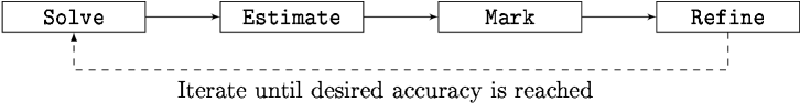
Figure 4.1: Adaptive strategy

The proposed algorithm currently uses the same time grid everywhere on the spatial domain in order to compute an approximation. Since the optimal time grid at different points of the scatterer might not coincide, we compute suitable refinements of the time grid at different points $x_{0}\in\Gamma$ and solve the scattering problem in the next step on the union of the proposed time grids. More precisely we perform the following steps in the time-adaptive algorithm:

Solve:

Solve the full problem (2.3) approximately for a given triangulation and time grid.

Estimate:

Choose a finite set of points $\Xi\subset\Gamma$ and compute, for each $x_{0}\in\Xi$, refinement indicators $\eta_{x_{0},i},1\leq i\leq L$, which are connected to the time step $t_{i}$ (also denoted as $t_{x_{0},i})$.

Mark:

Choose a threshold $\alpha\in(0,1)$ and mark for each $x_{0}\in\Xi$ all time steps $t_{x_{0},k}$ such that $\eta_{x_{0},k}\geq\alpha\max_{1\leq i\leq L}(\eta_{x_{0},i})$.

Refine:

For fixed $x_{0}\in\Xi$ insert additional timesteps in the middle of the subintervals $[t_{x_{0},k-1},t_{x_{0},k}]$ and $[t_{x_{0},k},t_{x_{0},k+1}]$, where $t_{x_{0},k}$ is a marked element. This leads to a refined time grid $\Delta_{x_{0}}$ for $x_{0}\in\Xi$. Choose $\Delta=\bigcup_{x_{0}\in\Xi}\Delta_{x_{0}}$ as the new time grid and iterate the procedure until a desired accuracy is achieved.

It remains to define suitable refinement indicators $\eta_{x_{0},i}$. Note that for the retarded single layer potential we have (see [8, Thm. 3])

$$S:H^{1,-1/2,-1/2}(\Gamma\times[0,T])\rightarrow H^{1/2,1/2}(\Gamma\times[0,T]),$$

where

$$H^{1,-1/2,-1/2}(\Gamma\times[0,T]):=\left\{\phi;\dot{\phi}\in H^{-1/2,-1/2}(\Gamma\times[0,T])\right\}$$

and

$$H^{1/2,1/2}\left(\Gamma\times\left[0,T\right]\right):=L^{2}\left(\left[0,T\right],H^{1/2}\left(\Gamma\right)\right)\cap H^{1/2}\left(\left[0,T\right],L^{2}\left(\Gamma\right)\right).$$

Remark 4.1.

Recall that in practical computations we solve the variational equation (2.4) approximately for $\dot{\phi}$ and obtain an approximate solution $\phi$ of the boundary integral equation in a postprocessing step. The refinement indicators that we will introduce are therefore based on the residual $S\dot{\phi}-\dot{g}$ which is in $H^{1/2,1/2}(\Gamma\times[0,T])$ due to the mapping properties of $S$. More precisely we have chosen the efficient and reliable a posteriori error estimator for operators of negative order that was originally developed for elliptic problems (see [4]) and adapted this estimator to the retarded potential integral equations.

The error estimators are based on an explicit representation of the $H^{1/2}$-seminorm. For an interval $\omega\subset\mathbb{R}$ it holds

$$|\xi|_{H^{1/2}(\omega)}^{2}=\int_{\omega}\int_{\omega}\frac{|\xi(t)-\xi(\tau)|^{2}}{|t-\tau|^{2}}d\tau dt.$$

For an arbitrary point $x_{0}\in\Xi$ on the boundary $\Gamma$ we define the residual

$$r_{x_{0}}(t):=S\dot{\phi}_{\text{Galerkin}}(x_{0},t)-\dot{g}(x_{0},t)$$

of the Galerkin approximation. Let a time grid as in (3.6) be given and define

$$\omega_{1}=[t_{0},t_{1}],\qquad\omega_{i}=[t_{i-2},t_{i}],\,2\leq i\leq l-1,\qquad\omega_{l}=[t_{l-2},t_{l-1}].$$

Then, local (temporal) refinement indicators are given by

$$\eta_{x_{0},i}:=|r_{x_{0}}|_{H^{1/2}(\omega_{i})}=\int_{\omega_{i}}\int_{\omega_{i}}\frac{|r_{x_{0}}(t)-r_{x_{0}}(\tau)|^{2}}{|t-\tau|^{2}}d\tau dt,\quad i=1,\ldots,l.$$ (4.1)

Due to the Lipschitz-continuity of the residual $r_{x_{0}}$, the integrand in (4.1) is non-singular. However, due to the removable singularity the double integral has to be evaluated with care. Here, we apply simple coordinate transformations which move the singularity to the boundary of the unit square and evaluate (4.1) using tensor-Gauss-Legendre quadrature rules. Let

$$\tilde{r}_{x_{0}}(t,\tau):=\frac{|r_{x_{0}}(t)-r_{x_{0}}(\tau+t)|^{2}}{|\tau|^{2}},\qquad\omega_{i}=[c,d]$$

and

$$\chi_{1}:t\mapsto(d-c)t+c,\qquad\chi_{2}:t\mapsto(d-c)t.$$

Then

$$|r_{x_{0}}|_{H^{1/2}(\omega_{i})} =\int_{\omega_{i}}\int_{\omega_{i}}\frac{|r_{x_{0}}(t)-r_{x_{0}}(\tau)|^{2}}{|t-\tau|^{2}}d\tau dt$$

$$=\int_{c}^{d}\int_{0}^{d-t}\tilde{r}_{x_{0}}(t,\tau)d\tau dt+\int_{c}^{d}\int_{c-t}^{0}\tilde{r}_{x_{0}}(t,\tau)d\tau dt$$

$$=\int_{c}^{d}\int_{0}^{t-c}\tilde{r}_{x_{0}}(-t+c+d,\tau)d\tau dt+\int_{c}^{d}\int_{0}^{t-c}\tilde{r}_{x_{0}}(t,-\tau)d\tau dt$$

$$=(d-c)^{2}\int_{0}^{1}\int_{0}^{t}\underbrace{\tilde{r}_{x_{0}}\left(-\chi_{1}(t)+c+d,\chi_{2}(\tau)\right)+\tilde{r}_{x_{0}}(\chi_{1}(t),-\chi_{2}(\tau))}_{=:\,\tilde{\tilde{r}}_{x_{0}}(t,\tau)}\,\,d\tau dt.$$

With the Duffy-transform $(t,\tau)\mapsto(t,t\tau)$ we map the triangle to the unit square and obtain

$$|r_{x_{0}}|_{H^{1/2}(\omega_{i})}=(d-c)^{2}\int_{0}^{1}\int_{0}^{1}\tilde{\tilde{r}}_{x_{0}}(t,t\tau)t\,\,d\tau dt.$$ (4.2)

The double integral in (4.2) can be approximated efficiently using tensor Gauss-Legendre quadrature since the integrand is well defined in the interior of the unit square.

5 Numerical Experiments

Convergence tests

In this section we present the results of numerical experiments. In order to test the convergence of the method we solve the boundary integral equation (2.3) for a spherical scatterer, i.e., $\Gamma=\mathbb{S}^{2}$ in the time interval $[0,1]$. In a first experiment we consider the purely time-dependent right-hand side

$$g(x,t)=t^{6}\operatorname{e}^{-4t},\quad(x,t)\in\mathbb{S}^{2}\times[0,1].$$ (5.1)

In this simple scenario the exact solution of the scattering problem is known explicitly (cf. [17, 18, 2]) and is given by

$$\phi(x,t)=2\partial_{t}g(x,t).$$ (5.2)

In a second experiment we consider the right-hand side

$$g(x,t)=g(t)Y_{1}^{0}:=t\sin(3t)^{2}\operatorname{e}^{-t}Y_{1}^{0},\quad(x,t)\in\mathbb{S}^{2}\times[0,1],$$ (5.3)

where $Y_{1}^{0}$ is a spherical harmonic of degree $1$ and order $0$. The exact solution of the problem is in this case given by

$$\phi(x,t)=\left[2\partial_{t}g(t)+2\int_{0}^{t}\sinh(\tau)\partial_{t}g(t-\tau)d\tau\right]Y_{1}^{0}.$$

For both configurations we discretize the scatterer using 2568 triangles and approximate the solution in space with piecewise linear basis functions, resulting in 1286 degrees of freedom in space.
The convergence of the method with respect to the stepsize $\Delta t$ is depicted in Figure 5.1 for different orders of the time discretization. The error was computed using the error measure from Section 3.3.

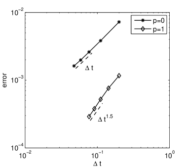
(a) $g(x,t)=t^{6}\operatorname{e}^{-4t}$

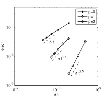
(b) $g(x,t)=t\sin(3t)^{2}\operatorname{e}^{-t}Y_{1}^{0}$

Figure 5.1: Convergence plots with respect to the stepsize in time.

Theoretical convergence rates of the Galerkin approach using piecewise polynomial basis functions were investigated in [1] for $p>0$. Since our PUM basis functions have the same approximation properties as the classical basis functions, the numerical experiments raise the important question whether these theoretical error bounds are sharp in general and the considered case of scattering from a sphere has special properties or, possibly, the discrete evaluation of the energy norm gains from, e.g., superconvergence properties . This will be a topic of future investigations.

Influence of the quadrature order

In Section 3.2 we showed that the entries of the boundary element matrix can be computed accurately with tensor Gauss quadrature rules. Here we want to test the influence of the quadrature order on the overall accuracy of the approximation. As an example we choose again a spherical scatterer that is discretized using 616 triangles. We consider the time interval $[0,5]$ which is subdivided into 20 equidistant subintervals. Note that the configuration was chosen such that the stepsize in time corresponds to the average diameter of the triangles. For the approximation we use piecewise linear basis functions in space and time (i.e. $p=1$). As right-hand side we choose a single Gaussian bump that travels in $x_{1}$ direction:

$$g(x,t)=\cos(t-x_{1})\operatorname{e}^{-6(t-x_{1}-5)^{2}},\quad x=(x_{1},x_{2},x_{3})^{\operatorname{T}}$$ (5.4)

In the following we compute the arising boundary element matrices with different accuracies. With $n_{\text{sing}},n_{\text{near}},n_{\text{far}}$ we denote the number of quadrature points that are used in each direction for the singular (regularized), the regular near field and the regular far field integrands, respectively (cf. [16]). As a reference solution we compute an approximation $\phi_{\text{high}}$ with $n_{\text{sing}}=20$, $n_{\text{near}}=15$ and $n_{\text{far}}=12$ on the same temporal and spatial grid mentioned above such that the discretization error is not visible. In Table 2 the results for different numbers of quadrature nodes are depicted. We measure the error between $\phi_{\text{high}}$ and the Galerkin solution using lower number of quadrature nodes in the error measure of Section 3.3 and in the $L^{2}([0,5],L^{2}(\Gamma))$-norm.

$n_{\text{sing}}$	$n_{\text{near}}$	$n_{\text{far}}$	$\text{err}_{\text{rel}}(\phi_{\text{high}},\phi_{\text{Galerkin}})$	rel. $L^{2}$-error
10	8	6	$1.86\cdot 10^{-6}$	$1.86\cdot 10^{-6}$
8	6	5	$1.43\cdot 10^{-5}$	$1.26\cdot 10^{-5}$
6	5	4	$1.03\cdot 10^{-4}$	$8.74\cdot 10^{-5}$
5	4	3	$5.36\cdot 10^{-4}$	$4.58\cdot 10^{-4}$
5	3	3	$1.43\cdot 10^{-3}$	$1.40\cdot 10^{-3}$
4	3	3	$1.87\cdot 10^{-3}$	$1.81\cdot 10^{-3}$
4	3	2	$2.48\cdot 10^{-3}$	$2.74\cdot 10^{-3}$

Table 2: Influence of quadrature on the accuracy of the Galerkin approximation

It becomes evident that a low number of quadrature nodes is sufficient to compute stable and reasonably accurate solutions. Note that the results obtained in Table 2 depend on the CFL number. Whereas a large CFL number is unproblematic with regard to the quadrature problem, a small CFL number, i.e. the step size in time is much smaller than the diameter of the triangles, typically requires a higher number of spatial quadrature nodes in order to obtain accurate solutions.

Long term stability

In order to test the stability of the method for a longer time interval we consider again a spherical scatterer and solve problem (2.3) for the right-hand side $g(x,t)=t^{4}\operatorname{e}^{-2t}$ for $T=40$. We discretize the time interval using 120 equidistant timesteps and local polynomial approximation spaces of degree $p=1$ resulting in 239 degrees of freedom in time. The sphere is discretized with 616 triangles, which leads to 310 degrees of freedom if piecewise linear approximation in space is used. The Galerkin solution at $x=(1,0,0)^{\text{T}}$ is depicted in Figure 5.2. We compare this result with the exact solution of the problem and with a numerical solution that is obtained using BDF2-convolution quadrature using also 120 time steps for the time discretization.

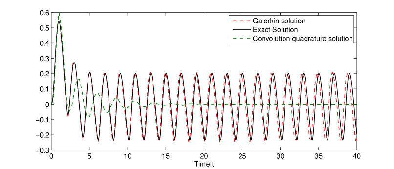
Figure 5.2: Galerkin and Convolution Quadrature solution compared to the exact solution of (2.3) for $\Gamma=\mathbb{S}^{2}$ and $g(x,t)=t^{4}\operatorname{e}^{-2t}$ in the time interval $[0,40]$.

It can be observed that the space-time Galerkin method leads to stable solutions also for long time computations. Due to the energy preservation of the method no numerical damping can be observed which is, e.g., typically the case for time discretizations schemes based on convolution quadrature (cf. Fig. 5.2). The slight shift of the numerical solution that is present in Figure 5.2 compared to the exact solution for large times is due to the insufficient approximation in space and furthermore due to the surface approximation of the sphere by flat triangles.

A non-convex scatterer

In Figure 5.3 we consider the scattering of a Gaussian pulse from a torus. We set the incoming wave as

$$u_{\text{inc}}(x,t):=8\cos(t-x_{1})\operatorname{e}^{-1.5(t-x_{1}-5)^{2}}\quad\text{for}\quad(x,t)\in\mathbb{R}^{3}\times[0,12]$$

and set the right hand side of the scattering problem (2.3) to

$$g(x,t)=-u_{\text{inc}}(x,t)\quad\text{for}\quad(x,t)\in\Gamma\times[0,12].$$

As illustrated in Figure 5.3 the incoming wave travels in $x_{1}$-direction towards the torus. We discretize the torus with 1152 flat triangles and use piecewise linear polynomials for the approximation in space. For the temporal discretization we use 100 equidistant timesteps in the interval [0,12] and approximate with local polynomial approximations spaces in time of degree 1.

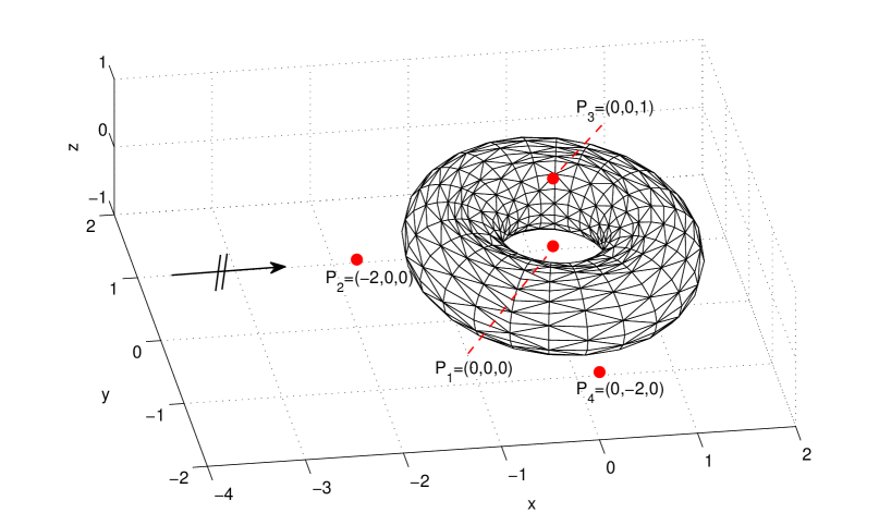
Figure 5.3: Scattering of a Gaussian pulse from a torus with observation points $P_{1},\cdots,P_{4}$.

We compute the scattered wave at four observation points $P_{1},\ldots,P_{4}$ in the exterior domain of the torus. The results are illustrated in Figure 5.4. As expected, the scattered wave at the points $P_{1}$ and $P_{3}$ exhibits small oscillations even after the incoming wave has passed. This is due to the non-convexity of scatterer and the associated waves that are trapped in the hole of the torus.

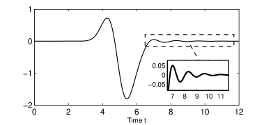
(a) Solution $u(x_{0},t)$ of the scattering problem at $x_{0}=P_{1}=(0,0,0).$

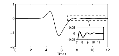
(b) Solution $u(x_{0},t)$ of the scattering problem at $x_{0}=P_{3}=(0,0,1).$

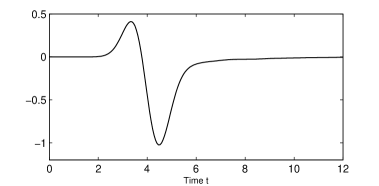
(c) Solution $u(x_{0},t)$ of the scattering problem at $x_{0}=P_{2}=(-2,0,0).$

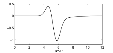
(d) Solution $u(x_{0},t)$ of the scattering problem at $x_{0}=P_{4}=(0,-2,0).$

Figure 5.4: Solutions of the scattering problem from the torus in Figure 5.3 for the points $P_{1},\cdots,P_{4}$ in the exterior domain.

Adaptivity in time

In this subsection we present numerical experiments that show the performance of the adaptive strategy described in Section 4. First we adopt again the setting of a spherical scatterer $\Gamma=\mathbb{S}^{2}$ and a right hand side of the form $g(x,t)=g(t)Y_{n}^{m}$. In this case the boundary integral equation (2.3) decouples and leads to the purely time-dependent problem: Find $\phi(t)$ such that

$$\int_{0}^{t}\mathcal{L}^{-1}(\lambda_{n})(\tau)\phi(t-\tau)d\tau=g(t),\,\,\,t\in[0,T],$$ (5.5)

where $\mathcal{L}^{-1}$ denotes the inverse Laplace transform and $\lambda_{n}(s)=I_{n+\frac{1}{2}}(s)K_{n+\frac{1}{2}}(s)$, where $I_{\kappa}$ and $K_{\kappa}$ are modified Bessel functions (cf. [18] for details). Note that $\phi(t)Y_{n}^{m}$, where $\phi(t)$ satisfies (5.5), is a solution of the full problem (2.3). It is convenient to observe the behavior of the time-adaptive scheme (i.e. the refinement process) using this one-dimensional problem since no spatial discretization takes place that might have an influence on the results. In the following we solve (5.5) by a Galerkin method for two different right-hand sides.
In a first experiment we set $n=0$ and consider $g(t)=t^{1.5}\operatorname{e}^{-t}$ on the time interval $[0,1]$. The exact solution of this problem is illustrated in Figure 5.5(a). Since the solution involves the first derivative of $g$ (cf. (5.2)) it is nonsmooth at $t=0$. For the numerical solution of this problem we use local polynomial approximation spaces of degree $p=1$ and use the error measure of Section 3.3. Figure 5.5(b) shows the error of the adaptive scheme compared to the approximation using equidistant time steps. Due to the nonsmoothness of the solution the equidistant approximation converges only with suboptimal rate. The adaptive algorithm converges significantly faster due to the successive refinement of the time grid towards the origin.
In the second experiment we again set $n=0$ and consider the right-hand side $g(t)=-\sin(10t)t^{3}\operatorname{e}^{-48(t-1)^{2}}$ on the time interval $[0,4]$. The exact solution of this problem is depicted in Figure 5.6(a). In this case the solution is smooth but oscillatory around $t=1$ and $t=3$. In Figure 5.7 different refinement levels of the adaptive approximation are shown. We start with a coarse time grid consisting of only 4 time steps and iterate the adaptive procedure ten times. It can be seen that at first the bump around $t=1$ is refined and only afterwards the refinement around $t=3$ begins. Intuitively this seems to be the right behavior since we solve a time-dependent wave propagation problem. Thus the solution at a later time can only be accurately resolved if the solution is already sufficiently approximated at earlier times. This behavior of the adaptive scheme repeats for higher refinement levels as indicated by the time grids at levels 8,9 and 10. The errors of the adaptive and the equidistant approximation are depicted in Figure 5.6(b).

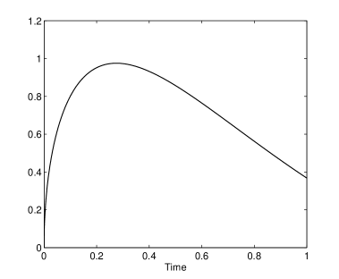
(a) Exact solution

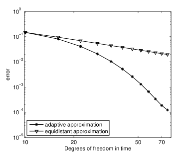
(b) Corresponding errors

Figure 5.5: Solution $\phi(t)$ of problem (5.5) for $g(t)=t^{1.5}\operatorname{e}^{-t}$ and the corresponding errors of the adaptive and the equidistant approximation.

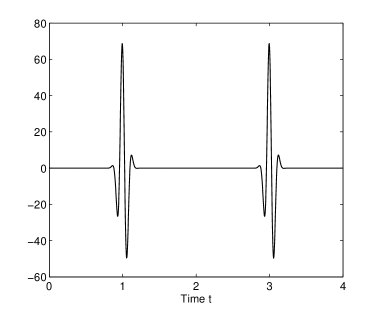
(a) Exact solution

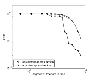
(b) Corresponding errors

Figure 5.6: Solution $\phi(t)$ of problem (5.5) for $g(t)=-\sin(10t)t^{3}\operatorname{e}^{-48(t-1)^{2}}$ and the corresponding errors of the adaptive and the equidistant approximation.

Figure 5.7: Different refinement levels

At last we test the adaptive algorithm for a full three-dimensional problem. We use a spherical scatterer discretized into 616 triangles and we set

$$g(x,t)=-H(t-x_{1}-2)\frac{(t-x_{1}-2)^{1.5}}{(t-x_{1}-2)^{2}+5}$$ (5.6)

for $x\in\mathbb{S}^{2}$ and $t\in[0,25]$. $H(\cdot)$ denotes the Heaviside step function. This right-hand side corresponds again to an incoming wave traveling in $x_{1}$-direction towards the scatterer which is met at $t=1$. Due to the low regularity of the right-hand side we expect also low regularity of the solution of the corresponding boundary integral equation. In Figure 5.8 two approximations of $\phi(x,t)$ at $(-1,0,0)^{\operatorname{T}}$ and $(1,0,0)^{\operatorname{T}}$ are illustrated . In both cases the approximations were computed using local polynomial approximation spaces of degree $p=1$ in time and piecewise linear functions in space. The solid lines represent the numerical solution that was obtained using the time-adaptive scheme. We started the adaptive algorithm with the coarse time grid $\{5\cdot l,l=0,\ldots,5\}$ and used the observation points $\Xi=\left\{(-1,0,0)^{\operatorname{T}},(0,1,0)^{\operatorname{T}},(1,0,0)^{\operatorname{T}}\right\}$ for the refinement indicators. The time grid after 6 iterations is shown in Figure 5.8. The dashed lines represent the numerical solution that was obtained using an equidistant time grid with the same number of timesteps.

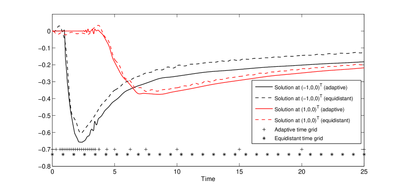
Figure 5.8: Comparison of the equidistant and adaptive approximation for problem (5.6).

The adaptive time grid is especially refined in the time interval $[1,3]$. The nonsmoothness of the solution in this interval is not surprising since the nonsmooth part of the incoming wave propagates through the obstacle at these times. Due to the refined time grid the adaptive solution at $(-1,0,0)^{\operatorname{T}}$ nicely captures the nonsmooth behavior of the solution in this time interval. The insufficient accuracy of the equidistant approximation in $[1,3]$ leads to a considerable shift of the numerical solution at later times that cannot be corrected with additional timesteps there. Similar observations can be made for the solution at $(1,0,0)^{\operatorname{T}}$.
Once the nonsmoothness of the right-hand side has passed the scatterer the solution seems considerably more smooth and large time steps are sufficient for an accurate approximation.

6 Conclusions

In this paper, we have introduced a fully discrete space-time Galerkin method for solving the retarded potential integral equations. The focus was on the efficient approximation of the integrals for building the system matrix, in particular, for $C^{\infty}$ temporal basis functions and combinations/convolutions thereof. It turned out that Gauss quadrature – in combination with regularizing coordinates for singular integrands – converges nearly as fast as for analytic functions in the accuracy regime of interest $\left[10^{-1},10^{-8}\right]$.

In addition we have introduced an a posteriori error estimator for retarded potential integral equations which is also employed for driving the adaptive refinement of the time mesh. Numerical experiments show that the resulting local error indicator captures very well local irregularities and oscillations in the solution and the resulting time meshes are much more efficient compared to uniform mesh refinement.
The adaptive refinement of the time mesh that we introduced in this paper is an important intermediate step towards a full space-time adaptive scheme. This will be an important further develpment in order to obtain a competitive method (see Remark 1.1).
Future work should furthermore address application to the Maxwell system and the theoretical analysis of the error estimator.

Acknowledgment. The second author gratefully acknowledges the support given by the Swiss National Science Foundation (No. P2ZHP2_148705).

References

- [1] A. Bamberger and T. H. Duong. Formulation Variationnelle Espace-Temps pur le Calcul par Potientiel Retardé de la Diffraction d’une Onde Acoustique. Math. Meth. in the Appl. Sci., 8:405–435, 1986.
- [2] L. Banjai and S. Sauter. Rapid solution of the wave equation in unbounded domains. SIAM Journal on Numerical Analysis, 47:227–249, 2008.
- [3] Y. Ding, A. Forestier, and T. H. Duong. A Galerkin scheme for the time domain integral equation of acoustic scattering from a hard surface. The Journal of the Acoustical Society of America, 86(4):1566–1572, 1989.
- [4] B. Faermann. Localization of the Aronszajn–Slobodeckij norm and application to adaptive boundary element methods: Part I. The two-dimensional case. IMA J. Num. Anal., 20:203–234, 2000.
- [5] B. Faermann. Localization of the Aronszajn-Slobodeckij norm and application to adaptive boundary element methods. Part II. The three-dimensional case. Numer. Math., 92(3):467–499, 2002.
- [6] M. Friedman and R. Shaw. Diffraction of Pulses by Cylindrical Obstacles of Arbitrary Cross Section. J. Appl. Mech., 29:40–46, 1962.
- [7] M. Gläfke. Adaptive Methods for Time Domain Boundary Integral Equations. PhD thesis, Brunel University, 2013.
- [8] T. Ha-Duong. On retarded potential boundary integral equations and their discretisation. In Topics in Computational Wave Propagation: Direct and Inverse Problems, volume 31 of Lect. Notes Comput. Sci. Eng., pages 301–336. Springer, Berlin, 2003.
- [9] T. Ha-Duong, B. Ludwig, and I. Terrasse. A Galerkin BEM for transient acoustic scattering by an absorbing obstacle. International Journal for Numerical Methods in Engineering, 57:1845–1882, 2003.
- [10] B. Khoromskij, S. Sauter, and A. Veit. Fast Quadrature Techniques for Retarded Potentials Based on TT/QTT Tensor Approximation. Computational Methods in Applied Mathematics, 11(3):342–362, 2011.
- [11] M. López-Fernández and S. A. Sauter. A Generalized Convolution Quadrature with Variable Time Stepping. Preprint 17-2011, Universität Zürich, accepted for publication in IMA J. Numer. Anal.
- [12] M. López-Fernández and S. A. Sauter. Generalized Convolution Quadrature with Variable Time Stepping. Part II: Algorithms and Numerical Results. Technical Report 09-2012, Institut für Mathematik, Universität Zürich, 2012.
- [13] C. Lubich. Convolution Quadrature and Discretized Operational Calculus I. Numerische Mathematik, 52:129–145, 1988.
- [14] J. Nédélec, T. Abboud, and J. Volakis. Stable solution of the retarded potential equations, Applied Computational Electromagnetics Society (ACES) Symposium Digest, 17th Annual Review of Progress, Monterey, 2001.
- [15] W. H. Press, S. A. Teukolsky, W. T. Vetterling, and B. P. Flannery. Numerical Recipes in C: The Art of Scientific Computing. Second Edition, 1992.
- [16] S. Sauter and C. Schwab. Boundary Element Methods. Springer Series in Computational Mathematics. Springer, 2010.
- [17] S. Sauter and A. Veit. Retarded Boundary Integral Equations on the Sphere: Exact and Numerical Solution. IMA Journal of Numerical Analysis, 2013, Online first: doi:10.1093/imanum/drs059.
- [18] S. Sauter and A. Veit. A Galerkin method for retarded boundary integral equations with smooth and compactly supported temporal basis functions. Numerische Mathematik, 123(1):145–176, 2013.
- [19] M. Schmid. Analysis of Tenor Gaussian Quadrature of Functions of Class . Master’s thesis, University of Zurich, 2013.
- [20] L. Trefethen. Is Gauss Quadrature Better than Clenshaw-Curtis? SIAM Rev., 50:67–87, February 2008.
- [21] D. S. Weile, G. Pisharody, N. W. Chen, B. Shanker, and E. Michielssen. A novel scheme for the solution of the time-domain integral equations of electromagnetics. IEEE Transactions on Antennas and Propagation, 52:283–295, 2004.