Non-self-similar blow-up in the heat flow for harmonic maps in higher dimensions

Abstract

We analyze the finite-time blow-up of solutions of the heat flow for $k$-corotational maps $\mathbb{R}^{d}\to S^{d}$. For each dimension $d>2+k(2+2\sqrt{2})$ we construct a countable family of blow-up solutions via a method of matched asymptotics by glueing a re-scaled harmonic map to the singular self-similar solution: the equatorial map. We find that the blow-up rates of the constructed solutions are closely related to the eigenvalues of the self-similar solution. In the case of $1$-corotational maps our solutions are stable and represent the generic blow-up.

Introduction

A map $F:M\to N\subset\mathbb{R}^{k}$ between two compact Riemannian manifolds $M$ and $N$ is called harmonic if it is a critical point of the functional

$$E(F)=\frac{1}{2}\int_{M}|\nabla F|^{2}\,dV_{M}.$$

The heat flow for harmonic maps was introduced by Eells and Sampson Eells and Sampson (1964) as a method of deforming any smooth map $F_{0}$ to a harmonic map via the equation

$$\partial_{t}F=(\Delta F)^{\top},\quad F|_{t=0}=F_{0},$$ (1)

where $(\Delta F)^{\top}$ is a projection of $(\Delta F)\in\mathbb{R}^{k}$ to $T_{F}N$—a tangent space to $N$ at the point $F$. For any solution to (1) we have

$$\frac{d}{dt}E(F)=-\int_{M}|\partial_{t}F|^{2}\,dV_{M}\leq 0.$$

If the flow exists for all times, $E(F)\geq 0$ converges to some $E_{\infty}$, suggesting that $F\to F_{\infty}$ with $F_{\infty}$ being a harmonic map. This approach proved to work only for target manifolds $N$ with non-positive sectional curvature. If there is a point in $N$ with positive sectional curvature, the gradient of a solution to (1) may blow-up in a finite time. In consequence, existence of global in time solutions may be established only in a weak sense Chen (1989). Moreover, the uniqueness of solutions can no longer be guaranteed Chen (1989). For explicit examples of non-unique weak solutions to (1) in the case of maps $\mathbb{R}^{d}\to S^{d}$ with $3\leq d\leq 6$ see Biernat and Bizoń (2011) and Germain and Rupflin (2011).

In order to overcome the problems posed by a finite-time blow-up and to investigate the circumstances in which the uniqueness is lost one has to fully understand the blow-up mechanism. The most general classification of solutions with a blow-up divides them into two types. We call a solution $F$ to (1) that blows up in finite time $T$ to be of type I if there exists a constant $C$ such that

$$(T-t)\sup_{M}|\nabla F|^{2}\leq C$$ (2)

holds for $t<T$ where $T$ is the blow-up time; if (2) does not hold the blow-up is of type II.

The reason for this classification becomes clear when we take maps $\mathbb{R}^{d}\to N$. Then, if the blow-up is of type I, we know that $F(x,t)=w\left(\frac{x-x_{0}}{\sqrt{T-t}}\right)$ near an isolated singularity located at $(x_{0},T)$ (Struwe, 1996, p. 293). The function $w:\mathbb{R}^{d}\to N$ describes the profile of a singular solution $F$ and the question of existence of singular solutions of type I reduces to the question of existence of admissible profile functions $w$. When the blow-up is of type II there is no similar universal description of what $F$ looks like near the singularity and any type II solution has to be considered on a case by case basis.

A careful reader will notice that $\mathbb{R}^{d}$ is not a compact manifold. Because in this paper we consider only isolated singularities it is a matter of convenience to replace the compact domain $M$ with a non-compact tangent space $T_{x_{0}}M=\mathbb{R}^{d}$, i.e. to neglect the curvature of the domain. Such simplification does not affect the blow-up mechanism.

Let us consider the simplest positively curved target, $S^{d}$ embedded in $\mathbb{R}^{d+1}$ in a canonical way. The deformation of a map $\mathbb{R}^{d}\to S^{d}$ according to the harmonic map heat flow (1) simplifies to

$$\partial_{t}F=\Delta F+|\nabla F|^{2}F.$$ (3)

Let us introduce spherical coordinates $(r,\omega)$ on $\mathbb{R}^{d}$ and coordinates $(u,\Omega)$ on $S^{d}$, with $u$ denoting the latitudinal position on $S^{d}$ and $\Omega\in S^{d-1}$ parametrizing the equator. Using these coordinates we can further restrict $F$ to a highly symmetric class of $k$-corotational maps

$$(r,\omega)\to(u(r,t),\Omega_{k}(\omega)).$$ (4)

$\Omega_{k}$ is a (non-constant) harmonic map with a constant energy density $\lvert\nabla\Omega_{k}\rvert^{2}=k(k+d-2)$, the number $k=1,2,3,\dots$ corresponds to a topological degree of map (4). The class of $k$-corotational maps is preserved by the harmonic map flow and the ansatz (4) reduces (3) to

$$\partial_{t}u=\frac{1}{r^{d-1}}\partial_{r}\left(r^{d-1}\partial_{r}u\right)-\frac{k(d+k-2)}{2r^{2}}\sin(2u).$$ (5)

The Dirichlet energy $E(F)$ can be expressed (up to a multiplicative constant) in terms of $u$ as

$$E(u)=\frac{1}{2}\int_{0}^{\infty}\left((\partial_{r}u)^{2}+k(d+k-2)\frac{\sin^{2}(u)}{r^{2}}\right)r^{d-1}\,dr$$ (6)

Regularity of $F$ enforces a boundary condition $u(0,t)=0$, while boundary condition at $r=\infty$ follows from the finiteness of Dirichlet energy $E(u)<\infty$. The monotonicity of energy

$$\frac{d}{dt}E(u)=-\int_{0}^{\infty}(\partial_{t}u)^{2}r^{d-1}\,dr\leq 0$$ (7)

ensures that the blow-up can happen only at $r=0$. Let us define $R(t)$ as the smallest spatial scale involved in the blow-up (obviously, $R(t)\to 0$ with $t\to T$). When we approach the blow-up time, the solution on the scale $r=\mathcal{O}(R(t))$ looks like $u(r,t)=Q\left(\frac{r}{R(t)}\right)$ for some fixed profile $Q$. This motivates the following definition of a blow-up rate

$$R(t)=\frac{1}{\sup_{r\geq 0}\,\lvert\partial_{r}u(r,t)\rvert}.$$ (8)

By the definition (8) of the blow-up rate $R(t)$, a re-scaled solution $u(r/R(t),t)$ has a bounded gradient for all times $t<T$:

$$\sup_{r\geq 0}\,\lvert\partial_{r}u(r/R(t),t)\rvert=1.$$

The blow-up mechanisms governed by (5) depend heavily on $k$ and $d$ and can be either Type I or Type II. For $k$-corotational maps in dimension $d=2$ van den Berg, Hulshof and King van den Berg et al. (2003) derived formal results for blow-up rates. In particular, for $1$-corotational maps, they conjectured that the generic blow-up is of Type II with the blow-up rate

$$R(t)\sim\frac{(T-t)}{|\log(T-t)|^{2}}\qquad\text{as }t\nearrow T.$$

Recently, this result has been proved by Raphael and Schweyer Raphaël and Schweyer (2013) by using methods coming from analysis of dispersive equations. For $1$-corotational maps in dimension $2$ other, non-generic blow-up rates, are also possible Angenent et al. (2009).

For $1$-corotational maps in dimensions $3\leq d\leq 6$ Fan Fan (1999) used ODE methods to prove the existence of a countable family $\{f_{n}\}_{n=1,2,\dots}$ of self-similar solutions for which

$$R(t)\sim(T-t)^{\frac{1}{2}}.$$

Later, Biernat and Bizoń Biernat and Bizoń (2011) showed, via numerical and analytical methods, that only $f_{1}$ is linearly stable and corresponds to a generic Type I blow-up. Gastel Gastel (2002) proved that the solution $f_{1}$ exists also for $k$-corotational maps as long as $3\leq d<2+k(2+2\sqrt{2})$. On the other hand, there are no results in the literature on dimensions $d>2+k(2+2\sqrt{2})$, even for $1$-corotational maps.

Statement of the main result

In our paper we use a method of matched asymptotics to construct a generic type II solution for $1$-corotational maps in dimensions $d\geq 7$. As $t\nearrow T$, the blow-up rates of these solutions are asymptotically given by

$$R(t) \sim\frac{C(T-t)^{\frac{1}{2}}}{-\log(T-t)-\kappa} \text{for }d =7$$ (9)

$$R(t) \sim\kappa(T-t)^{\frac{1}{2}+\beta_{1}} \text{for }d >7$$ (10)

with $\beta_{1}>0$ defined as

$$\beta_{1}=-\frac{1}{2}+\frac{2}{d-2-\omega},\quad\omega=\sqrt{d^{2}-8d+8}.$$ (11)

For each blow-up rate the constant $\kappa$ represents the dependence on initial data, while in (9) the constant $C$ is a fixed number. Interestingly, the blow-up rate in dimension $d=7$ is, to the leading order, equal to

$$R(t)=\frac{C(T-t)^{\frac{1}{2}}}{-\log(T-t)}(1+\mathcal{O}(\lvert\log(T-t)\rvert^{-1})),\qquad t\nearrow T$$

so, in dimension $7$, the blow-up rate is asymptotically independent of initial data.

Dimension $d=7$ can be seen as a borderline between type I and type II blow-ups. If one forgets about the underlying geometric setup and allows for non-integer values of $d$, then all our results remain valid. For $d$ slightly less than $7$ numerical evidence indicates a presence of a generic type I blow-up. On the other hand, when $d$ approaches $7$ from above, $\beta_{1}$ continuously drops to zero. So for $d<7$ we have a type I blow-up but for all $d>7$ we have a power-law type II blow-up of the form (10). Naively, one could arrive to a conclusion that for $d=7$ we should have a type I blow-up. Instead, we get a type II blow-up (9) corresponding to a type I blow-up rate with a logarithmic correction. The transition from type I to type II solution at $d=7$ also indicates that the self-similar solutions to (9) cease to exist for $d\geq 7$; but analysis of these vanishing self-similar solutions is beyond the scope of this paper.

In fact, the results for $1$-corotational maps are a special case of a more general result for $k$-corotational maps that we derive. For $k$-corotational maps with dimension $d$ and any positive integer $N$ satisfying

$$R_{N}(t) \sim\kappa(T-t)^{\frac{1}{2}+\beta_{N}} \text{for}\qquad\begin{split}d&>2+k(2+2\sqrt{2})\\ N&>\frac{1}{4}(d-2-\omega),\end{split}$$ (12)

$$R_{N}(t) =\frac{C\,(T-t)^{\frac{1}{2}}}{(-\log(T-t)+s_{0})^{\frac{1}{\delta}}} \text{for}\qquad\begin{split}d&>2+k(2+2\sqrt{2})\\ N&=\frac{1}{4}(d-2-\omega),\end{split}$$ (13)

with $\beta_{N}>0$ defined as

$$\beta_{N}=-\frac{1}{2}+\frac{2N}{d-2-\omega},\quad\omega=\sqrt{(d-2(k+1))^{2}-8k^{2}}$$

and $\delta>0$ equal to

$$\delta=\min(\omega,d-2-\omega).$$ (14)

From the dynamical system point of view, each of these solutions corresponds to a saddle point with $N-1$ unstable directions. The constants $\kappa$ and $s_{0}$ depend on initial data, while $C$ is a function of $d$ and $k$ only. This means that asymptotically blow-up rate (50) is universal for all initial data:

$$R_{N}(t)=\frac{C\,(T-t)^{\frac{1}{2}}}{(-\log(T-t))^{\frac{1}{\delta}}}(1+\mathcal{O}(\lvert\log(T-t)\rvert^{-1})),\qquad\text{as }t\nearrow T.$$

To obtain the blow-up rates we employed a technique, called matched asymptotics, which allows to construct approximate solutions to a differential equation on several spatial scales. The method of matched asymptotics expansions was also used to obtain formal type II solutions for the equation $\partial_{t}u=\Delta u+u^{p}$ in Herrero and Velázquez (1994) (see Herrero and Velázquez for details); these solutions have a similar stability properties as solutions (49). On the other hand, the case of $1$-corotational maps in $d=7$ (and (50) in general) resembles the solutions found by Herrero and Velázquez who used matched asymptotic to derive blow-up rates for chemotaxis aggregation in Herrero and Velázquez (1996); Velázquez (2002) and for the problem of melting ice balls in Herrero and Velázquez (1997).

As in the papers of Herrero and Velázquez, the blow-up rates are closely connected to the eigenvalues of a singular self-similar solution. In the case of $k$-equivariant harmonic maps, this singular solution is remarkably simple, as it corresponds to a singular equatorial map $u(r,t)=\frac{\pi}{2}$. The eigenvalues coming from linearization around the equatorial map ($\lambda_{N}=-\frac{d-2-\omega}{2}+N$ for $N=0,1,2,\dots$, see also (30)) relate to the blow-up rate exponents via $\beta_{N}=\frac{\lambda_{N}}{(d-2-\omega)}$. The interesting case of neutral eigenvalues, $\lambda_{N}=0$, requires us to include non-linear corrections into our analysis and gives rise to the logarithmic terms in the blow-up rate (50). Because there are two ways in which the nonlinear term can enter the equation, we have to estimate both of them and decide which is the dominant one. Surprisingly, this dominance—and thus the blow-up mechanism—is not set in stone but it depends on the dimension, which is reflected by a peculiar formula (14).

The formal solutions constructed in this paper are a first step towards the rigorous proof of existence of Type II blow-up for the equations of heat flow for $k$-corotational harmonic maps. The solutions presented here will be proved to exist in the upcoming paper by the author and Yukihiro Seki Biernat and Seki . The proof bases on topological methods similar to the ones used by Herrero and Velazquez in Herrero and Velázquez .

Construction of a blowing up solutions

Preliminaries

To describe blow-up at time $T$ it is convenient to introduce the self-similar variables

$$y=\frac{r}{\sqrt{T-t}},\quad s=-\log(T-t),\quad f(y,s)=u(r,t)$$ (15)

in which the original equation (5) takes the following form

$$\partial_{s}f=\partial_{yy}f+\left(\frac{d-1}{y}-\frac{y}{2}\right)\partial_{y}f-\frac{k(d+k-2)}{2y^{2}}\sin(2f)$$ (16)

The boundary condition $u(0,t)=0$ trivially carries over as $f(0,s)=0$.

Self-similar solutions are stationary points of the above equation, if they existm they fully capture the blow-up rate (i.e. the solution is regular for all $s$ including $s=\infty$). For $1$-corotational maps a countable family $\{f_{n}\}_{n=1,2,\dots}$ of self-similar solutions was proved to exist for $3\leq d\leq 6$ by Fan Fan (1999). Biernat&Bizoń Biernat and Bizoń (2011) demonstrated that only the first member of the family, $f_{1}$, is linearly stable. Numerical evidence suggests that for $d\geq 7$ these solutions are absent and therefore the Type I blow-up is no longer possible. For higher topological degrees the only rigorous result on existence of self-similar solutions, that authors are aware of, is the one by Gastel Gastel (2002) who proved the existence of the monotone self-similar solution $f_{1}$ in dimensions $d\leq 2+k(2+2\sqrt{2})$. Numerical evidence suggests, that for all $k\geq 1$ and $d\leq 2+k(2+2\sqrt{2})$ there exists a countable family of self-similar solutions $\{f_{n}\}_{n=1,2\dots}$.

On the other hand, in any dimension $d$ and for any topological degree $k$ (16) there exists a singular stationary solution, $f(y,s)=\pi/2$. This solution is singular because it violates the boundary conditions at $y=0$. Linear stability of this solution heavily depends on $d$ and $k$. For $k=1$ and dimension $d\geq 7$, $f(y,s)=\pi/2$ is linearly stable (up to a gauge mode corresponding to the shift of blow-up time $T$). For $k\geq 2$ and $d>2+k(2+2\sqrt{2})$, $f(y,s)=\pi/2$ looses some stability and becomes a saddle point with a finite number of unstable directions. As we shall see, this solution plays the key role in the dynamics of the blow-up.

Boundary layer

The singular solution $f(y,s)=\pi/2$ serves as a starting point for our construction of a Type II blow-up. The first step is to assume that the constructed solution converges to $\pi/2$. The convergence to $\pi/2$ has to be non-uniform because of the boundary condition at the origin $f(0,s)=0$. The non-uniform convergence can be realized by a boundary layer of size $\epsilon(s)$ near the origin, where a rapid transition from $f=0$ to $f=\pi/2$ occurs. This transition can be described by changing variables in (16) to

$$\xi=\frac{y}{\epsilon(s)},\quad U(\xi,s)=f(y,s),$$ (17)

where the dependent variable $U$ solves

$$\epsilon^{2}\partial_{s}U=\partial_{\xi\xi}U+\left(\frac{d-1}{\xi}+(2\epsilon\dot{\epsilon}-\epsilon^{2})\frac{\xi}{2}\right)\partial_{\xi}U-\frac{k(d+k-2)}{2\xi^{2}}\sin(2U),\quad U(0,s)=0.$$ (18)

We expect convergence to $\pi/2$, so the width of the boundary layer must tend to zero with time, hence $\epsilon(s)\to 0$ for $s\to\infty$. Additionally, we assume that the derivative of $\epsilon$ is bounded by $\epsilon$ for large $s$ i.e. $\dot{\epsilon}(s)=\mathcal{O}(\epsilon(s))$ as $s\to\infty$. Under these assumptions one can drop the quadratic terms in $\epsilon$ and $\dot{\epsilon}$ from equation (18). This leads to a solution $U(\xi,s)=U^{*}(\xi)$, where $U^{*}(\xi)$ solves an ordinary differential equation

$$\frac{d^{2}U^{*}}{d\xi^{2}}+\frac{d-1}{\xi}\frac{dU^{*}}{d\xi}-\frac{k(d+k-2)}{2\xi^{2}}\sin(2U^{*})=0$$ (19)

with boundary condition $U^{*}(0)=0$ inherited from (18). Any $U^{*}$ solving (19) is also a stationary point of (5), i.e. $U^{*}$ is a $k$-corotational harmonic map.

Equation (19) possesses a scaling symmetry $\xi\to\lambda\xi$ (with $\lambda>0$), which implies that any $U_{\lambda}(\xi,s)=U^{*}(\lambda\xi)$ is also an admissible approximate solution to (18). To get rid of this ambiguity, we first notice, that any regular solution to (19) behaves like $U^{*}(\xi)=a\xi^{k}+\mathcal{O}(\xi^{3k})$ near the origin with some real $a$. We can fix the scaling freedom by setting $a=1$, or equivalently by introducing an additional boundary condition

$$U^{*}(\xi)=\xi^{k}+\mathcal{O}(\xi^{3k})\qquad\text{as }\xi\to 0.$$ (20)

Equation (19) simplifies to an autonomous system if we use variables $x$ and $v$ defined as $\xi=e^{x}$ and $2U^{*}(\xi)=\pi+v(x)$

$$v^{\prime\prime}+(d-2)v^{\prime}+k(d+k-2)\sin(v)=0.$$ (21)

The boundary condition $U^{*}(\xi)=\xi^{k}+\mathcal{O}(\xi^{3k})$ implies $v(x)=-\pi+e^{kx}+\mathcal{O}(e^{3kx})$ when $x\to-\infty$. Because (21) is an autonomous equation we can deduce some global properties of $U^{*}$ by analyzing the phase diagram of $\eqref{eq:v}$.

The solution to (21) subject to these boundary conditions has a mechanical interpretation of a motion of a damped pendulum with $v$ being the angular position and $x$ corresponding to the time. The boundary conditions demand that the pendulum starts inverted, $v=-\pi$, at time $x=-\infty$ and swings out of this unstable position. The damping term forces the pendulum to reach the bottom, $v=0$, when $x=\infty$. In the phase plane spanned by $(v,v^{\prime})$, this trajectory is a heteroclinic orbit starting at the saddle point $(-\pi,0)$ and ending at $(0,0)$. To get the asymptotic behavior of $U^{*}$ at $\xi\to\infty$ it is enough to linearize (21) at the endpoint of the heteroclinic orbit, as shown in Figure 1.

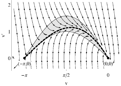
Figure 1: Phase diagram for the equation $0=v^{\prime\prime}+(d-2)v^{\prime}+k(d+k-2)\sin(v)$ with $k=1$ and $d=8$. A solution joining two critical points of the phase diagram is shown as a dashed line. Additionally, the plot depicts a trapping region $\mathcal{S}=\{(v,v^{\prime})\,|\,k\sin(v)\leq v^{\prime}\leq\gamma\sin(v)\}$, from which no solution can escape (here $\gamma=\frac{1}{2}(d-2-\sqrt{(d-2(k+1))^{2}-8k^{2}})=3-\sqrt{2}$). The trapping region $\mathcal{S}$ is used to prove estimates on a depicted solution in Theorem 1.

To analyze the asymptotic behavior of $v(x)$ for $x\to\infty$ we linearize the equation (21) at the stationary point $(0,0)$. The eigenvalues of the linearized equation are

$$\mu_{+}=-\gamma,\qquad\mu_{-}=-\gamma-\omega$$ (22)

with constants $\gamma=\frac{1}{2}(d-2-\omega)$ and $\omega=\sqrt{(d-2(k+1))^{2}-8k^{2}}$. From the form of the eigenvalues $\mu_{\pm}$ we see that the stationary point $(0,0)$ is a stable spiral for $d<d^{*}:=2+k(2+2\sqrt{2})$ but changes to a stable node when $d\geq d^{*}$. It follows that the asymptotic behavior of $v$, and consequently of $U^{*}$, can be either oscillatory or non oscillatory depending on $d$ for a given $k$. To proceed with our construction, we have to assume the latter—non oscillatory—behavior, that is $d\geq d^{*}$. For the particular case of $1$-corotational maps this condition simplifies to $d\geq 7$, if we consider only integer values of $d$.

There is one last thing to establish before we can make a claim about the asymptotic behavior of $U^{*}$. The formula for asymptotic behavior of $v$ near $(0,0)$, written explicitly, is

$$v(x)=2h_{+}\cdot e^{x\mu_{+}}(1+\mathcal{O}(e^{-2x}))+2h_{-}\cdot e^{x\mu_{-}}(1+\mathcal{O}(e^{-2x}))$$ (23)

(the factor of $2$ is a matter of convenience). Because $\mu_{+}>\mu_{-}$, the leading order term should be $2h_{+}e^{x\mu_{+}}$, unless $h_{+}$ is zero, in which case the dominant behavior changes to $2h_{-}e^{x\mu_{-}}$. In the appendix (Theorem 1) we exclude this possibility by proving that that $h_{+}$ is negative. We finally conclude that the asymptotic behavior of $U^{*}$ for large $\xi$ is

$$U^{*}(\xi)=\frac{\pi}{2}-h\xi^{-\gamma}(1+\mathcal{O}(\xi^{-2})+\mathcal{O}(\xi^{-\omega})),$$ (24)

with $h=-h_{+}>0$ depending only on $d$, and $\gamma>0$ defined as $-\mu_{+}$:

$$\gamma=\frac{1}{2}(d-2-\omega),\quad\omega=\sqrt{d^{2}-8d-8}.$$ (25)

Let us check where the approximation of $U(\xi,s)$ by $U^{*}(\xi)$ is valid. To arrive at the approximate equation (19) we had to drop the terms containing $\epsilon$ and $\dot{\epsilon}=\mathcal{O}(\epsilon)$. The approximation fails if one of the dropped terms becomes comparable with the remaining terms. For example we assumed that the remainder term in

$$\left(\frac{d-1}{\xi}+(2\epsilon\dot{\epsilon}-\epsilon^{2})\frac{\xi}{2}\right)=\frac{d-1}{\xi}(1+\mathcal{O}(\epsilon^{2}))$$

is small. But this assertion clearly fails for $\xi$ of order $1/\epsilon$, so the approximation $U(\xi,s)\approx U^{*}(\xi)$ can be valid only if $\xi\ll 1/\epsilon$ or, by definition (17), if $y\ll 1$.

Linearization around the singular solution

The boundary layer from the previous section resolves a conflict between the boundary condition $f(0,s)=0$ and the assumed convergence of $f(y,s)$ to $\pi/2$. In this section, we focus on describing the solution to (16) away from the boundary layer, i.e. for $y$ of order $1$. For such $y$, we expect the solution to stay close to $f=\pi/2$, so it is convenient to introduce a new variable $\psi$ defined as

$$f(y,s)=\pi/2+\psi(y,s).$$

The new variable $\psi$ solves

$$\partial_{s}\psi=-\mathcal{A}\psi+F(\psi),\qquad F(\psi)=\frac{k(d+k-2)}{2y^{2}}\left(\sin(2\psi)-2\psi\right)=\mathcal{O}(\psi^{3})$$ (26)

with operator $\mathcal{A}$ given by

$$-\mathcal{A}\psi=\frac{1}{\rho}\partial_{y}\left(\rho\partial_{y}\psi\right)+\frac{k(d+k-2)}{y^{2}}\psi,\quad\rho(y)=y^{d-1}e^{-y^{2}/4}.$$

A natural Hilbert space, arising in the context of operator $\mathcal{A}$ is

$$L^{2}(\mathbb{R}_{+},\rho\,dy)=\left\{f\in L^{2}_{loc}(\mathbb{R}_{+})\,\,|\,\,\int_{0}^{\infty}f(y)^{2}\rho(y)\,dy<\infty\right\}$$

with a canonical inner product

$$\langle f,g\rangle=\int_{0}^{\infty}f(y)g(y)\rho(y)\,dy.$$ (27)

It is routine to check that the operator $\mathcal{A}$, under the assumption $d>2+k(2+2\sqrt{2})$, is self-adjoint in $L^{2}(\mathbb{R}_{+},\rho\,dy)$ with domain $H^{1}(\mathbb{R}_{+},\rho\,dy)$ — a weighted Sobolev space defined in a canonical way.

To find the eigenfunctions of $\mathcal{A}$ we have to solve an ordinary differential equation

$$\frac{1}{\rho}\frac{d}{dy}\left(\rho\,\frac{d}{dy}\phi\right)+\frac{k(d+k-2)}{y^{2}}\phi=-\lambda\phi$$ (28)

with the condition $\phi\in H^{1}(\mathbb{R}_{+},\rho(y)\,dy)$. After a change of variables $\phi(y)=y^{-\gamma}w(y^{2}/4)$ and $z=y^{2}/4$ (with $\omega$ and $\gamma$ defined in (25)) equation (28) becomes

$$z\frac{d^{2}w}{dz^{2}}+\left(1-z+\frac{\omega}{2}\right)\frac{dw}{dz}=-\left(\lambda+\frac{\gamma}{2}\right)w.$$ (29)

with the condition $w\in H^{1}(\mathbb{R}_{+},e^{-z}z^{1+\omega/2}\,dz)$. Combination of the latter condition and the eigenvalue problem (29) leads to $w(z)=L^{(\omega/2)}_{n}(z)$ with $\lambda_{n}+\gamma/2=n$ ($n=0,1,2,\dots$), where $L^{(\alpha)}_{n}(z)$ denotes associated Laguerre polynomials. In terms of $\phi$ and $y$ these results read

$$\phi_{n}=\mathcal{N}_{n}y^{-\gamma}L_{n}^{(\omega/2)}(y^{2}/4),\quad\lambda_{n}=-\gamma/2+n,\quad n=0,1,2,\dots$$ (30)

The normalization constant

$$\mathcal{N}_{n}=2^{-1-\omega/2}\sqrt{\frac{\Gamma(n+1)}{\Gamma(n+1+\omega/2)}}$$ (31)

assures the orthonormality condition $\langle\phi_{n},\phi_{m}\rangle=\delta_{n,m}$. For completeness we shall add that the behavior of $\phi_{n}$ near the origin is

$$\phi_{n}=c_{n}y^{-\gamma}(1+\mathcal{O}(y^{-2})),\quad c_{n}=\frac{2^{-1-\omega/2}}{\Gamma(1+\omega/2)}\sqrt{\frac{\Gamma(1+n+\omega/2)}{\Gamma(1+n)}}.$$ (32)

Given the orthogonality relation and completeness of $\phi_{n}$ we can represent any solution to (26) as the following series

$$\psi(y,s)=\sum_{n=0}^{\infty}a_{n}(s)\phi_{n}(y),$$ (33)

In the above expression $a_{n}(s)$ solve non-linear equations

$$\dot{a}_{n}=-\lambda_{n}a_{n}+\langle F(\psi),\phi_{n}\rangle\quad\text{for }n=0,1,2,\dots$$ (34)

with $\dot{a}_{n}$ standing for the derivative of $a_{n}$ with respect to $s$ and $F(\psi)$ is defined in (26). Unfortunately, the presence of the non-linear coupling term $\langle F(\psi),\phi_{n}\rangle$ renders (34) impossible to solve in its current form. In the next section we will make assumptions on the form of $\psi$, that will allow us to estimate the non linear term. Consequently, we will be able to produce an approximate solution to (16).

Construction of a global solution

The analysis of the boundary layer solution gives us an approximation

$$f(y,s)\approx f_{inn}(y,s)=U^{*}\left(\frac{y}{\epsilon(s)}\right)\quad\text{for}\quad y\ll 1.$$ (35)

If we take $\epsilon\ll y\ll 1$ we can use the asymptotic formula (24) for $U^{*}$ to get

$$f_{inn}(y,s)=\frac{\pi}{2}-h\epsilon(s)^{\gamma}y^{-\gamma}$$ (36)

to the leading order. Because $\epsilon(s)\to 0$ with $s\to\infty$, the inner solution $f_{inn}(y,s)$ can get arbitrarily close to $\pi/2$ for a fixed $y$. But if $f(y,s)$ is close to $\pi/2$ the eigenfunctions of the linear operator $\mathcal{A}$ should work as a good approximation to the solution $f(y,s)$, so we write

$$f(y,s)\approx f_{out}(y,s)=\frac{\pi}{2}+\sum_{n=0}^{\infty}a_{n}(s)\phi_{n}(y)\quad\text{for}\quad y\gg\epsilon(s).$$ (37)

Without further assumptions, equations (34) for the coefficients $a_{n}$ cannot be solved. To proceed with our construction we have to reduce the number of independent degrees of freedom; we achieve this by assuming that one coefficient, say $a_{N}$, dominates the others, i.e.

$$\lvert a_{N}(s)\rvert\gg\lvert a_{n}(s)\rvert\qquad\text{for }n\neq N,\quad\text{and}\quad s\to\infty.$$ (38)

By (38) the outer solution is dominated by only one eigenfunction $\phi_{N}$ for large $s$

$$f(y,s)\approx f_{out}(y,s)=\frac{\pi}{2}+a_{N}(s)\phi_{N}(y)\quad\text{for}\quad y\gg\epsilon(s).$$ (39)

So far, this is the most arbitrary assumption we make, so it is critical to ensure that it does not lead to a contradiction at the end of the construction. In one of the following sections we verify this assumption and show which conditions on initial data does (38) require. This analysis leads to conclusions regarding the stability of constructed solutions.

Both approximations $f_{inn}$ and $f_{out}$ are compatible in the region $\epsilon\ll y\ll 1$ if we impose a relation between $a_{N}(s)$ and $\epsilon(s)$. Indeed, the outer solution behaves like

$$f_{out}(y,s)=\frac{\pi}{2}+a_{N}(s)\phi_{N}(y)=\frac{\pi}{2}+c_{N}a_{N}(s)y^{-\gamma}(1+\mathcal{O}(y^{2})).$$ (40)

(cf. (32)) and by comparing (40) with (36) we can choose $\epsilon$ such that

$$c_{N}a_{N}(s)=-h\epsilon(s)^{\gamma}.$$ (41)

Equation (41) is called the matching condition and it serves as a link between the inner solution and the outer solution.

Given solutions (35) and (39), together with condition (41), we can construct a global approximate solution, which is valid for all $y$,

$$f_{N}(y,s)=\begin{cases}f_{\text{inn}}(y,s)=U^{*}\left(\frac{y}{\epsilon(s)}\right)&\text{ for }y\leq K\\ f_{\text{out}}(y,s)=\pi/2-\frac{h}{c_{N}}\epsilon(s)^{\gamma}\phi_{N}(y)&\text{ for }y>K\end{cases}$$ (42)

with $K$ chosen so that $\epsilon\ll K\ll 1$ (e.g. $K=\sqrt{\epsilon}$). For an example of $f_{N}$ see Figure 2.

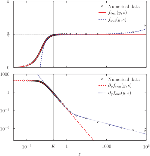
Figure 2: A snapshot at $s=13$ of a numerical solution $f(y,s)$ (in dimension $d=8$) compared to an approximation via inner and outer solutions combined into $f_{1}(y,s)$ (cf. definition (42)). The inner solution, $f_{inn}(y,s)$, is a good approximation for $y\ll 1$, while the outer solution, $f_{out}(y,s)$, is a good approximation when $f(y,s)$ is close to $\pi/2$. Both solutions coincide near a point $y=K=10^{-1}$.

At this point, we have an ansatz for a global solution with one unknown — function $\epsilon$. To get $\epsilon$ we have to go back to (34), with $n=N$ and $a_{N}(s)=-\epsilon(s)^{\gamma}\,h/c_{N}$ and solve

$$\gamma\dot{\epsilon}=-\lambda_{N}\epsilon-\,\frac{c_{N}}{h}\,\epsilon^{1-\gamma}\langle F(\psi),\phi_{N}\rangle\qquad\psi=f_{N}(y,s)-\pi/2.$$ (43)

The remaining question is in what way does the non-linear term $\langle F(\psi),\phi_{N}\rangle$ enter the equation? To answer this question we have to split $\langle F(\psi),\phi_{N}\rangle$ into contributions from inner and outer solutions. However, these computations are too technical for this section and would break the flow of the argument. Instead, we enclose the derivation in the next section and present the resulting formula here

$$\langle F(\psi),\phi_{N}\rangle=D_{N}\,\epsilon^{\gamma+\delta},\quad\delta=\min(\omega,2\gamma)>0,\quad D_{N}>0.$$ (44)

Combination of the estimate (44) and the equation (43) yields the following equation for $\epsilon$

$$\gamma\dot{\epsilon}=-\lambda_{N}\epsilon-\frac{D_{N}c_{N}}{h}\epsilon^{1+\delta}.$$ (45)

We can immediately discard negative eigenvalues $\lambda_{N}$, as they lead to $\epsilon$ which does not tend to zero; such $\epsilon$ violates our previous assumptions about the boundary layer.

The only viable solutions are those with $\lambda_{N}\geq 0$, which leads to two further cases. When $\lambda_{N}>0$ the non-linear term is of higher order and can be discarded for $s$ large enough leading to

$$\epsilon(s)=\epsilon_{0}\,e^{-\frac{\lambda_{N}}{\gamma}\,s}\qquad\text{for }\lambda_{N}>0$$ (46)

with $\epsilon(0)$ depending on initial data. On the other hand, when $\lambda_{N}=0$ the non-linear term becomes the leading order term resulting in

$$\epsilon(s)=\frac{C_{N}}{(s-s_{0})^{\frac{1}{\delta}}},\qquad C_{N}=\left(\frac{h\gamma}{c_{N}\,D_{N}\,\delta}\right)^{\frac{1}{\delta}}\qquad\text{for }\lambda_{N}=0.$$ (47)

We can now relate the blow-up rate $R(t)$ with $\epsilon$ via

$$R(t)=\frac{1}{\sup_{r\geq 0}\lvert\partial_{r}u(r,t)\rvert}=C_{s}\sqrt{T-t}\,\epsilon(s),\qquad C_{s}=\frac{1}{\sup_{\xi\geq 0}\lvert\frac{dU^{*}}{d\xi}(\xi)\rvert}.$$ (48)

If we combine (48), (46) and (47), and solve the conditions $\lambda_{N}>0$ and $\lambda_{N}=0$ for $N$ we get the following blow-up rates

$$R_{N}(t) =C_{s}\epsilon_{0}(T-t)^{\frac{1}{2}+\beta_{N}} \text{for}\qquad\begin{split}d&>2+k(2+2\sqrt{2})\\ N&>\frac{1}{4}(d-2-\omega)\end{split}$$ (49)

$$R_{N}(t) =\frac{C_{s}\,C_{N}(T-t)^{\frac{1}{2}}}{(-\log(T-t)-s_{0})^{\frac{1}{\delta}}} \text{for}\qquad\begin{split}d&>2+k(2+2\sqrt{2})\\ N&=\frac{1}{4}(d-2-\omega),\end{split}$$ (50)

with $\beta_{N}>0$

$$\beta_{N}=-\frac{1}{2}+\frac{2N}{d-2-\omega},\quad\omega=\sqrt{(d-2(k+1))^{2}-8k^{2}}$$ (51)

and $\delta>0$ being equal to

$$\delta=\min(\omega,d-2-\omega).$$ (52)

Approximation of the coupling term

According to the assumed form of the global solution $f_{N}(y,s)$ we can approximate the solution $\psi$ in the intervals $y\leq K$ and $y>K$ separately. Therefore, we split the integral $\langle F(\psi),\phi_{n}\rangle$ into

$$\langle F(\psi),\phi_{n}\rangle=\left(\int_{0}^{K}+\int_{K}^{\infty}\right)F(\psi)\phi_{n}(y)y^{d-1}e^{-y^{2}/4}\,dy=I_{inn}+I_{out}.$$

We compute the two integrals $I_{inn}$ and $I_{out}$ and compare them to see which one gives the leading order contribution. Our analysis leads to two qualitatively different approximations of the non-linear term

$$F(\psi)=\frac{k(d+k-2)}{2y^{2}}(\sin(2\psi)-2\psi)$$

depending on the choice of $d$ and $k$.

The first integral, $I_{inn}$, contains the contribution from the inner layer, where $\psi\approx f_{inn}-\pi/2$, so by (35) we can approximate $F(\psi)$ as

$$F(\psi)=F(f_{inn}(y,s)-\pi/2)=F(U^{*}(y/\epsilon)-\pi/2)=y^{-2}g(y/\epsilon),$$

for brevity we use a notation

$$g(\xi)=\frac{k(d+k-2)}{2}(\sin(2U^{*}(\xi)-\pi)-(2U^{*}(\xi)-\pi)).$$

When $y<K\ll 1$ we can replace the eigenfunction and the weight $\phi_{n}(y)\,y^{d-1}e^{-y^{2}/4}$ with its leading order term $\phi_{n}(y)\,y^{d-1}e^{-y^{2}/4}=c_{n}y^{-\gamma+d-1}(1+\mathcal{O}(y^{2}))$. We finally arrive at a simplified version of the integral $I_{inn}$

$$I_{inn}\approx c_{n}\int_{0}^{K}g(y/\epsilon)y^{d-3-\gamma}\,dy=c_{n}\epsilon^{d-2-\gamma}\int_{0}^{K/\epsilon}g(\xi)\xi^{d-3-\gamma}\,d\xi.$$ (53)

The upper bound $K/\epsilon$ in (53) tends to infinity as $s\to\infty$, so it is reasonable to check whether the integrand is divergent or convergent as $\xi\to\infty$. To this end we have to compute the asymptotic behavior of $g(\xi)$ at infinity. This can be done by using the asymptotic of $U^{*}$, as given by (24)

$$g(\xi)\approx-\frac{2k(d+k-2)}{3}(U^{*}(\xi)-\pi/2)^{3}\approx\frac{2k(d+k-2)h^{3}}{3}\xi^{-3\gamma}\quad\text{as }\xi\to\infty$$

The leading order of the integrand is thus $\xi^{d-3-4\gamma}$. By definitions (25) of $\gamma$ and $\omega$ there holds

$$d-2-\gamma=\gamma+\omega,$$ (54)

so the leading order term can be written as $\xi^{d-3-4\gamma}=\xi^{\omega-2\gamma-1}$.

We have to consider two cases, because the integral (53) can be divergent or convergent for large $(K/\epsilon)$ depending on the sign of $\omega-2\gamma$. If $\omega<2\gamma$, then the integral converges so, by taking the limit $K/\epsilon\to\infty$, we get

$$I_{inn}=\, c_{n}\epsilon^{d-2-\gamma}\int_{0}^{K/\epsilon}g(\xi)\xi^{d-3-\gamma}\,d\xi$$

$$=\, c_{n}\epsilon^{\gamma+\omega}\int_{0}^{\infty}g(\xi)\xi^{d-3-\gamma}\,d\xi.$$

But when $\omega>2\gamma$ the integral diverges as $(K/\epsilon)^{\omega-2\gamma}$, so we can replace the integral with its rate of divergence, in which case the lowest order approximation is

$$I_{inn}\approx\frac{2k(d+k-2)h^{3}c_{n}}{3}\epsilon^{\gamma+\omega}\left(\frac{K}{\epsilon}\right)^{\omega-2\gamma}=\frac{2k(d+k-2)h^{3}c_{n}}{3}\epsilon^{3\gamma}K^{\omega-2\gamma}.$$

We have to consider two similar cases when dealing with $I_{out}$. For $I_{out}$, $\psi$ is dominated by its approximation via a single eigenfunction $\psi=-\frac{h}{c_{N}}\epsilon^{\gamma}\phi_{N}$, which, together with $y>K$, results in $\lvert\psi\rvert\ll 1$ near the origin. So, as the first step to the approximation of $I_{out}$ we expand $F$ in a Taylor series around $\psi=0$

$$F(\psi)=F\left(-\frac{h}{c_{N}}\epsilon^{\gamma}\phi_{N}\right)\approx-\frac{k(d+k-2)}{y^{2}}\cdot\frac{3}{2}\left(-\frac{h}{c_{N}}\epsilon^{\gamma}\phi_{N}\right)^{3}=\frac{2k(d+k-2)h^{3}}{3y^{2}c_{N}^{3}}\epsilon^{-3\gamma}\phi_{N}^{3}.$$

If we use the Taylor expansion in $I_{out}$ we obtain

$$I_{out}=\frac{2k(d+k-2)h^{3}}{3c_{N}^{3}}\epsilon^{-3\gamma}\int_{K}^{\infty}\phi_{N}(y)^{3}\phi_{n}(y)y^{d-3}e^{-\frac{y^{2}}{4}}\,dy$$

which can be either divergent or convergent for small $K$. Near the origin ($y\to 0$) the leading order behavior of the integrand is

$$\phi_{N}(y)^{3}\phi_{n}(y)y^{d-3}e^{-\frac{y^{2}}{4}}=(c_{N})^{3}c_{n}\,y^{d-3-4\gamma}(1+\mathcal{O}(y^{2}))=(c_{N})^{3}c_{n}\,y^{\omega-2\gamma-1}(1+\mathcal{O}(y^{2})).$$

It is clear, that for $\omega<2\gamma$ the integral is finite and we can take the limit $K\to 0$, while for $\omega>2\gamma$ the integral is divergent and behaves like $(c_{N})^{3}c_{n}K^{\omega-2\gamma}$. These two cases can be expressed as

$$I_{out} \approx\frac{2}{3}k(d+k-2)h^{3}c_{n}\,\epsilon^{-3\gamma}\,K^{\omega-2\gamma}\quad \text{for }\omega<2\gamma,$$

and

$$\begin{split}I_{out}&\approx\,\epsilon^{-3\gamma}\,\frac{2k(d+k-2)h^{3}}{3c_{N}^{3}}\,\int_{0}^{\infty}\phi_{N}(y)^{3}\phi_{n}(y)y^{d-3}e^{-\frac{y^{2}}{4}}\,dy\\ &=\epsilon^{-3\gamma}\,T_{n}\end{split}\quad \text{for }\omega>2\gamma.$$

We are now in a position to compare the contributions from $I_{inn}$ and $I_{out}$

$$I_{inn} \propto\epsilon^{\gamma+\omega}, I_{out} \propto\epsilon^{\gamma+\omega}\,\left(\frac{\epsilon}{K}\right)^{2\gamma-\omega},\quad \text{for }\omega<2\gamma,$$

$$I_{inn} \propto\epsilon^{3\gamma}K^{\omega-2\gamma}, I_{out} \propto\epsilon^{3\gamma},\quad \text{for }\omega>2\gamma.$$

For sufficiently large times $I_{inn}$ dominates over $I_{out}$ when $\omega<2\gamma$ because the term $(\epsilon/K)^{2\gamma-\omega}$ tends to zero. On the other hand, when $\omega>2\gamma$ it is the other way around and $I_{out}$ dominates over $I_{inn}$ due to $K^{\omega-2\gamma}\to 0$. These two cases can be written in a unified way as

$$\langle F(\psi),\phi_{n}\rangle\approx D_{n}\epsilon^{\gamma+\delta},\quad\delta=\min(2\gamma,\omega).$$ (55)

with a constant

$$D_{n}=\begin{cases}c_{n}\int_{0}^{\infty}g(\xi)\xi^{d-3-\gamma}\,d\xi&\text{for }\omega<2\gamma\\ \frac{2(d-1)h^{3}}{3c_{N}^{3}}\,\int_{0}^{\infty}\phi_{N}(y)^{3}\phi_{n}(y)y^{d-3}e^{-\frac{y^{2}}{4}}\,dy&\text{for }\omega>2\gamma\,.\end{cases}$$

We intentionally avoided the case $\omega=2\gamma$, for which both integrals diverge logarithmically. This happens only for a non integer dimension $d=\frac{2}{3}\left(7+2\sqrt{7}\right)\approx 8.194\dots$, which we can exclude as incompatible with underlying geometric setting of the heat flow for harmonic maps.

One possible interpretation of this phenomenon-is a change of the way we should approximate the non-linear term $F(\psi)$ before the projection onto $\phi_{n}$. For example, when $\omega>2\gamma$, we can safely replace $F(\psi)$ with its Taylor expansion near $\psi=0$, i.e. $F(\psi)=\frac{2k(d+k-2)}{3y^{2}}\psi^{3}$. Projecting $F(\psi)$ back to $\phi_{n}$ gives negligible contribution from $I_{inn}$ and significantly larger contribution from $I_{out}$. At the same time, the value of $I_{out}$ is proportional to the third power of amplitude of $\psi\propto a_{N}$: $I_{out}\propto\epsilon^{3\gamma}\propto a_{N}^{3}$.

As for the other case, $\omega<2\gamma$, the contribution from the Taylor expansion is subdominant. Instead, a very small region $y<K$, of a diminishing size, governs the leading order behavior of non-linear term $F(\psi)$. We can replicate this effect by approximating $F(\psi)$ with a Dirac delta: $F(\psi)=G\epsilon^{\gamma+\omega}\delta(y)$. Indeed, to the leading order we get the same values for projections:

$$\langle F(\psi),\phi_{n}\rangle=G\epsilon^{\gamma+\omega}\langle\delta,\phi_{n}\rangle=Gc_{n}\epsilon^{\gamma+\omega}.$$

In fact, replacing the non-linear term $F(\psi)$ with a Dirac delta is the starting point to several derivations of Type II solutionsHerrero and Velázquez (1997, 1996). On the other hand, the Taylor expansion rarely shows up in derivations of the blow-up rate.

To verify whether $\langle F(\psi),\phi_{N}\rangle$ is positive (which is required for solution (47)) it suffices to show that $D_{N}>0$. The first case, when $D_{N}=c_{N}\int_{0}^{\infty}g(\xi)\xi^{d-3-\gamma}\,d\xi$ follows from the properties of the bounding region used in Theorem 1, which guarantees that $0\leq U^{*}(\xi)<\pi/2$, hence $g(\xi)>0$; combined with $c_{n}>0$ for every $n\geq 0$ we get the result. In the second case the result follows from the sign of the integrand in

$$\frac{2k(d+k-2)h^{3}}{3c_{N}^{3}}\,\epsilon^{-3\gamma}\int_{0}^{\infty}\phi_{N}(y)^{4}y^{d-3}e^{-\frac{y^{2}}{4}}\,dy>0.$$

and from $c_{N}>0$.

Note on stability of type II solutions

In this section we address two concerns that arose earlier in the text. The first one is an ex post validation of our assumption (38) about the dominance of $a_{N}$ over other coefficients $a_{n}$. The other issue is the stability of $f_{N}$. It appears that $f_{N}$ is unstable, because there is always a negative eigenvalue $\lambda_{0}=-\gamma/2$. To obtain any of the constructed solutions we will have to suppress this instability by fine tuning of initial data.

With an estimate on the non-linear term $\langle F(\psi),\phi_{n}\rangle$, we can actually solve equations (34) for $a_{n}$. By plugging (44) into (34) we get linear nonhomogeneous equations

$$\dot{a}_{n}=-\lambda_{n}a_{n}+D_{n}\epsilon^{\gamma+\delta},\qquad n\neq N$$

which can be explicitly solved by

$$a_{n}(s)=a_{n}(0)e^{-\lambda_{n}s}+D_{n}\int_{0}^{s}\epsilon(q)^{\gamma+\delta}e^{-\lambda_{n}(s-q)}dq.$$ (56)

The free parameters $a_{n}(0)$ are connected to initial data via

$$a_{n}(0)=\langle\psi,\phi_{n}\rangle|_{s=0}.$$ (57)

Let us start with the coefficients in front of higher eigenfunctions, i.e. $n>N$. It is enough to study the limit

$$\lim_{s\to\infty}\frac{a_{n}(s)}{a_{N}(s)}=-\frac{c_{N}}{h}\lim_{s\to\infty}\frac{a_{n}(0)+D_{n}\int_{0}^{s}\epsilon(q)^{\gamma+\delta}e^{\lambda_{n}\,q}\,dq}{e^{\lambda_{n}s}\epsilon(s)^{\gamma}}$$

The denominator diverges to infinity, while the numerator either diverges to $\pm\infty$ or converges to a constant. In the latter case the limit is $0$, and we are done. If the former is true, we apply l’Hôpital’s rule to get

$$\lim_{s\to\infty}\frac{a_{n}(s)}{a_{N}(s)}=-\frac{c_{N}\,D_{n}}{h}\lim_{s\to\infty}\frac{\epsilon(s)^{\delta}}{\gamma\dot{\epsilon}(s)/\epsilon(s)+\lambda_{n}}\underset{\text{Eq. }\eqref{eq:eps_final}}{=}-\frac{c_{N}\,D_{n}}{h}\lim_{s\to\infty}\frac{\epsilon(s)^{\delta}}{(\lambda_{n}-\lambda_{N})-D_{N}\,c_{N}\,\epsilon(s)^{\delta}/h}=0.$$

Hence, without any assumptions on $a_{n}(0)$ we have $\lvert a_{N}(s)\rvert\gg\lvert a_{n}(s)\rvert$ for $n>N$.

For $n<N$, let us rewrite (56) as

$$a_{n}(s)=\left(a_{n}(0)+D_{n}\int_{0}^{\infty}\epsilon(q)^{\gamma+\delta}e^{\lambda_{n}q}dq\right)e^{-\lambda_{n}s}-D_{n}\int_{s}^{\infty}\epsilon(q)^{\gamma+\delta}e^{-\lambda_{n}(s-q)}dq.$$ (58)

With elementary calculations and knowledge of $\epsilon$ one can show that the integrals in (58) converge if $n<N$. The second term in (58) is actually much smaller than $a_{N}(s)$. This is evident when we apply l’Hôpital’s rule to the limit

$$\lim_{s\to\infty}\frac{\int_{s}^{\infty}\epsilon(q)^{\gamma+\delta}e^{-\lambda_{n}(s-q)}dq}{a_{N}(s)} =\lim_{s\to\infty}\frac{\int_{s}^{\infty}\epsilon(q)^{\gamma+\delta}e^{\lambda_{n}q}dq}{e^{\lambda_{n}s}a_{N}(s)}\overset{\kern 2.0ptH}{=}\lim_{s\to\infty}\frac{-\epsilon(s)^{\gamma+\delta}}{\dot{a}_{N}(s)+\lambda_{n}a_{N}(s)}.$$

We continue with the help of matching condition $$c_{N}a_{N}(s)=-h\epsilon(s)^{\gamma} \epsilon$$ and equation (45) for to obtain

$$=-\frac{c_{N}}{h}\lim_{s\to\infty}\frac{\epsilon(s)^{\delta}}{(\lambda_{n}-\lambda_{N})-D_{N}c_{N}\epsilon(s)^{\delta}/h}=0.$$

In a similar way we can check that for $n<N$ the first term, containing $e^{-\lambda_{n}s}$, is actually much larger than $a_{N}(s)$. So if we want $\lvert a_{N}(s)\rvert\gg\lvert a_{n}(s)\rvert$ to hold, the coefficient in front of $e^{-\lambda_{n}s}$ in (58) has to be zero. This can be accomplished by selecting particular initial data for which

$$\langle\psi|_{s=0},\phi_{n}\rangle=a_{n}(0)=-D_{n}\int_{0}^{\infty}\epsilon(q)^{\gamma+\delta}e^{\lambda_{n}q}dq\qquad 0\leq n<N.$$ (59)

If the initial data, $\psi|_{s=0}$, fulfills the condition (59) the assumption $\lvert a_{N}(s)\rvert\gg\lvert a_{n}(s)\rvert$ does not lead to a contradiction.

The condition (59) for tthe solution $f_{N}$ imposes $N$ constraints on the initial data. Each constraint corresponds to one unstable direction along which our solution can diverge from the ansatz $f_{N}$. There is, however, one free parameter—the blow-up time $T$—that we can use to change the values of coefficients $a_{n}(0)$. Any small change $T\to T+\eta$ in blow-up time results in a small change of self-similar coordinates (15) $y\to y-\frac{1}{2}\eta e^{s}y+\mathcal{O}(e^{2s}\eta^{2})$ and $s\to s-\eta e^{s}+\mathcal{O}(e^{2s}\eta^{2})$. This change in self-similar coordinates affects the initial data $\psi|_{s=0}$ so the coefficients $a_{n}(0)$ also change. In particular, the zeroth coefficient becomes

$$a_{0}(0)\,\to\,a_{0}(0)-\eta\left\langle\partial_{s}\psi+\frac{y}{2}\partial_{y}\psi\,,\,\phi_{0}\right\rangle_{s=0}+\mathcal{O}(\eta^{2}).$$

It should be possible to choose a blow-up time $T$ in such way, that the new $a_{0}(0)$ fulfills the condition (59). This mechanism removes one of the constraints on initial data so $f_{N}$ has effectively $N-1$ unstable directions.

Discussion of the resultsy

In the previous section we analyzed the stability of $f_{N}$ concluding that the solution $f_{N}$ has $N-1$ unstable directions. On the other hand, $N$ is constrained by the condition $\lambda_{N}\geq 0$, or equivalently,

$$N\geq\frac{1}{4}(d-2-\omega)=\frac{1}{4}(d-2-\sqrt{(d-2(k+1))^{2}-8k^{2}})$$ (60)

with $d>2+k(2+2\sqrt{2})$. The right hand side of the inequality (60) depends on $k$ and $d$ and puts a lower bound on the possible $N$. In turn, the lower bound on $N$ induces a condition on the existence of stable $f_{N}$ for a given $k$. If we take arbitrary $k\geq 1$ and $d>2+k(2+2\sqrt{2})$ we can derive a lower bound on $N$

$$N\geq\frac{1}{4}(d-2-\omega)=\frac{1}{4}(d-2-\sqrt{(d-2(k+1))^{2}-8k^{2}})>\frac{k}{2},$$ (61)

so the instability of solutions $f_{N}$ increases with topological degree $k$.

Only a solution with $N=1$ can be stable, so from the bound $N>\frac{k}{2}$ we infer that for $k\geq 2$ there are no stable solutions $f_{N}$. Still, the solutions to (5) are guaranteed to blow up for large class of initial data. Numerical evidence suggests, that the generic blow-up is self-similar, so there has to exist at least one self-similar solution to (5) for $k\geq 2$. However, to the authors knowledge, in the literature there are no rigorous results concerning these solutions.

Because (61) is only a lower bound, one can ask if there are any examples of stable solutions. Stable solutions could exist only for $1$-corotational maps, so let us assume that $k=1$. The lower bound on $d$ then becomes $d>2+k(2+2\sqrt{2})=4+2\sqrt{2}\approx 6.828\dots$, but because dimension $d$ is an integer we arrive at $d\geq 7$. The first eigenvalue $\lambda_{1}=-\frac{\gamma}{2}+1$, which corresponds to the stable solution, is actually positive for all $d\geq 7$ so in this case there exists a stable solution $f_{1}$. In fact, numerical evidence suggests, that $f_{1}$ corresponds to a generic blow-up in dimensions $d\geq 7$.

Existence of a generic type I solution in a form of $f_{1}$ can be confirmed numerically, although solutions with finite-time singularities present several conceptual difficulties when solved on a computer. The most significant problem comes from the spatial resolution needed to resolve the shrinking scale of the boundary layer. We overcome this difficulty by employing a well established numerical method called a moving mesh, in which a constant number of mesh points is distributed dynamically to satisfy demands for high mesh density near the singularity, and outside of it. In particular, we modified Biernat an existing implementation Huang and Russell of moving mesh algorithm MOVCOL Russell et al. (2007). For an in-depth description of an application of MOVCOL to solutions with finite time singularity we refer the reader to a paper on a type II blow-up for chemotaxis aggregation by Budd et al.Budd et al. (2005).

For $d\geq 8$ the generic blow-up rate is given by

$$R(t)=C_{s}\epsilon_{0}(T-t)^{\frac{1}{2}+\beta_{1}},\qquad\beta_{1}=-\frac{1}{2}+\frac{2}{d-2-\omega},\qquad\omega=\sqrt{d^{2}-8d+8}.$$ (62)

By definition (8) $R(t)$ is inversely proportional to $\sup_{r\geq 0}\lvert\partial_{r}u(r,t)\rvert$, which can be easily obtained from numerical experiments. In fact, for $k=1$ the supremum is always attained at the point $r=0$, so we can replace $\sup_{r\geq 0}\lvert\partial_{r}u(r,t)\rvert$ with $\lvert\partial_{r}u(0,t)\rvert$. To verify the blow-up rate we study the ratio

$$\frac{\partial_{tr}u(0,t)}{\partial_{r}u(0,t)}=-\frac{R^{\prime}(t)}{R(t)},$$

which in $d\geq 8$ should tend to

$$\frac{\partial_{tr}u(0,t)}{\partial_{r}u(0,t)}\to\left(\frac{1}{2}+\beta_{1}\right)\qquad\text{as }t\nearrow T.$$

We compare $\beta_{1}$ obtained from numerical experiments with its theoretical value in Figure 3. An additional test compares the shape of a numerical solution near the origin with the shape of the function $f_{1}$ with its respective inner and outer solutions as in Figure 2. This plot captures a solution at time $T-t\approx 10^{-5.5}$.

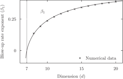
Figure 3: The predicted blow-up rate for $1$-corotational maps is $R(t)=(T-t)^{\frac{1}{2}+\beta_{1}}$ with $\beta_{1}=-\frac{1}{2}+\frac{2}{d-2-\omega}$ and $\omega=\sqrt{d^{2}-8d+8}$. The figure depicts the comparison between the predicted value of $\beta_{1}$ and $\beta_{1}$ obtained from numerical experiment via a relation $\frac{\partial_{tr}u(0,t)}{\partial_{r}u(0,t)}\to\left(\frac{1}{2}+\beta_{1}\right)$ with $t\nearrow T$. In each case the initial data was $u(r,0)=r$.

A more challenging numerical test is to verify the blow-up rate in dimension $d=7$. We expect (cf. equation (9)) the blow-up rate

$$R(t)=\frac{C\sqrt{T-t}}{(-\log(T-t)-s_{0})},\qquad C=\left(\frac{h\gamma}{c_{1}\,D_{1}}\right)\frac{1}{\sup_{\xi\geq 0}\lvert\frac{dU^{*}}{d\xi}(\xi)\rvert}.$$

This scenario is significantly more difficult to verify than (62) because in order to see the logarithmic correction we must get much closer to the blow-up time $T$. At the same time, the choice of initial data should only influence the constant $s_{0}$, but not $C$. We start with the relation $\partial_{r}u(0,t)=1/R(t)$, by which we get

$$\sqrt{T-t}\,\partial_{r}u(0,t)=C\,(-\log(T-t)-s_{0}).$$ (63)

To test our conjectured blow-up rate we plot the left hand side of (63) against $-\log(T-t)$, expecting to see a linear function after sufficiently long time. The experimental values of $C$, $T$ and $s_{0}$ are displayed in Table 1, while the relation (63) is depicted in Figure 4.

Acknowledgments

We thank Piotr Bizoń for the supervision of this paper. Special thanks are due to Juan L.L. Velázquez and Yukihiro Seki for very helpful discussions and suggestions. This work was supported by a Foundation for Polish Science IPP Programme “Geometry and Topology in Physical Models” and by the NCN Grant No. NN202 030740.

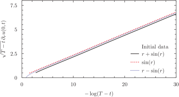
Figure 4: In dimension $d=7$, for a generic blow-up, the rate of blow-up is $R(t)=\frac{C(-\log(T-t)-s_{0}}{\sqrt{T-t}}$ with only $s_{0}$ depending on initial data. To verify that the blow-up rate agrees with numerical solution we study the quantity $\sqrt{T-t}R(t)$, which should be a linear function of $-\log(T-t)$ with slope independent on initial data. On the other hand, the shift $-C\,s_{0}$, should vary with initial data. In the picture we present results for initial data $u(r,0)=r$ and $u(r,0)=r\pm\sin(r)$, each with its own blow-up time $T$. The particular values of blow-up time, slope and shift are shown in table 1. The blow-up rate $R(t)$ is given by $\partial_{r}u(0,t)$.

Table 1: For $d=7$ it holds $\sqrt{T-t}\,\partial_{r}u(0,t)=C\,(-\log(T-t)-s_{0})$, asymptotically as $t\nearrow T$, with $C$ independent of initial data. In this table we compare values of $C$ and $s_{0}$ obtained from fitting the asymptotic relation to the numerical solution for various initial data. The values of $C$ indeed don’t change significantly among the tested initial data.

Initial data	T	$C$	$s_{0}$
$r$	$0.22913$	$0.22512$	$-0.43646$
$r+\sin(r)$	$0.066835$	$0.22475$	$0.45864$
$r-\sin(r)$	$0.44672$	$0.22500$	$-0.11921$

Appendix

Existence and asymptotic form of harmonic maps

Theorem 1.

For $d>2+k(2+2\sqrt{2})$, a solution $v(x)$ to equation

$$v^{\prime\prime}(x)+(d-2)v^{\prime}(x)+k(d+k-2)\sin(v)=0$$ (64)

subjected to boundary conditions

$$v(x)=-\pi+2e^{-kx}+\mathcal{O}(e^{-3kx}),\quad\text{for }x\to-\infty.$$

exists and has an asymptotic

$$v(x)=h_{+}\,e^{-\gamma x}(1+\mathcal{O}(e^{-2x})+\mathcal{O}(e^{-\omega x})),\quad\text{for }x\to+\infty$$

where $h_{+}$ is a strictly negative constant, while $\gamma$ and $\omega$ are defined in (25).

Proof. The proof bases on the analysis of a phase portrait spanned by $(v,v^{\prime})$ of autonomous equation (64) and consists of three steps.

Construction of no-escape region

Let us start by defining the vector field

$$F(v,v^{\prime})=(v^{\prime},-(d-2)v^{\prime}-k(d+k-2)\sin(v)).$$

We are interested in a heteroclinic orbit connecting two critical points of $F$, starting at $(-\pi,0)$ and ending at $(0,0)$. We construct a trapping region $\mathcal{S}=\{(v,v^{\prime})\,|\,-k\sin(v)\leq v^{\prime}\leq-\gamma\sin(v),-\pi<v<0\}$, which includes critical points $(-\pi,0)$ and $(0,0)$. No integral curve of $F$ starting in $\mathcal{S}$ can leave $\mathcal{S}$ (see Figure 1).

Indeed, if we define $\underline{n}(v)=(-k\cos(v),1)$ as a normal vector to a curve $v^{\prime}=-k\sin(v)$, pointing inward of $\mathcal{S}$, by a direct computation we get

$$F(v,-k\sin(v))\cdot\underline{n}(v) =-k^{2}\sin(v)(1-\cos(v))$$

which is positive for $-\pi<v<0$. Similarly, taking a normal vector $\overline{n}(v)=(-\gamma\cos(v),-1)$ (again directed inward $\mathcal{S}$) to a curve $v^{\prime}=-\gamma\sin(v)$ gives

$$F(v,-\gamma\sin(v))\cdot\overline{n}(v) =-\gamma^{2}\sin(v)(1-\cos(v))$$

which is also positive for $-\pi<v<0$. Therefore, the vector field $F$ points inward on the whole boundary of $\mathcal{S}$ (excluding the stationary points $(0,0)$ and $(-\pi,0)$). This implies that any integral curve of $F$ starting inside $\mathcal{S}$ must stay in $\mathcal{S}$.

Asymptotic of solutions starting in $\mathcal{S}$

There are two stationary points in $\mathcal{S}$ where a solution can end up. The first one, $(-\pi,0)$, can be ruled out because inside $\mathcal{S}$ vector field $F$ has a nonzero horizontal component pointing to the right. The remaining stationary point, $(0,0)$, gives a general asymptotic for of $v$ as

$$v(x)=2h_{+}\cdot e^{x\mu_{+}}(1+\mathcal{O}(e^{-2x}))+2h_{-}\cdot e^{x\mu_{-}}(1+\mathcal{O}(e^{-2x}))$$ (65)

where $\mu_{\pm}<0$ are eigenvalues of $\nabla F(0,0)$

$$\mu_{+}=-\gamma,\quad\mu_{-}=-\gamma-\omega.$$ (66)

At this point, $h_{-}$ and $h_{+}$ are constants depending on initial data and there are no restrictions on their values. Because $(v,v^{\prime})\in\mathcal{S}$, we have $v^{\prime}<-\gamma\sin(v)<-\gamma v$. If we combine the latter inequality with the asymptotic form of $v$, we get

$$-\omega h_{-}\cdot(1+\mathcal{O}(e^{-2x}))<0.$$ (67)

On the other hand, from $v<0$ we know that $h_{-}\cdot(1+\mathcal{O}(e^{-2x}))<0$. This contradicts with $\omega>0$, so $h_{+}\neq 0$. We can again use $v<0$, this time with leading order term proportional to $h_{+}$, to get $h_{+}<0$.

Boundary conditions in the thesis guarantee $(v,v^{\prime})\in\mathcal{S}$

When $x\to-\infty$ the solution $v$ with initial conditions $v(x)=-\pi+2e^{kx}+\mathcal{O}(e^{3kx})$ can be expanded as a Taylor series in $e^{x}$ in a following way

$$v(x)=-\pi+2e^{kx}-\frac{2(d+k-2)}{3(d+4k-2)}\,e^{3kx}+\mathcal{O}(e^{5kx})$$

It is a matter of routine computation to show that for sufficiently small $x$ we have

$$-k\sin(v(x))<v^{\prime}(x)<-\gamma\sin(v(x)).$$ (68)

So $(v,v^{\prime})\in\mathcal{S}$ and $v$ has an asymptotic form of (65) with $h_{+}<0$. $\square$

References

References

- Angenent et al. [2009] S. B. Angenent, J. Hulshof, and H. Matano. The Radius of Vanishing Bubbles in Equivariant Harmonic Map Flow from $D^2$ to $S^2$. SIAM Journal on Mathematical Analysis, 41(3):1121–1137, Jan. 2009. ISSN 0036-1410. doi: 10.1137/070706732.
- [2] P. Biernat. MOVCOL variation in Fortran 95. URL https://github.com/pwl/movcol.
- Biernat and Bizoń [2011] P. Biernat and P. Bizoń. Shrinkers, expanders, and the unique continuation beyond generic blowup in the heat flow for harmonic maps between spheres. Nonlinearity, 24(8):2211–2228, Aug. 2011. ISSN 0951-7715. doi: 10.1088/0951-7715/24/8/005.
- [4] P. Biernat and Y. Seki. Type II blow-up mechanisms in harmonic map heat flow, in preparation.
- Budd et al. [2005] C. J. Budd, R. Carretero-González, and R. D. Russell. Precise computations of chemotactic collapse using moving mesh methods. Journal of Computational Physics, 202(2):463–487, Jan. 2005. ISSN 00219991. doi: 10.1016/j.jcp.2004.07.010.
- Chen [1989] Y. Chen. The weak solutions to the evolution problems of harmonic maps. Mathematische Zeitschrift, 201(1):69–74, Mar. 1989. ISSN 0025-5874. doi: 10.1007/BF01161995.
- Eells and Sampson [1964] J. Eells and J. H. Sampson. Harmonic Mappings of Riemannian Manifolds. American Journal of Mathematics, 86(1):109, Jan. 1964. ISSN 00029327. doi: 10.2307/2373037.
- Fan [1999] H. Fan. Existence of the self-similar solutions in the heat flow of harmonic maps. Science in China Series A: Mathematics, 42(2):113–132, Feb. 1999. ISSN 1006-9283. doi: 10.1007/BF02876563.
- Gastel [2002] A. Gastel. Singularities of first kind in the harmonic map and Yang-Mills heat flows. Mathematische Zeitschrift, 242(1):47–62, Feb. 2002. ISSN 0025-5874. doi: 10.1007/s002090100306.
- Germain and Rupflin [2011] P. Germain and M. Rupflin. Selfsimilar expanders of the harmonic map flow. Annales de l’Institut Henri Poincare (C) Non Linear Analysis, 28(5):743–773, Sept. 2011. ISSN 02941449. doi: 10.1016/j.anihpc.2011.06.004.
- [11] M. Herrero and J. J. L. Velázquez. A blow-up result for semilinear heat equations in the supercritical case.
- Herrero and Velázquez [1994] M. Herrero and J. J. L. Velázquez. Blowup of solutions of supercritical semilinear parabolic equations. C. R. Acad. Sci. Paris Sér. I Math., 2(3):141–145, 1994. URL http://www.sciencedirect.com/science/journal/07644442.
- Herrero and Velázquez [1996] M. A. Herrero and J. J. L. Velázquez. Singularity patterns in a chemotaxis model. Mathematische Annalen, 306(1):583–623, Sept. 1996. ISSN 0025-5831. doi: 10.1007/BF01445268.
- Herrero and Velázquez [1997] M. A. Herrero and J. J. L. Velázquez. On the Melting of Ice Balls. SIAM Journal on Mathematical Analysis, 28(1):1–32, Jan. 1997. ISSN 0036-1410. doi: 10.1137/S0036141095282152.
- [15] W. Huang and R. D. Russell. MOVCOL webpage. URL http://www.math.ku.edu/~huang/research/movcol/movcol.html.
- Raphaël and Schweyer [2013] P. Raphaël and R. Schweyer. Stable Blowup Dynamics for the 1-Corotational Energy Critical Harmonic Heat Flow. Communications on Pure and Applied Mathematics, 66(3):414–480, Mar. 2013. ISSN 00103640. doi: 10.1002/cpa.21435.
- Russell et al. [2007] R. D. Russell, J. F. Williams, and X. Xu. MOVCOL4: A Moving Mesh Code for Fourth-Order Time-Dependent Partial Differential Equations. SIAM Journal on Scientific Computing, 29(1):197–220, Jan. 2007. ISSN 1064-8275. doi: 10.1137/050643167.
- Struwe [1996] M. Struwe. Geometric evolution problems. In Nonlinear Partial Differential Equations in Differential Geometry, pages 259—-339. IAS/Park City Mathematics Series, 1996.
- van den Berg et al. [2003] J. B. van den Berg, J. R. King, and J. Hulshof. Formal Asymptotics of Bubbling in the Harmonic Map Heat Flow. SIAM Journal on Applied Mathematics, 63(5):1682–1717, Jan. 2003. ISSN 0036-1399. doi: 10.1137/S0036139902408874.
- Velázquez [2002] J. J. L. Velázquez. Stability of Some Mechanisms of Chemotactic Aggregation. SIAM Journal on Applied Mathematics, 62(5):1581, 2002. doi: 10.1137/S0036139900380049.