Reconstructing the intermittent dynamics of the torque in wind turbines

Abstract

We apply a framework introduced in the late nineties to analyze load measurements in off-shore wind energy converters (WEC). The framework is borrowed from statistical physics and properly adapted to the analysis of multivariate data comprising wind velocity, power production and torque measurements, taken at one single WEC. In particular, we assume that wind statistics drives the fluctuations of the torque produced in the wind turbine and show how to extract an evolution equation of the Langevin type for the torque driven by the wind velocity. It is known that the intermittent nature of the atmosphere, i.e. of the wind field, is transferred to the power production of a wind energy converter and consequently to the shaft torque. We show that the derived stochastic differential equation quantifies the dynamical coupling of the measured fluctuating properties as well as it reproduces the intermittency observed in the data. Finally, we discuss our approach in the light of turbine monitoring, a particular important issue in off-shore wind farms.

1 Introduction

While wind energy can be taken as one of the best answers to the world-wide energetic problem[1], due to its particular physical features and turbulent nature it also presents challenging problems to be solved, even in more theoretical research fields such as physics and data analysis[2, 3]. One of such open problems is the ability for developing methods that reproduce the particular statistical properties shown in data series of power output or wind velocity measured at one wind turbine or wind energy converter (WEC). As it is known[2], since wind speed presents non-Gaussian fluctuations in time, the power output of one turbine shows also this intermittent behavior[4] making predictions of energy production rather difficult. Similarly, the intermittency of wind speed is also reflected in the torque of the shaft. Moreover, the loads applied by the wind on the WEC contribute significantly to determine the fatigue behavior and life expectancy of WECs[5, 6, 7]. Therefore, establishing good models for the intermittent evolution of the torque is an important task for better understanding and predicting the energy production and monitor the fatigue loads in WECs.

In this paper we focus on the fluctuations of the torque, assuming them as a direct result of atmospheric wind fields showing a high frequency of extreme events (non Gaussian). Recently, Milan et al[8] have conjectured that the anomalous wind statistics are responsible for the intermittent time evolution of the load, promoting additional fatigue of the turbine itself. Here we show that this is indeed the case, by deriving an evolution equation for the series of torque measurements that is constrained to the value of corresponding wind speeds. To this end we use and analyze measurements of wind, power and torque at one WEC of Alpha Ventus wind farm at the North Sea.

As we show below, initializing the differential evolution equation with the first values of our data series we are able to properly reproduce the time series of the torque as well as its main statistical features, including its intermittent behavior. Our approach follows from the method proposed in Ref. [4, 8] already applied to the power output of single WEC.

We start in Sec. 2 by describing the data analyzed and in Sec. 3 the method is described in further detail. Our results and comparative analysis is presented in Sec. 4 and conclusions and further discussions on this topic are given in Sec. 5.

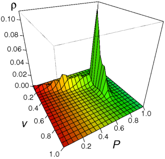
Figure 1: (Left) Location of the R04 WEC at the Alpha Ventus wind farm (red bullet) [Photo: Sean Gallup/Getty Images]. (Right) Joint probability density function as a function of the torque and of the wind velocity. All data was masked through normalization to the largest values (see text).

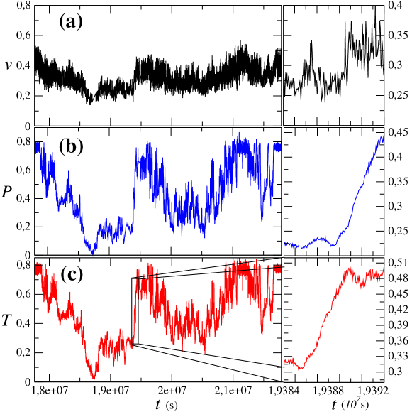
Figure 2: Sketch of time series of (a) the wind velocity $v$, (b) the power output $P$ and (c) the torque $T$. On the right a shorter time-interval of each series is plotted to illustrated a stronger fluctuation of power and torque. All data was masked through normalization to the largest values of $v$, $P$ and $T$ respectively.

2 Data: the Alpha Ventus off-shore wind farm

The data analyzed in this paper comprehends three sets of measurements, namely wind speed, power output and torque during the full month of January 2013. The data was measured at one WEC of the Alpha Ventus wind farm (see Fig. 1, left), also known as Borkum West. This wind farm is the first off-shore wind farm in Germany and it is located approximately at $54.3^{o}$N-$6.5^{o}$W. The torque is computed from the measurements of the power output $P$ and rotation number $n$, as $T=P/\omega$, with $\omega=n\pi/30$ the angular velocity of the operating shaft in units of rotations per minute. The selected WEC was AV04 from Senvion, formely RePower.

The sampling rate of the power output and torque is $50$ Hz and the sampling rate of the wind speed is $1$ Hz. Since we need to use the same sampling rate for all data series, we only consider power and torque measurements at instants for which a velocity measurement also exists ($1$ Hz).

All data series were analyzed according to all confidential protocols and were properly masked through the normalization by their highest values. Therefore the scientific conclusions are not affected by such data protection requirements.

The joint probability density function (PDF) $\rho(T,v)$ of both the wind speed and torque measurements is shown in Fig. 1 (right) and is according to the torque-velocity curve known in the literature[2, 9]. A time sampling of each data series is plotted in Fig. 2 (left) together with an example of one time period where both torque and power change abruptly (right). These abrupt fluctuations are the ones responsible for the intermittent behavior of the wind energy production and wind loads which can be easily seen in the increment statistics shown in Fig. 3.

To obtain the increment statistics of the torque $T$ we consider torque difference taken within a fixed time-gap $\tau$, namely

$$\Delta T_{\tau}(t)=T(t+\tau)-T(t),$$ (1)

and similarly for the wind speed and power output. As one sees from Fig. 3, for up to one hour or more, the increment distributions are clearly non-Gaussian, particularly the ones of torque and power. It is our purpose to provide a reconstruction procedure that reproduces the same intermittent statistics at several time scales, in order to better quantify the torque fluctuations.

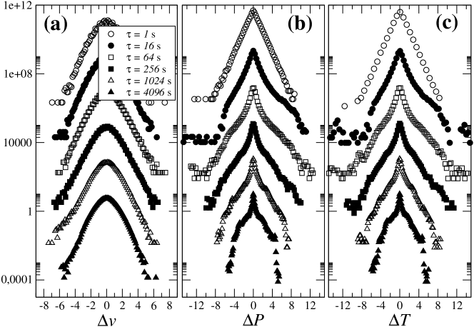
Figure 3: Probability density functions (PDFs) for the increments of (a) the wind velocity $\Delta v$, (b) the power output $\Delta P$ and (c) the torque $\Delta T$, for different time-lags $\tau$. The increments are plotted in units of the corresponding standard deviation (see text). The shift in the vertical axis is for better visualization.

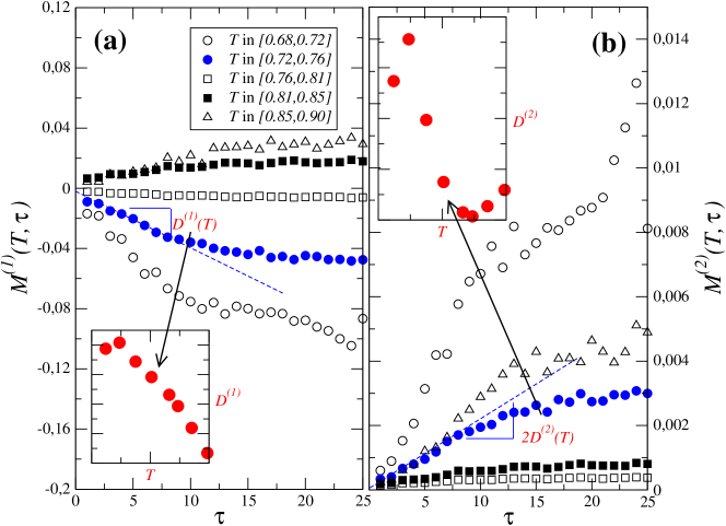
Figure 4: Conditional moments of the (a) first and (b) second order, for different values of the torque. In blue one illustrates the definition of the corresponding Kramers-Moyal coefficient, drift and diffusion, shown in the insets of (a) and (b) respectively.

3 Methodology: the conditioned Langevin approach

In 1997 a direct method to extract the evolution equation of stochastic series of measurements was proposed by Peinke and Friedrich[10]. Since then several applications of this framework were proposed and developed, ranging from turbulence modeling, to medical EEG monitoring and stock markets. For a review in this methods see Ref. [11] and references therein. The method was also applied in the context of wind energy, where it was shown its ability to properly define the power characteristic of single WECs[8, 12, 13].

The Langevin approach can briefly be described as follows. Assume we have a set of measurements $X(t)$ in time $t$ of one particular property $x$ evolving according to the stochastic equation

$$\frac{dx}{dt}=D^{(1)}(x)+\sqrt{D^{(2)}(x)}\Gamma_{t},$$ (2)

where $\Gamma_{t}$ is a Gaussian $\delta$-correlated white noise, i.e. $\langle\Gamma(t)\rangle=0$ and $\langle\Gamma(t)\Gamma(t^{\prime})\rangle=2\delta_{ij}\delta(t-t^{\prime})$. Equation (2) is usually called a Langevin equation[11]. With such an Ansatz, one separates the deterministic contribution to the evolution of $x$, given by the function $D^{(1)}$ (the drift), from the stochastic fluctuations incorporated by function $D^{(2)}$, called the diffusion. The constant in $\delta$-correlation and the square root in the Langevin equation are usually chosen for convenience.

By simple integration of the Langevin equation, one easily extracts a set of points similar to the sequence of, e.g., the torque measurements in Fig. 2(c). But the problem here is the inverse one: how can we arrive to a Langevin equation directly from the analysis of the set of measurements $X(t)$?

The answer has two main steps. The first one concerns to test if there is a time interval $t_{\ell}$ usually called the Markov length for which the succession of measurements are Markovian, i.e. the next value only depends on the present one and is independent of the values previous to it. Mathematically, to be Markovian means to fulfill the condition

$$\rho(X(t+t_{\ell})|X(t),X(t-t_{\ell}),X(t-2t_{\ell}),\dots)=\rho(X(t+t_{\ell})|X(t)),$$ (3)

with $\rho$ representing the conditional probability density functions that can be extracted from histograms of the data set. There are simple standard ways to perform this test[11]. When the measurements obey this Markov condition the next step can be carried out. However, in the case the Markov test fails, for instance in the presence of measurement noise[14], the next step can still be applied, after taking some cautions that we do not mention here. See Ref. [15] for details.

The second step, concerns the computation of both $D^{(1)}$ and $D^{(2)}$ that define Eq. (2), done through the corresponding conditional moments, illustrated in Fig. 4:

$$M^{(1)}(x,\tau) = \left\langle X(t+\tau)-X(t)|_{X(t)=x}\right\rangle$$ (4a)

$$M^{(2)}(x,\tau) = \left\langle(X(t+\tau)-X(t))^{2}|_{X(t)=x}\right\rangle$$ (4b)

where $\langle\cdot|_{X(t)=x}\rangle$ symbolizes a conditional averaging over the full measurement period.

Figure 4a and 4b shows the first and second conditional moments respectively, for different values of the torque, extracted from the data sets in Alpha Ventus. As one sees, for the lowest range of values of $\tau$, the conditional moments depend linearly on $\tau$. Since the two functions in Eq. (2) are, apart one multiplicative constant, the derivative of the two corresponding conditional moments with respect to $\tau$, namely

$$D^{(k)}(x)=\lim_{\tau\rightarrow 0}\frac{1}{k!}\frac{M^{(k)}(x,\tau)}{\tau}\quad,$$ (5)

with $k=1,2$ they can be directly extracted from the data sets. As illustrated in Fig. 4 with dashed lines, for each value $T$ both $D^{(1)}(T)$ and $D^{(2)}(T)$ are given by the slope of the linear interpolation of the corresponding conditional moments. Important additional insight can be taken from such plots. For instance, the linear fits of the conditional moments (dashed lines) for the lowest range of $\tau$-values typically cross the zero-axis. The absence of an offset for the conditional moments gives evidence of the absence of measurement noise[14, 15].

One important assumption however must be added: the set of measurements must be stationary. This is of course not the case of power and torque series. To overwhelm this shortcoming, Milan et al propose to consider a Langevin equation, but restricted to a sufficiently confined range of wind velocities[16]. Indeed, the statistical moments of the property being addressed are approximately constant if only a narrow range of wind velocities is considered. Such variant leads to what we call the conditioned Langevin equation:

$$\frac{dT}{dt}=D^{(1)}(T,v)+\sqrt{D^{(2)}(T,v)}\Gamma_{t},$$ (6)

where, for our purpose, $T$ represents the torque on the WEC and $v$ is the wind velocity.

4 Results: Reconstruction of the torque time series and statistics

Applying the methodology described in the previous section for ranges of wind velocity within $[\tilde{v},\tilde{v}+\Delta v]$ with $\Delta v=0.5$ and $\tilde{v}$ within the full range of observed values, we derive the numerical estimates of the drift $D^{(1)}$ and of the diffusion $D^{(2)}$ in Eq. (6).

Figures 5 (top) show the drift and diffusion coefficients respectively, each one as a function of the wind velocity and of the torque. While for low values of the velocity, $v\lesssim 0.3$, both coefficients are poorly defined, due to the lack of sampling, in the most sampled range $0.3\lesssim v\lesssim 0.7$ (check with Fig. 1) the drift and diffusion depend respectively linearly and quadratically on $T$. This dependence can be better seen in the two-dimensional plots of Fig. 5 (bottom).

Having extracted the functional dependence of both coefficients $D^{(1)}$ and $D^{(2)}$ we are now able to describe the evolution of the torque by keeping track of the wind velocity, simply through an Euler-like discrete version of the conditioned Langevin equation. We take the first measurement of both wind speed and torque as initial conditions for the stochastic equation and integrate it with respect to $t$ using at each integration step the observed wind velocity.

The reconstructed series are plotted in Fig. 6(a) together with the empirical series of torque measurements. Clearly, the reconstructed series are close to the real measurements. Moreover, the statistical distribution of the increments $\Delta T_{\tau}$ are also well reproduced for time scales from seconds up to hours (Fig. 6(b)). All in all, from Fig. 6, one can clearly conclude the ability for the conditioned Langevin model to properly describe the evolution of the torque in one WEC.

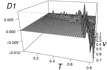
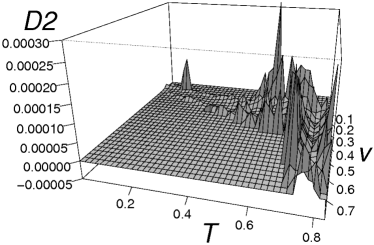
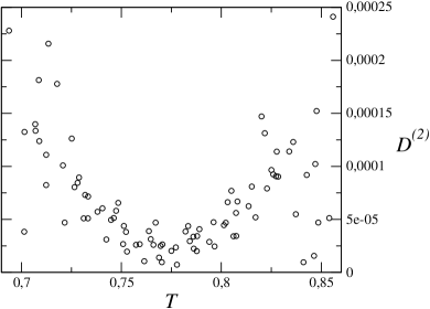
Figure 5: (Top) Numerical result for the drift $D^{(1)}(T,v)$ and diffusion $D^{(2)}(T,v)$ in the Langevin equation from which the time series of the torque is reconstructed. (Bottom) For the upper range of values of the wind velocity (around rated wind speed) one plots the projection of drift and diffusion on the $T$-axis. See text and Fig. 6.

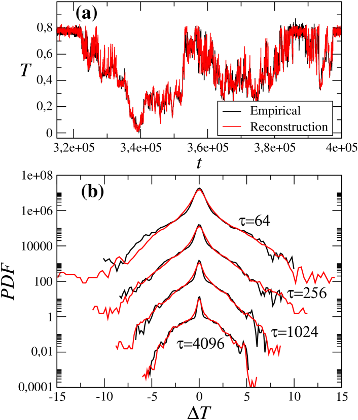
Figure 6: Reconstruction of the torque (in red) of torque measurements (black): (a) The explicit time-series of the torque and (b) the probability density function of the increments (fluctuations) of the torque within different time-lags. Time is in seconds, and the Torque increments is in units of corresponding standard deviations ($\sigma_{\tau}$).

5 Discussion and conclusions

In this paper we show how to reconstruct the series of torque measurements through a Langevin model conditioned to the wind velocity. The model reproduces well not only the series of torque measurements but also the intermittent feature of its increment statistics. It should be noticed that the validity of Eq. (6) is not fully guaranteed, since Pawula condition[17], $D^{(4)}=0$, was not tested. This condition is necessary for assuming a Langevin evolution equation. Still, even in the case Pawula theorem is not fulfilled, the conditioned Langevin equation can be taken as a first approximation of the stochastic evolution of the torque in one WEC.

The reproduction of torque time series of WECs here described is already significant, though the approximations used for the drift and diffusion coefficients are of first order only (see Fig. 4). Higher order approximations are possible and would improve the reproduction further[18, 19, 20, 21]. In these higher order corrections one considers the numerical values of the drift for the computation of the corresponding diffusion.

A critical remark should be stated at this point: while the model in Eq. (6) properly reproduces the stochastic evolution of the torque in WECs it depends on the wind velocity measurements. On one hand, nacelle anemometer wind velocity measurements are typically much less accurate than the measurements of other properties on the WEC, such as the pitch angle. On the other hand, being always coupled to a measured property, in this case the wind speed, the conditioned Langevin equation is not able to provide straightforward forecasts of loads even in the nearest time horizons.

Still, being able to properly describe the evolution of the torque, one can use it for providing additional input information for forecasting models, namely for training neural networks constructed for torque forecast.

Another important next step from this study is to ascertain if such an approach can be applied to other kinds of loads in WEC, namely bending moments. These points can contribute to improve monitoring protocols of WECs in off-shore wind farms and will be addressed in the near future as the next steps.

References

References

- [1] Johnson G 2006 Wind Energy Systems (Kansas State University)
- [2] Burton T, Sharpe D, Jenkins N and Bossanyi E 2001 Wind Energy Handbook (Wiley)
- [3] T Mücke D K and Peinke J 2011 Wind Energy 14 301–316
- [4] P Milan M W and Peinke J 2013 Phys. Rev. Lett. 110 138701
- [5] Ragan P and Manuel L 2007 Wind Engineering 31 83–99
- [6] Moriarty P 2008 Wind Energy 11 559–576
- [7] Freundenreich K and Argyriadis K 2008 Wind Energy 11 589–600
- [8] P Milan T Mücke D K and Peinke J 2013 Wind Energy in print
- [9] P Rinn M W and Peinke J 2013 Private communication
- [10] Friedrich R and Peinke J 1997 Phys. Rev. Lett. 78 863
- [11] Friedrich R, Peinke J, Sahimi M and Tabar M 2011 Phys. Rep. 506 87
- [12] E Anahua S Barth J P 2008 Wind Energy 11 219
- [13] Raischel F, Scholz T, Lopes V and Lind P 2013 Physical Review E 88 042146
- [14] FBoettcher, JPeinke, DKleinhans, RFriedrich, PGLind and MHaase 2006 Physical Review Letters 97 090603
- [15] PGLind, MHaase, FBoettcher, JPeinke, DKleinhans and Friedrich R 2010 Physical Review E 81 041125
- [16] P Milan M W and Peinke J 2013 Private communication
- [17] Risken H 1984 The Fokker-Planck Equation (Heidelberg: Springer)
- [18] Friedrich R, Siegert S, Peinke J, Lück S, Siefert M, Lindemann M, Raethjen J, Deuschl G and Pfister G 2000 Phys. Lett. A 271 217
- [19] Ragwitz M and Kantz H 2001 Phys. Rev. Lett. 87 254501
- [20] Friedrich R, Renner C, Siefert M and Peinke J 2002 Phys. Rev. Lett. 89 149401
- [21] Gottschall J and Peinke J 2008 New Journal of Physics 10 083034