Generalized Two-Qubit Whole and Half Hilbert-Schmidt Separability Probabilities

Abstract

Compelling evidence–though yet no formal proof–has been adduced that the probability that a generic (standard) two-qubit state ($\rho$) is separable/disentangled is $\frac{8}{33}$ (arXiv:1301.6617, arXiv:1109.2560, arXiv:0704.3723). Proceeding in related analytical frameworks, using a further determinantal $4F3$-hypergeometric moment formula (Appendix A), we reach, via density-approximation (inverse) procedures, the conclusion that one-half ($\frac{4}{33}$) of this probability arises when the determinantal inequality $|\rho^{PT}|>|\rho|$, where $PT$ denotes the partial transpose, is satisfied, and, the other half, when $|\rho|>|\rho^{PT}|$. These probabilities are taken with respect to the flat, Hilbert-Schmidt measure on the fifteen-dimensional convex set of $4\times 4$ density matrices. We find fully parallel bisection/equipartition results for the previously adduced, as well, two-“re[al]bit” and two“quater[nionic]bit” separability probabilities of $\frac{29}{64}$ and $\frac{26}{323}$, respectively. The new determinantal $4F3$-hypergeometric moment formula is, then, adjusted (Appendices B and C) to the boundary case of minimally degenerate states ($|\rho|=0$), and its consistency manifested–also using density-approximation–with an important theorem of Szarek, Bengtsson and Życzkowski (arXiv:quant-ph/0509008). This theorem states that the Hilbert-Schmidt separability probabilities of generic minimally degenerate two-qubit states are (again) one-half those of the corresponding generic nondegenerate states.

I Introduction

The problem of determining the probability that a bipartite/multipartite quantum state of a certain random nature exhibits a particular entanglement characteristic is clearly of intrinsic “philosophical, practical, physical” Życzkowski et al. (1998)) interest Życzkowski et al. (1998); Singh et al. (2014); Baumgartner et al. (2006); Szarek et al. (2006); Bengtsson and Życzkowski (2006); Bhosale et al. (2012); McNulty et al. (2014). We have reported Slater and Dunkl (2012); Slater (2013) major advances, in this regard, with respect to the “separability/disentanglement probability” of generalized two-qubit states (representable by $4\times 4$ density matrices $\rho$), endowed with the flat, Hilbert-Schmidt measure Życzkowski and Sommers (2003); Bengtsson and Życzkowski (2006). Most noteworthy, a concise formula (Slater, 2013, eqs. (1)-(3))

$$P(\alpha)=\Sigma_{i=0}^{\infty}f(\alpha+i),$$ (1)

where

$$f(\alpha)=P(\alpha)-P(\alpha+1)=\frac{q(\alpha)2^{-4\alpha-6}\Gamma{(3\alpha+\frac{5}{2})}\Gamma{(5\alpha+2})}{3\Gamma{(\alpha+1)}\Gamma{(2\alpha+3)}\Gamma{(5\alpha+\frac{13}{2})}},$$ (2)

and

$$q(\alpha)=185000\alpha^{5}+779750\alpha^{4}+1289125\alpha^{3}+1042015\alpha^{2}+410694\alpha+63000=$$ (3)

$$\alpha\bigg{(}5\alpha\Big{(}25\alpha\big{(}2\alpha(740\alpha+3119)+10313\big{)}+208403\Big{)}+410694\bigg{)}+63000$$

has emerged that yields for a given $\alpha$, where $\alpha$ is a random-matrix-Dyson-like-index Dumitriu et al. (2007); Caselle and Magnea (2004), the corresponding Hilbert-Schmidt separability probability $P(\alpha)$. The setting $\alpha=1$ pertains to the fifteen-dimensional convex set of (standard/conventional, off-diagonal complex-entries) two-qubit density ($4\times 4$ Hermitian, unit-trace, positive-semidefinite) matrices.

The succinct formula yields (to arbitrarily high numerical precision) $P(1)=\frac{8}{33}$ (cf. Slater (2007), (Zhou et al., 2012, eq. B7), (Fonseca-Romero et al., 2012, sec. VII)). It is interesting to note that in this standard quantum-mechanical case Weinberg (1989), the probability seems of a somewhat simpler nature (smaller numerators and denominators) than the value $P(\frac{1}{2})=\frac{29}{64}$ obtained for the (“attractive toy model” Szarek et al. (2006)) nine-dimensional convex set of $4\times 4$ (two-“rebit”) density matrices with real entries Caves et al. (2001), or, the value $P(2)=\frac{26}{323}$ derived for the twenty-seven-dimensional convex set of $4\times 4$ (two-“quaterbit” Batle et al. (2003)) density matrices with quaternionic entries Peres (1979); Adler (1995). (Let us note that $P(\frac{3}{2})=\frac{36061}{262144}$ (Slater, 2013, p. 9). However, unlike the results for $\alpha=\frac{1}{2},1$ and 2, we have not been able to obtain this value through direct density-matrix calculations. This disparity may be attributable to the proposition that the only associative real division algebras are the real numbers, complex numbers, and quaternions May (1966).)

Fei and Joynt Fei and Joynt have recently found strong support for these three primary conjectures by Monte Carlo sampling, using the extraordinarily large number of $5\times 10^{11}$ points for each of the three cases (cf. (Milz and Strunz, , eq. (30)), Khvedelidzea and Rogojina ).

I.1 Multi-step derivation of concise formula

These simple rational-valued $\alpha$-parameterized separability probabilities and the formula $P(\alpha)$ above that yields them were obtained through a number of distinct steps of analysis. First, based on extensive computations (employing Cholesky matrix decompositions/parameterizations, Dirichlet measure and integration over spheres), we inferred the (yet formally unproven) determinantal-moment formula (Slater and Dunkl, 2012, p. 30) (cf. (Zozor et al., 2011, eq. (28)) Wan (2012))

$$\left\langle\left|\rho^{PT}\right|^{n}\right\rangle=\frac{n!\left(\alpha+1\right)_{n}\left(2\alpha+1\right)_{n}}{2^{6n}\left(3\alpha+\frac{3}{2}\right)_{n}\left(6\alpha+\frac{5}{2}\right)_{2n}}$$

$$+\frac{\left(-2n-1-5\alpha\right)_{n}\left(\alpha\right)_{n}\left(\alpha+\frac{1}{2}\right)_{n}}{2^{4n}\left(3\alpha+\frac{3}{2}\right)_{n}\left(6\alpha+\frac{5}{2}\right)_{2n}}~{}_{5}F_{4}\left(\genfrac{}{}{0.0pt}{}{-\frac{n-2}{2},-\frac{n-1}{2},-n,\alpha+1,2\alpha+1}{1-n,n+2+5\alpha,1-n-\alpha,\frac{1}{2}-n-\alpha};1\right).$$

The brackets here denote expectation with respect to Hilbert-Schmidt (Euclidean) measure, while $5F4$ indicates a particular generalized hypergeometric function. The partial transpose of $\rho$, obtainable by transposing in place its four $2\times 2$ blocks, is denoted by $\rho^{PT}$.

The first 7,501 of these moments ($n=0,1,\ldots 7500$) were employed as input to a Mathematica program of Provost (Provost, 2005, pp. 19-20), implementing a Legendre-polynomial-based-density-approximation routine. From the high-precision, exact-arithmetic results obtained, we were able to formulate highly convincing, well-fitting conjectures (including the above-mentioned $\frac{8}{33}$ for $\alpha=1$) as to underlying simple rational-valued separability probabilities. Then, with the use of the Mathematica FindSequenceFunction command applied to the sequence ($\alpha=1,2,\ldots,32$)–or, fully equivalently, $\alpha=\frac{1}{2},\ldots\frac{63}{2}$–of these conjectures, and simplifying manipulations of the lengthy Mathematica result generated, we derived a multi-term $7F6$ hypergeometric-based formula (Slater, 2013, Fig. 3) (cf. (Penson and Życzkowski, 2011, eq. (11))), with argument $\frac{27}{64}=(\frac{3}{4})^{3}$, for the conjectured values. Then, Qing-Hu Hou (private communication) applied a highly celebrated (“creative telescoping”) algorithm of Zeilberger Zeilberger (1990) to this $7F6$-based expression to obtain the concise separability probability formula ((1)-(3)) for $P(\alpha)$ itself (Slater, 2013, Figs. 5, 6).

I.2 General remarks

Let us note that although the extensive symbolic and numeric computations conducted throughout this broad research project, have not furnished the rigorous proofs we, of course, strongly desire, they have been central to the testing of different approaches, and to the advancement of the specific determinantal-moment conjectures used for separability-probability evaluation. The conjectures take the form of equations asserted to hold for infinite ranges of parameter values, which can be verified for specific values of these parameters by symbolic computation.

Parallel programs to this one are being pursued in which: (1) the theoretically-important Bures (minimal monotone) measure Sommers and Życzkowski (2003); Bengtsson and Życzkowski (2006); Braunstein and Caves (1994)–rather than the Hilbert-Schmidt one–is applied to the $4\times 4$ density matrices; and (2) the $6\times 6$ (qubit-qutrit) systems are studied with the Hilbert-Schmidt measure appropriate to them. Considerably less progress has so far been achieved in these areas. No general moment formulas have yet been advanced, with explicit specific moment calculations having been implemented for the real and complex density matrices, so far for $\alpha=\frac{1}{2}$ and $\alpha=1$ for small values of $n$ (Slater and Dunkl, 2012, sec. 6) Slater (2012, ).

I.3 Outline of study

In sec. II, we change our previous focus in Slater and Dunkl (2012); Slater (2013) from the moments and probability distributions associated with $|\rho^{PT}|$ to the associated variable $(|\rho^{PT}|-|\rho|)$, for which certain results appear to simplify, and in sec. III to the variable $|\rho_{0}^{PT}|$, where $\rho_{0}$ is minimally degenerate. In both instances, once again applying the density-approximation procedure of Provost Provost (2005), we will find separability probabilities equal to one-half those obtained by use of the concise formula for $P(\alpha)$ ((1)-(3)). We, then, show the consistency of these results with a theorem of Szarek, Bengtsson and Życzkowski Szarek et al. (2006), thus, lending even further support to that already compiled for the validity of the formula for $P(\alpha)$.

II Generic, nondegenerate cases ($|\rho|\neq 0$)

In the course of obtaining the $5F4$-hypergeometric-based Hilbert-Schmidt (HS) moment formula above–and a more general two-variable ($n,k$) form of it for $\left\langle\left|\rho^{PT}\right|^{n}\left|\rho\right|^{k}\right\rangle/\left\langle\left|\rho\right|^{k}\right\rangle$–there were employed certain intermediate “utility functions”, in particular (Slater and Dunkl, 2012, p. 26), to use the notation there,

$$F_{2}\left(n,k\right) =\left\langle\left|\rho\right|^{k}\left(\left|\rho^{PT}\right|-\left|\rho\right|\right)^{n}\right\rangle/\left\langle\left|\rho\right|^{k}\right\rangle,$$

incorporating the new variable of specific interest here, that is, $(|\rho^{PT}|-|\rho|)$. Subsequently, we have obtained the explicit formula (Appendix A)

$$F_{2}\left(n,k\right) =\left(-1\right)^{n}\frac{\left(\alpha\right)_{n}\left(\alpha+\frac{1}{2}\right)_{n}\left(n+2k+2+5\alpha\right)_{n}}{2^{4n}\left(k+3\alpha+\frac{3}{2}\right)_{n}\left(2k+6\alpha+\frac{5}{2}\right)_{2n}}$$

$$\times~{}_{4}F_{3}\left(\genfrac{}{}{0.0pt}{}{-\frac{n}{2},\frac{1-n}{2},k+1+\alpha,k+1+2\alpha}{1-n-\alpha,\frac{1}{2}-n-\alpha,n+2k+2+5\alpha};1\right).$$

We set $k=0$ in this formula, and once again applied the Legendre-polynomial-based-density-approximation procedure of Provost Provost (2005), in the same manner as in our previous studies Slater and Dunkl (2012); Slater (2013). It was first necessary to observe, however, that rather than the variable range $-\frac{1}{16}\leq|\rho^{PT}|\leq\frac{1}{256}$ employed in these earlier studies, the appropriate interval would now be
$-\frac{1}{16}\leq(|\rho^{PT}|-|\rho|)\leq\frac{1}{432}$. (Note that $432=2^{4}\cdot 3^{3}$, as well as, of course, $16=2^{4}$ and $256=2^{8}$.).

II.1 Two-parameter family of density matrices illustrating range of $(|\rho^{PT}|-|\rho|)$

The extreme values of this indicated range $[-\frac{1}{16},\frac{1}{432}]$ can be illustrated by the use of a two-parameter family of density matrices

$$\rho=\left(\begin{array}[]{cccc}u&0&0&v\\ 0&\frac{1}{2}-u&0&0\\ 0&0&\frac{1}{2}-u&0\\ v&0&0&u\\ \end{array}\right).$$ (4)

For $u=\frac{1}{4}$, $v=0$, we have the limiting value, $|\rho|=\frac{1}{256}$, while for $u=\frac{1}{2}$, $v=\frac{1}{2}$, we have the limit $|\rho^{PT}|=-\frac{1}{16}$. Further, for $u=\frac{1}{6}$, $v=\frac{1}{6}$, we have both $|\rho|=0$ and $|\rho^{PT}|=\frac{1}{432}$. If for this last choice of parameters, we interchange $|\rho|$ with its partial transpose $|\rho^{PT}|$, a value of $-\frac{1}{432}$, that is, the lower bound on the domain of separability, is obtained for the variable $(|\rho^{PT}|-|\rho|)$ of current interest.

As examples of entangled states for which the values of $\left(\left|\rho^{PT}\right|-\left|\rho\right|\right)$ are dense in $\left[-\frac{1}{16},0\right]$, we can employ the above family (4) with $u=\frac{1}{2}-\varepsilon,2\varepsilon\leq v\leq\frac{1}{2}-2\varepsilon$, where $0<\varepsilon<\frac{1}{6}$ so that $\frac{1}{2}-u<v<u$. (Note that $\rho$ is positive-definite provided $0<u<\frac{1}{2}$ and $\left|v\right|<u$.) For this family, $\left|\rho^{PT}\right|=\left(\frac{1}{2}-\varepsilon\right)^{2}\left(\varepsilon^{2}-v^{2}\right)<0$ and $\left|\rho^{PT}\right|-\left|\rho\right|=-v^{2}\left(4u-1\right)$. Thus, the range for the given parameters is $\left[-\frac{1}{16}\left(1-4\varepsilon\right)^{3},-\varepsilon^{2}\left(1-4\varepsilon\right)\right]$. Let $\varepsilon\rightarrow 0_{+}$ to get the interval of entanglement $\left[-\frac{1}{16},0\right]$.

We crucially rely throughout these series of analyses upon the proposition that $|\rho^{PT}|>0$ is both a necessary and sufficient condition for a two-qubit state to be separable Augusiak et al. (2008); Demianowicz (2011). To expand upon this point, the partial transpose of a $4\times 4$ density matrix $\rho$ can possess at most one negative eigenvalue, so that the non-negativity of $|\rho^{PT}|$–the product of the four eigenvalues of $\rho^{PT}$–is tantamount to separability.

II.1.1 Intervals of interest in $6\times 6$ density matrix case

Quite contrastingly, and more complicatedly, in our ongoing study of generic (generalized qubit-qutrit) $6\times 6$ density matrices endowed with the Hilbert-Schmidt measure Slater , $|\rho^{PT}|$ can be either positive or negative for an entangled state. This is due to the possibility that two eigenvalues of $\rho^{PT}$ could now be negative. In this $6\times 6$ case, it appears that the ranges of interest are $0\leq|\rho|\leq(\frac{1}{6})^{6}=\frac{1}{46656}$ and $-\frac{1}{2916}\leq|\rho^{PT}|\leq\frac{1}{2916}$, where $2916=2^{2}\times 3^{6}$. The interval of entanglement $-\frac{1}{2916}\leq|\rho^{PT}|\leq 0$ would be associated with a single negative eigenvalue, and $(\frac{1}{6})^{6}\leq|\rho^{PT}|\leq\frac{1}{2916}$ with a pair of negative eigenvalues. The remaining segment $0\leq|\rho^{PT}|\leq(\frac{1}{6})^{6}$ could have partial transposes having none–indicating separability–or two negative eigenvalues.

II.2 Separability probability calculations, using density-approximation

In the generalized $4\times 4$ density matrix scenario, the variable $(|\rho^{PT}|-|\rho|)$ ranges over $[-\frac{1}{16},\frac{1}{432}]$, with the the subrange $[0,\frac{1}{432}]$ of $(|\rho^{PT}|-|\rho|)$ containing only separable states. Now, employing $\alpha=1$ in the new $4F3$ hypergeometric-based moment formula immediately above, we obtained, based on 9,451 ($n=0,1,\ldots 9,450$) moments, again using the Provost density-approximation methodology Provost (2005), an estimate for the separability probability (over $[-\frac{1}{16},\frac{1}{432}]$) that was 0.50000004358 as large as $P(1)=\frac{8}{33}$, given by eqs. (1)-(3). The parallel calculations in the two-rebit ($\alpha=\frac{1}{2}$) and two-“quaterbit” ($\alpha=2$) cases yielded estimates of $0.5000025687\times P(\frac{1}{2})$ and $0.5000000000177\times P(2)$, respectively. (Differences in rates of convergence–much the same as observed in Slater and Dunkl (2012)–can be attributed to the initial [zeroth-order] assumption of the Legendre-polynomial-density-approximation procedure that the probability distributions to be fitted are uniform in nature, rendering more sharply-peaked distributions more difficult to rapidly approximate well.) A fortiori, for the $\alpha=4$ (conjecturally octonionic) value (Slater, 2013, p. 9), $P(4)=\frac{4482}{4091349}$, our computed value was $0.500000000000000015\times P(4).$ These outcomes, certainly, help to strongly bolster the validity of the (yet formally unproven) concise formula ((1)-(3)), yielding the full (whole) generic Hilbert-Schmidt two-qubit separability probabilities $P(\alpha)$.

In Fig. 1 we display an estimate based on the first 51 $(n=0,\ldots,50)$ moments of the probability distributions under analysis as a function of $\alpha$ over the subrange $[-\frac{1}{108},\frac{1}{432}]$ of the full range $[-\frac{1}{16},\frac{1}{432}]$ of $(|\rho^{PT}|-|\rho|)$. The distributions are more sharply peaked for smaller $\alpha$ (nearer to $\alpha=\frac{1}{2}$ in the plot), as the larger values of $P(\alpha)$ for smaller $\alpha$ would indicate (Appendix E).

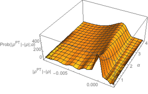
Figure 1: Density-approximation estimation based on the first 51 moments of the probability distributions, as a function of the Dyson-index-like parameter $\alpha$, of the variable ($|\rho^{PT}|-|\rho|$)

II.2.1 Probabilities over larger interval $[-\frac{1}{432},\frac{1}{432}]$

For the two-rebit, two-qubit and two-quaterbit probabilities over the extended interval $[-\frac{1}{432},\frac{1}{432}]$, symmetric about zero, containing all separable and now some entangled states (and thus providing upper bounds on the total separability probabilities), the estimates, again based on 9,451 moments were 0.78082617689, 0.69244685258 and 0.601390039979. However, we were not able to discern any particular underlying common structure (formula) in these values.

III Generic, minimally degenerate cases ($|\rho|=0$)

Let us now importantly note that these “half-separability-probabilities” of $\frac{29}{128},\frac{4}{33},\frac{13}{323}$ obtained above, appear, by Hilbert-Schmidt-based analyses of Szarek, Bengtsson and Życzkowski Szarek et al. (2006), to be exactly equal to the “full-separability-probabilities” for the corresponding minimally-degenerate (boundary, that is $|\rho|=0$) generic two-rebit, two-qubit and two-quaterbit states. We are now able to make a further interesting connection to this body of work–and thereby find additional strong support for its findings, as well as our earlier ones Slater and Dunkl (2012); Slater (2013), obtained quite independently.

Let us note, firstly, that in (Slater and Dunkl, 2012, sec. 7) it was asserted that the range of $|\rho^{PT}|$ under the minimally-degenerate constraint $|\rho|=0$ is (once again, as it was for ($|\rho^{PT}|-|\rho|)$ above) the interval $[-\frac{1}{16},\frac{1}{432}]$. (Under this determinantal constraint, we will employ the notation $|\rho_{0}^{PT}|$.) The maximum of this range is attainable by the two-parameter density matrix (4), for example, with $u=\frac{1}{6}$ and $v=\frac{1}{6}$.

In (Slater and Dunkl, 2012, App. C), we had listed the two-rebit ($\alpha=\frac{1}{2}$) Hilbert-Schmidt moments of $|\rho_{0}^{PT}|^{n}$, $n=1,\ldots,10$. Now, in an exploratory exercise, we computed the ratio of these ten results to the corresponding moments given by the $4F3$-based formula above for the moments of $(|\rho^{PT}|-|\rho|)$. Most interestingly, these ten ratios had the explanatory formula (found by the Mathematica FindSequenceFunction command)

$$\frac{(3n+7)(4n+9)}{9(4n+7)}.$$ (5)

Then, performing further computations for $\alpha=1,n=1,2$, it was possible to develop a line of reasoning (Appendix B) that the expression (5) was the $\alpha=\frac{1}{2}$-specific case of a more general moment formula, incorporating the factor

$$\frac{(10\alpha+3n+2)(12\alpha+4n+3)}{(12\alpha+3)(10\alpha+4n+2)}$$ (6)

(equaling 1 for $n=0$). In fact, the existence of a ratio of this form between the moments implies the equality of the probabilities that the respective random variables–in the case at hand, ($|\rho^{PT}|-|\rho|$) and $|\rho_{0}^{PT}|$–are positive (Appendix C).

III.1 Separability probability calculations, using density-approximation

We employed 9,451 of the original $4F3$-based moments now adjusted by this last ratio (6), in the density-approximation routine of Provost, just as before. For $\alpha=\frac{1}{2},1,\frac{3}{2}$ and 2, we obtained for the cumulative probabilities over the separability interval $[0,\frac{1}{432}]$, the values $0.50000261669\times P(\frac{1}{2})$, $0.50000003530\times P(1)$, $0.50000000060467\times P(\frac{3}{2})$ and $0.50000000001267\times P(2)$, and similarly for $\alpha>2$.

We note that the convergence of these results to $P(\alpha)/2$ is somewhat superior than in the earlier parallel set of analyses for ($|\rho^{PT}|-|\rho|$) (sec. II.2). Apparently relatedly, the ratio of the standard deviation of the probability distribution of ($|\rho^{PT}|-|\rho|$) to that of $|\rho_{0}^{PT}|$ is 0.788 for $\alpha=\frac{1}{2}$ and 0.857 for $\alpha=1$. So, the distribution for ($|\rho^{PT}|-|\rho|$) is more peaked at the value zero. Thus, the Legendre-polynomial-based density-approximation procedure (which starts with a uniform approximation) is slower to converge in those cases. Further consistent with this observation, based now on 6,301 moments, the ratio of the “$y$”-intercept for ($|\rho^{PT}|-|\rho|$) to that for $|\rho_{0}^{PT}|$ was estimated as 1.30202 for $\alpha=\frac{1}{2}$ and 1.21134 for $\alpha=1$.

III.1.1 Relations to separability-probability theorem of Szarek, Bengtsson and Życzkowski

These density approximation estimations extraordinarily close to one-half certainly are strongly in line with the main finding regarding the Hilbert-Schmidt separability probabilities of minimally degenerate (boundary) states of Szarek, Bengtsson and Życzkowski (Szarek et al., 2006, Theorem 2). These three authors had established that the set of positive-partial-transpose states for an arbitrary bipartite systems is “pyramid-decomposable” and hence, a body of “constant height”. They stated that “since our reasoning hinges directly on the Euclidean geometry, it does not allow one to predict any values of analogous ratios computed with respect to the Bures measure, nor other measures” (Szarek et al., 2006, p. L125).

Nonetheless, the “symmetric halves” separability-probability finding elucidated above (that is, the separability probability for $|\rho^{PT}|>|\rho|$ equaling that for $|\rho|>|\rho^{PT}|$) does appear to be measure-independent, that is extendible from the Hilbert-Schmidt (flat, Euclidean) metric to the use of alternative metrics, such as the Bures (minimal monotone) metric Sommers and Życzkowski (2003); Bengtsson and Życzkowski (2006).

III.1.2 Rank-two $4\times 4$ density matrices

We have also been able to conclude that for the generic rank-two $4\times 4$ density matrices (for which, of course, $|\rho|$ is also zero)–as opposed to the generic rank-three (minimally degenerate) ones just analyzed, the Hilbert-Schmidt separability probability is zero. An intuitive argument to this effect is that if one possesses a rank-two $4\times 4$ density matrix with a positive partial transpose, then if one interchanges the role of these two matrices, one has a partial transpose with two zero eigenvalues (cf. Ishizaka (2004)). Such a scenario is infinitesimally close to one with two (slightly) negative eigenvalues–a situation which has been well-established is not tenable Augusiak et al. (2008); Demianowicz (2011). (Somewhat contrastingly, in Slater (2005), numerical evidence indicated that the ratio of Hilbert-Schmidt separability probabilities for generic [rank-six] $6\times 6$ density matrices to rank-four such matrices was close to the integer 34.) A fortiori, the Hilbert-Schmidt separability probability of the generic rank-one (pure states) $4\times 4$ density matrices is also zero.

IV Concluding Remarks

In need of further study is the issue of whether or not the Dyson-index ansatz of random matrix theory Dumitriu et al. (2007); Caselle and Magnea (2004)–apparently applicable in the Hilbert-Schmidt case, as our various results for general $\alpha$ so far would indicate–extends to other measures (Bures,…), as well (cf. Slater (2012, )).

We note, regretfully, of course, that formal proofs for the Hilbert-Schmidt determinantal moment formulas and the density-approximation results obtained with their use have not yet been advanced–and certainly still seem far from development. Certainly, however, the cumulative computational evidence appears very strong for the validity of, inter alia, the indicated $\frac{29}{64},\frac{8}{33}$ and $\frac{26}{323}$ two-rebit, two-qubit and two-quaterbit separability probabilities. Noticeably still lacking is an insightful geometric intuition into the geometry of the $4\times 4$ density matrices that might help to explain such results (cf. Avron et al. (2007); Avron and Kenneth (2009); Holik and Plastino (2011); Milne et al. ; Sarbicki and Bengtsson (2013)). Can the $\frac{8}{33}$ two-qubit separability probability result, for example, only be understood in some sense as a limiting result–as the infinite-summation “concise formula” ((1)-(3)) might seem to indicate–or is it possibly remarkably manifest in some discrete (pyramidal? Szarek et al. (2006)) subdivision of the 15-dimensional convex set of $4\times 4$ density matrices?

Possible extensions of the research program presented above and in Slater and Dunkl (2012); Slater (2013) to the Hilbert-Schmidt case of $6\times 6$ (qubit-qutrit) density matrices and the Bures instance of $4\times 4$ density matrices have been investigated in Slater (2012, ). Some limited determinantal moment computations have been reported ($\alpha=\frac{1}{2}$, $n=1,2$; $\alpha=1$, $n=1$, in both instances) (Appendix D), but yet no comparable formulas of the type $\left\langle\left|\rho\right|^{k}\left|\rho^{PT}\right|^{n}\right\rangle/\left\langle\left|\rho\right|^{k}\right\rangle$ nor $\left\langle\left|\rho\right|^{k}(\left|\rho^{PT}\right|-|\rho|)^{n}\right\rangle/\left\langle\left|\rho\right|^{k}\right\rangle$ developed. Such formulas have been the fundamental basis for most of the advances noted here and previously Slater and Dunkl (2012); Slater (2013).

Appendix A: Moments of $\left(\left|\rho^{PT}\right|-\left|\rho\right|\right)$

Consider the general $\alpha$ case, generic $k$.

Let

$$g\left(k,n\right):=\frac{\left(k+1\right)_{n}\left(k+1+\alpha\right)_{n}\left(k+1+2\alpha\right)_{n}}{2^{6n}\left(k+3\alpha+\frac{3}{2}\right)_{n}\left(2k+6\alpha+\frac{5}{2}\right)_{2n}},$$

there is a multiplication relation:

$$g\left(0,k\right)g\left(k,n\right)=g\left(0,k+n\right).$$

Let

$$h\left(k,n\right):=~{}_{5}F_{4}\left(\genfrac{}{}{0.0pt}{}{-n,-k,\alpha,\alpha+\frac{1}{2},-2k-2n-1-5\alpha}{-k-n-\alpha,-k-n-2\alpha,-\frac{k+n}{2},-\frac{k+n-1}{2}};1\right).$$

Then

$$\left\langle\left|\rho\right|^{k}\right\rangle =g\left(0,k\right)$$

$$\left\langle\left|\rho^{PT}\right|^{n}\left|\rho\right|^{k}\right\rangle/\left\langle\left|\rho\right|^{k}\right\rangle =g\left(k,n\right)h\left(k,n\right)$$

$$\left\langle\left|\rho^{PT}\right|^{n}\left|\rho\right|^{k}\right\rangle =g\left(0,k+n\right)h\left(k,n\right).$$

Define

$$F_{2}\left(n,k\right)=\left\langle\left|\rho\right|^{k}\left(\left|\rho^{PT}\right|-\left|\rho\right|\right)^{n}\right\rangle/\left\langle\left|\rho\right|^{k}\right\rangle,$$

then

$$F_{2}\left(n,k\right) =\frac{1}{g\left(0,k\right)}\sum_{j=0}^{n}\binom{n}{j}\left(-1\right)^{n-j}\left\langle\left|\rho\right|^{k+n-j}\left|\rho^{PT}\right|^{j}\right\rangle$$

$$=\frac{1}{g\left(0,k\right)}\sum_{j=0}^{n}\binom{n}{j}\left(-1\right)^{n-j}g\left(0,k+n\right)h\left(k+n-j,j\right)$$

$$=g\left(k,n\right)\sum_{j=0}^{n}\binom{n}{j}\left(-1\right)^{n-j}h\left(k+n-j,j\right).$$

We will produce $F_{2}^{\prime}\left(n,k\right):=\sum_{j=0}^{n}\binom{n}{j}\left(-1\right)^{n-j}h\left(k+n-j,j\right)$ as a single sum (so that $F_{2}\left(n,k\right)=g\left(k,n\right)F_{2}^{\prime}\left(n,k\right)$).

Lemma IV.1

Let $n,m=0,1,2,\ldots$ and let $x$ be a variable, if $0\leq m\leq n$ then

$$\sum_{j=0}^{n}\frac{\left(-n\right)_{j}}{j!}\left(-j\right)_{m}\left(x+j\right)_{m}=\left(-1\right)^{m}\frac{\left(x\right)_{2m}}{\left(x\right)_{n}}\left(-n\right)_{m}\left(-m\right)_{n-m},$$

otherwise the sum is zero.

• If $m>n$ then $\left(-j\right)_{m}=0$ for $0\leq j\leq n$. Suppose $0\leq m\leq n$ then $\left(-j\right)_{m}=0$ for $0\leq j<m$ and the sum is over $m\leq j\leq n$. Thus

  $$\sum_{j=m}^{n}\frac{\left(-n\right)_{j}}{j!}\left(-j\right)_{m}\left(x+j\right)_{m} =\left(-1\right)^{m}\sum_{j=m}^{n}\frac{\left(-n\right)_{j}~{}j!}{j!\left(j-m\right)!}\frac{\left(x\right)_{j}\left(x+j\right)_{m}}{\left(x\right)_{j}}$$

  $$=\left(-1\right)^{m}\left(x\right)_{m}\sum_{j=m}^{n}\frac{\left(-n\right)_{j}\left(x+m\right)_{j}}{\left(j-m\right)!\left(x\right)_{j}}.$$

  Change the index of summation $j=m+i$ then the sum equals

  $$\left(-1\right)^{m}\frac{\left(-n\right)_{m}\left(x\right)_{m}\left(x+m\right)_{m}}{\left(x\right)_{m}}\sum_{i=0}^{n-m}\frac{\left(m-n\right)_{i}\left(x+2m\right)_{i}}{i!\left(x+m\right)_{i}}$$

  $$=\left(-1\right)^{m}\frac{\left(-n\right)_{m}\left(x\right)_{2m}}{\left(x\right)_{m}}\frac{\left(-m\right)_{n-m}}{\left(x+m\right)_{n-m}}$$

  $$=\left(-1\right)^{m}\left(-n\right)_{m}\left(-m\right)_{n-m}\frac{\left(x\right)_{2m}}{\left(x\right)_{n}},$$

  by the Chu-Vandermonde sum.

Observe that $\left(-m\right)_{n-m}=0$ for $2m<n$. Then

$$F_{2}^{\prime}\left(n,k\right) =\left(-1\right)^{n}\sum_{j=0}^{n}\frac{\left(-n\right)_{j}}{j!}$$

$$\times\sum_{i=0}^{n}\frac{\left(-j\right)_{i}\left(j-k-n\right)_{i}\left(\alpha\right)_{i}\left(\alpha+\frac{1}{2}\right)_{i}\left(-2k-2n-1-5\alpha\right)_{i}}{i!\left(-k-n-\alpha\right)_{i}\left(-k-n-2\alpha\right)_{i}\left(-\frac{k+n}{2}\right)_{i}\left(-\frac{k+n-1}{2}\right)_{i}}$$

$$=\left(-1\right)^{n}\sum_{i=0}^{n}\frac{\left(\alpha\right)_{i}\left(\alpha+\frac{1}{2}\right)_{i}\left(-2k-2n-1-5\alpha\right)_{i}}{i!\left(-k-n-\alpha\right)_{i}\left(-k-n-2\alpha\right)_{i}\left(-\frac{k+n}{2}\right)_{i}\left(-\frac{k+n-1}{2}\right)_{i}}$$

$$\times\sum_{j=0}^{n}\frac{\left(-n\right)_{j}}{j!}\left(-j\right)_{i}\left(j-k-n\right)_{i}.$$

Apply the lemma to the $j$-sum with $x=-k-n$ and $m=i$ to obtain

$$\left(-1\right)^{i}\left(-n\right)_{i}\left(-i\right)_{n-i}\frac{\left(-n-k\right)_{2i}}{\left(-n-k\right)_{n}}=\left(-1\right)^{i}\frac{\left(-n\right)_{i}\left(-i\right)_{n-i}}{\left(-n-k\right)_{n}}2^{2i}\left(-\frac{k+n}{2}\right)_{i}\left(-\frac{k+n-1}{2}\right)_{i}$$

and thus

$$F_{2}^{\prime}\left(n,k\right)=\frac{\left(-1\right)^{n}}{\left(-n-k\right)_{n}}\sum_{i=0}^{n}\frac{\left(-n\right)_{i}\left(-i\right)_{n-i}\left(\alpha\right)_{i}\left(\alpha+\frac{1}{2}\right)_{i}\left(-2k-2n-1-5\alpha\right)_{i}}{i!\left(-k-n-\alpha\right)_{i}\left(-k-n-2\alpha\right)_{i}}\left(-1\right)^{i}2^{2i}.$$

This is not in hypergeometric form because of the term $\left(-i\right)_{n-i}$; also the summation extends over $\frac{n}{2}\leq i\leq n$. Change the index $j=n-i$ then

$$\frac{\left(-n\right)_{i}}{i!}\left(-i\right)_{n-i} =\left(-1\right)^{i}\frac{n!}{\left(n-i\right)!i!}\left(-1\right)^{n-i}\frac{i!}{\left(2i-n\right)!}=\left(-1\right)^{n}\frac{n!}{j!\left(n-2j\right)!}$$

$$=\left(-1\right)^{n}\frac{2^{2j}}{j!}\left(-\frac{n}{2}\right)_{j}\left(\frac{1-n}{2}\right)_{j}$$

and the reversal formula is

$$\left(x\right)_{i} =\left(x\right)_{n-j}=\frac{\left(x\right)_{n-j}\left(x+n-j\right)_{j}}{\left(x+n-j\right)_{j}}$$

$$=\left(-1\right)^{j}\frac{\left(x\right)_{n}}{\left(1-n-x\right)_{j}}.$$

Thus

$$F_{2}^{\prime}\left(n,k\right) =\frac{\left(-1\right)^{n}\left(\alpha\right)_{n}\left(\alpha+\frac{1}{2}\right)_{n}\left(-2k-2n-1-5\alpha\right)_{n}}{\left(-n-k\right)_{n}\left(-k-n-\alpha\right)_{n}\left(-k-n-2\alpha\right)_{n}}$$ (7)

$$\times\sum_{j=0}^{[n/2]}\frac{\left(-\frac{n}{2}\right)_{j}\left(\frac{1-n}{2}\right)_{j}\left(k+1+\alpha\right)_{j}\left(k+1+2\alpha\right)_{j}}{j!\left(1-n-\alpha\right)_{j}\left(\frac{1}{2}-n-\alpha\right)_{j}\left(n+2k+2+5\alpha\right)_{j}}2^{2j+2n-2j}$$

$$=\left(-1\right)^{n}2^{2n}\frac{\left(\alpha\right)_{n}\left(\alpha+\frac{1}{2}\right)_{n}\left(n+2k+2+5\alpha\right)_{n}}{\left(k+1\right)_{n}\left(k+1+\alpha\right)_{n}\left(k+1+2\alpha\right)_{n}}$$

$$\times~{}_{4}F_{3}\left(\genfrac{}{}{0.0pt}{}{-\frac{n}{2},\frac{1-n}{2},k+1+\alpha,k+1+2\alpha}{1-n-\alpha,\frac{1}{2}-n-\alpha,n+2k+2+5\alpha};1\right);$$

a balanced sum.

The formula was tested for $F_{2}\left(2,k\right)$, also directly verified for $n=3$, arbitrary $\alpha$.

Combining the front factors in $F_{2}\left(n,k\right)$ (from $g\left(k,n\right)$) we obtain

$$\left(-1\right)^{n}\frac{\left(\alpha\right)_{n}\left(\alpha+\frac{1}{2}\right)_{n}\left(n+2k+2+5\alpha\right)_{n}}{2^{4n}\left(k+3\alpha+\frac{3}{2}\right)_{n}\left(2k+6\alpha+\frac{5}{2}\right)_{2n}}.$$ (8)

Appendix B: Minimally degenerate case

Recall the Cholesky decomposition $\rho=C^{\ast}C$ where

$$C=\begin{bmatrix}x_{1}&x_{5}&x_{6}&x_{7}\\ 0&x_{2}&x_{8}&x_{9}\\ 0&0&x_{3}&x_{10}\\ 0&0&0&x_{4}\end{bmatrix}$$ (9)

with $\sum_{j=1}^{10}\left|x_{j}\right|^{2}=1,x_{j}\geq 0$ for $1\leq j\leq 4$ and $x_{j}\in\mathbb{R}$ for $\alpha=\frac{1}{2}$, or $x_{j}\in\mathbb{C}$ for $\alpha=1$ ($5\leq j\leq 10$). Then $\left|\rho\right|=\left(x_{1}x_{2}x_{3}x_{4}\right)^{2}$. Denote integration over the space of $4\times 4$ positive-definite matrices with trace one by $\left\langle\cdot\right\rangle$. Suppose $p$ is a monomial in $\left\{x_{j},\overline{x_{j}}\right\}$ then

$$\left\langle p\right\rangle=\frac{\left(1+3\alpha\right)_{n_{1}}\left(1+2\alpha\right)_{n_{2}}\left(1+\alpha\right)_{n_{3}}\left(1\right)_{n_{4}}}{\left(4+12\alpha\right)_{n}}\prod_{j=5}^{10}\left(\alpha\right)_{n_{j}}$$ (10)

where $n=\sum_{j=1}^{10}n_{j}$ and:

• $\alpha=\frac{1}{2},~{}p=\prod_{j=1}^{10}x_{j}^{2n_{j}}$, that is, each exponent is even;

• $\alpha=1,~{}p=\prod_{j=1}^{4}x_{j}^{2n_{j}}\times\prod_{j=5}^{10}\left(x_{j}\overline{x_{j}}\right)^{n_{j}}$, that is, $p$ is a monomial in $x_{1}^{2},\cdots,x_{4}^{2},\left|x_{5}\right|^{2},\cdots,\left|x_{10}\right|^{2}$;

otherwise $\left\langle p\right\rangle=0$.

The boundary of the set of states (positive-definite matrices with trace one) contains $\Omega_{0}$, the set of positive-semidefinite matrices of possible ranks $1,2$ or $3$ (and trace one). In the following discussion the parameters are stated first for the real $\alpha=\frac{1}{2}$ case, then in parentheses for the complex $\alpha=1$ case. We consider the determinant of the partial transpose, denoted by $\left|\rho_{0}^{PT}\right|$, as a random variable defined on $\Omega_{0}$, with respect to the Hilbert-Schmidt measure, that is, the Euclidean $8$-dimensional (resp. $14$) measure, restricted to $\Omega_{0}$. We claim that integrating with respect to this measure can be carried out by integrating over Cholesky products with $x_{4}=0$ and the surface measure on the unit sphere in $\mathbb{R}^{9}$ (resp. $\mathbb{R}^{15}$) and the Jacobian $x_{1}^{5/2}x_{2}^{2}x_{3}^{3/2}$ (resp. $x_{1}^{4}x_{2}^{3}x_{3}^{2}$). The generic (or random) elements of $\Omega_{0}$ are called minimally degenerate.

Let $\Omega_{0}^{C}$ denote the set of Cholesky products $C^{\ast}C$ with the conditions as in (9) and with $x_{4}=0$. The same arguments used in (Slater and Dunkl, 2012, sec. D.2) show that the surface measure on the sphere multiplied by the above Jacobian is mapped to the HS-measure on $\Omega_{0}^{C}$. So it remains to show that the elements of $\Omega_{0}\backslash\Omega_{0}^{C}$ do not enter into the probability calculation. For any real symmetric (resp. Hermitian) $4\times 4$ matrix $M$ let $d_{j}\left(M\right)$ denote the determinant of the upper left $j\times j$ submatrix of $M$ (a principal minor), for $1\leq j\leq 4$. Then $M$ is positive-definite (resp. positive-semidefinite) if and only if $d_{j}\left(M\right)>0$ for all $j$ (resp. $d_{j}\left(M\right)\geq 0$ for all $j$). Suppose $\rho\in\Omega_{0}$ then $\rho$ has a unique Cholesky factorization if $d_{j}\left(\rho\right)>0$ for $j=1,2,3$; these conditions imply that $x_{1}x_{2}x_{3}>0$. As a consequence $x_{4}=0$ because $\left|\rho\right|=\left(x_{1}x_{2}x_{3}x_{4}\right)^{2}$, and thus $\rho\in\Omega_{0}^{C}$.

As contrapositive we have shown that $\rho\in\Omega_{0}\backslash\Omega_{0}^{C}$ implies $d_{j}\left(\rho\right)=0$ for at least one value of $j=1,2,3$. This is an additional algebraic condition besides $\left|\rho\right|=0$ satisfied by the entries of $\rho$, that is $\rho$ belongs to a manifold (or variety) of lower dimension in $\Omega_{0}$ ($<8$ for $\alpha=\frac{1}{2}$, and $<14$ for $\alpha=1$) and such sets have HS-measure zero.

The appropriate measure on the set of Cholesky factors with $x_{4}=0$ can be interpreted as a conditional density on a subset of the unit sphere, or as the surface measure on the sphere in one less dimension. In general suppose $f$ is a density on some region $E\subset\mathbb{R}^{N}$ then the conditional density given $y_{N}=u$ is

$$\frac{f\left(y_{1},\cdots,y_{N-1},u\right)}{\int_{E_{u}}f\left(t_{1},\cdots,t_{N-1},u\right)dt_{1}\cdots dt_{N-1}}$$

where $E_{u}:=\left\{t\in\mathbb{R}^{N-1}:\left(t,u\right)\in E\right\}$. In our situation the density vanishes on the set of interest ($x_{4}=0$) so we need to take a limit.

Consider a general Dirichlet density

$$\frac{\Gamma\left(\alpha_{1}+\cdots+\alpha_{N}\right)}{\Gamma\left(\alpha_{1}\right)\cdots\Gamma\left(\alpha_{N}\right)}\prod_{j=1}^{N}y_{j}^{\alpha_{j}-1}$$

on $T_{N-1}=\left\{y\in\mathbb{R}_{N-1}:y_{j}\geq 0~{}\forall j,\sum_{j=1}^{N-1}y_{j}\leq 1\right\}$ and $y_{N}:=1-\sum_{j=1}^{N-1}y_{j}$; also $\alpha_{j}>0~{}\forall j$. Compute the conditional density given $x_{N}=u$ with $0<u<1$; then $E_{u}=\left(1-u\right)T_{N-2}$, that is, $E_{u}=\left\{y\in\mathbb{R}_{N-2}:y_{j}\geq 0~{}\forall j,\sum_{j=1}^{N-2}y_{j}\leq 1-u\right\}$. After a simple change-of-variable we obtain the conditional density

$$\frac{\Gamma\left(\alpha_{1}+\cdots+\alpha_{N-1}\right)}{\Gamma\left(\alpha_{1}\right)\cdots\Gamma\left(\alpha_{N-1}\right)\left(1-u\right)^{\beta-1}}\prod_{j=1}^{N-2}y_{j}^{\alpha_{j}-1},$$

where $\beta=\sum_{j=1}^{N-1}\alpha_{j},y\in E_{u}$ and $y_{N-1}:=1-u-\sum_{j=1}^{N-2}y_{j}$. Now we can take the limit $u\rightarrow 0_{+}$ and obtain the obvious Dirichlet distribution on $T_{N-2}$.

By applying this general result to the Cholesky factor (where $y_{j}=x_{j}^{2}$ or $\left|x_{j}\right|^{2}$ and $N=10,16$ for $\alpha=\frac{1}{2},1$ respectively) we find that the formula for the integral of a monomial with respect to the ($x_{4}=0$)-conditional density is very similar to the general one

$$\left\langle p\right\rangle=\frac{\left(1+3\alpha\right)_{n_{1}}\left(1+2\alpha\right)_{n_{2}}\left(1+\alpha\right)_{n_{3}}\left(0\right)_{n_{4}}}{\left(3+12\alpha\right)_{n}}\prod_{j=5}^{10}\left(\alpha\right)_{n_{j}},$$ (11)

with the same rules for $n_{i}$ as before; the effect of the term $\left(0\right)_{n_{4}}$ is that $\left\langle p\right\rangle=0$ for any monomial having $x_{4}$ as a factor; note $\left(0\right)_{0}=1$ (the empty product).

We proceed to the main results (conjectures): there is a natural decomposition

$$\left|\rho^{PT}\right|=f_{1}\left(x^{\prime}\right)+x_{4}^{2}f_{2}\left(x^{\prime}\right)+\left|\rho\right|,$$

where $x^{\prime}$ omits $x_{4}$ (that is, $x^{\prime}=\left(x_{1},\cdots,x_{3},x_{5},\cdots,x_{10}\right)$). In the previous section there is a formula for $\left\langle\left|\rho\right|^{k}\left(\left|\rho^{PT}\right|-\left|\rho\right|\right)^{n}\right\rangle=\left\langle\left|\rho\right|^{k}\left(f_{1}\left(x^{\prime}\right)+x_{4}^{2}f_{2}\left(x^{\prime}\right)\right)^{n}\right\rangle$. Note $f_{1}\left(x^{\prime}\right)=\left|\rho_{0}^{PT}\right|$ when $\rho\in\Omega_{0}^{C}$. It is desired to find $\left\langle f_{1}\left(x^{\prime}\right)^{n}\right\rangle$, namely the $n^{th}$ moment of $\left|\rho_{0}^{PT}\right|$, for the conditional density (11). The key step is to consider

$$\left\langle\left(x_{1}x_{2}x_{3}\right)^{2k}x_{4}^{2k-2}\left(f_{1}\left(x^{\prime}\right)+x_{4}^{2}f_{2}\left(x^{\prime}\right)\right)^{n}\right\rangle,$$

for $k=1,2,3,\ldots$ ($k>0$ is required for integrability). Consider the integrals of monomials (notations as in (10)):

$$\left\langle\left(x_{1}x_{2}x_{3}x_{4}\right)^{2k}p\right\rangle=\frac{\left(1+3\alpha\right)_{k}\left(1+2\alpha\right)_{k}\left(1+\alpha\right)_{k}\left(1\right)_{k}}{\left(4+12\alpha\right)_{4k}}$$ (12)

$$\times\frac{\left(k+1+3\alpha\right)_{n_{1}}\left(k+1+2\alpha\right)_{n_{2}}\left(k+1+\alpha\right)_{n_{3}}\left(k+1\right)_{n_{4}}}{\left(4+4k+12\alpha\right)_{n}}\prod_{j=5}^{10}\left(\alpha\right)_{n_{j}},$$ (13)

and

$$\left\langle\left(x_{1}x_{2}x_{3}\right)^{2k}x_{4}^{2k-2}p\right\rangle=\frac{\left(1+3\alpha\right)_{k}\left(1+2\alpha\right)_{k}\left(1+\alpha\right)_{k}\left(1\right)_{k-1}}{\left(4+12\alpha\right)_{4k-1}}$$ (14)

$$\times\frac{\left(k+1+3\alpha\right)_{n_{1}}\left(k+1+2\alpha\right)_{n_{2}}\left(k+1+\alpha\right)_{n_{3}}\left(k\right)_{n_{4}}}{\left(3+4k+12\alpha\right)_{n}}\prod_{j=5}^{10}\left(\alpha\right)_{n_{j}}.$$ (15)

Observe that the quantity on the right side of (12) is $\left\langle\left|\rho\right|^{k}\right\rangle$ and the quantity on the right side of (14) is $\left\langle\left(x_{1}x_{2}x_{3}\right)^{2k}x_{4}^{2k-2}\right\rangle$.
Conjecture
For $k=1,2,3,\ldots,\alpha=\frac{1}{2}$ or $1$

$$\left\langle\left(x_{1}x_{2}x_{3}\right)^{2k}x_{4}^{2k-2}\left(\left|\rho^{PT}\right|-\left|\rho\right|\right)^{n}\right\rangle=\left\langle\left(x_{1}x_{2}x_{3}\right)^{2k}x_{4}^{2k-2}\right\rangle$$

$$\times\frac{\left(2+4k+10\alpha+3n\right)\left(3+4k+12\alpha+4n\right)}{\left(2+4k+10\alpha+4n\right)\left(3+4k+12\alpha\right)}F_{2}\left(n,k\right),$$

where $F_{2}$ is given in (7) and (8).

The conjectured formula can be written as

$$\frac{\left\langle\left(x_{1}x_{2}x_{3}\right)^{2k}x_{4}^{2k-2}\left(f_{1}\left(x^{\prime}\right)+x_{4}^{2}f_{2}\left(x^{\prime}\right)\right)^{n}\right\rangle}{\left\langle\left(x_{1}x_{2}x_{3}\right)^{2k}x_{4}^{2k-2}\right\rangle}$$

$$=\left(-1\right)^{n}\frac{\left(\alpha\right)_{n}\left(\alpha+\frac{1}{2}\right)_{n}\left(n+2k+1+5\alpha\right)_{n}\left(2+10\alpha+4k+3n\right)}{2^{4n}\left(k+3\alpha+\frac{3}{2}\right)_{n}\left(2k+6\alpha+\frac{3}{2}\right)_{2n}\left(2+10\alpha+4k+2n\right)}$$

$$\times~{}_{4}F_{3}\left(\genfrac{}{}{0.0pt}{}{-\frac{n}{2},\frac{1-n}{2},k+1+\alpha,k+1+2\alpha}{1-n-\alpha,\frac{1}{2}-n-\alpha,n+2k+2+5\alpha};1\right).$$

Corollary IV.2

The ($x_{4}=0$)-conditional expectation

$$\left\langle f_{1}\left(x^{\prime}\right)^{n}\right\rangle =\left\langle\left|\rho_{0}^{PT}\right|^{n}\right\rangle$$

$$=\left(-1\right)^{n}\frac{\left(\alpha\right)_{n}\left(\alpha+\frac{1}{2}\right)_{n}\left(n+1+5\alpha\right)_{n}\left(2+10\alpha+3n\right)}{2^{4n}\left(3\alpha+\frac{3}{2}\right)_{n}\left(6\alpha+\frac{3}{2}\right)_{2n}\left(2+10\alpha+2n\right)}$$

$$\times~{}_{4}F_{3}\left(\genfrac{}{}{0.0pt}{}{-\frac{n}{2},\frac{1-n}{2},1+\alpha,1+2\alpha}{1-n-\alpha,\frac{1}{2}-n-\alpha,n+2+5\alpha};1\right).$$

• From (14) and (15), for a monomial $p$ we have

  $$\frac{\left\langle\left(x_{1}x_{2}x_{3}\right)^{2k}x_{4}^{2k-2}p\right\rangle}{\left\langle\left(x_{1}x_{2}x_{3}\right)^{2k}x_{4}^{2k-2}\right\rangle}=\frac{\left(k+1+3\alpha\right)_{n_{1}}\left(k+1+2\alpha\right)_{n_{2}}\left(k+1+\alpha\right)_{n_{3}}\left(k\right)_{n_{4}}}{\left(3+4k+12\alpha\right)_{n}}\prod_{j=5}^{10}\left(\alpha\right)_{n_{j}},$$

  with the same conditions on $\left\{n_{i}\right\}$ as before. The limit of this expression as $k\rightarrow 0_{+}$ equals the ($x_{4}=0$)-conditional expectation $\left\langle p\right\rangle$. From the property of $\left(0\right)_{n_{4}}$ it follows that $\left\langle\left(f_{1}\left(x^{\prime}\right)+x_{4}^{2}f_{2}\left(x^{\prime}\right)\right)^{n}\right\rangle=\left\langle f_{1}\left(x^{\prime}\right)^{n}\right\rangle$.

The conjecture has been verified (by symbolic computation) for $n=1,2,3,4$, $\alpha=\frac{1}{2}$ and $\alpha=1$. (One notes that the $n=4,\alpha=1$ computation involves around 8000 monomials with a nonzero integral, and roughly 4 million monomials with zero integral. Each of these monomials is of degree 32 in 16 variables.)

Appendix C: Equal probabilities

For a probability density supported on a bounded interval $I$ let $\mu_{n}\left[f\right]:=\int_{I}x^{n}f\left(x\right)dx,$ for $n=0,1,2,\ldots$. The following is the probability density for the random variable $XY$ where the density function of $X$ is $f\left(x\right)$, the density of $Y$ is $\gamma y^{\gamma-1}$ on $0<y<1,$ and $X,Y$ are independent. It is obvious that $\Pr\left\{XY>0\right\}=\Pr\left\{X>0\right\}$.

• Suppose $f\left(x\right)$ is a probability density function supported on $\left[a,b\right]$ with $a<0<b$, and $\gamma>0$, then

  $$M\left(\gamma\right)f\left(x\right):=\left\{\begin{array}[c]{c}\gamma x^{\gamma-1}\int_{x}^{b}f\left(t\right)t^{-\gamma}dt,~{}0<x<b\\ \gamma\left|x\right|^{\gamma-1}\int_{a}^{x}f\left(t\right)\left|t\right|^{-\gamma}dt,~{}a<x<0.\end{array}\right.$$

Proposition IV.3

Suppose $f,\gamma$ are as in the definition, and $n=0,1,2,3,\ldots$ then $M\left(\gamma\right)f$ is a probability density such that

$$\int_{0}^{b}x^{n}M\left(\gamma\right)f\left(x\right)dx =\frac{\gamma}{\gamma+n}\int_{0}^{b}x^{n}f\left(x\right)dx,$$

$$\int_{a}^{0}x^{n}M\left(\gamma\right)f\left(x\right)dx =\frac{\gamma}{\gamma+n}\int_{a}^{0}x^{n}f\left(x\right)dx,$$

$$\mu_{n}\left[M\left(\gamma\right)f\right] =\frac{\gamma}{\gamma+n}\mu_{n}\left[f\right].$$

• In the following iterated integral change the order of integration and then evaluate the inner integral:

  $$\int_{0}^{b}x^{n}M\left(\gamma\right)f\left(x\right)dx =\gamma\int_{0}^{b}x^{n+\gamma-1}dx\int_{x}^{b}f\left(t\right)t^{-\gamma}dt=\gamma\int_{0}^{b}f\left(t\right)t^{-\gamma}dt\int_{0}^{t}x^{n+\gamma-1}dx$$

  $$=\frac{\gamma}{\gamma+n}\int_{0}^{b}f\left(t\right)t^{-\gamma+n+\gamma}dt.$$

  Similarly

  $$\int_{a}^{0}x^{n}M\left(\gamma\right)f\left(x\right)dx =\gamma\int_{a}^{0}x^{n}\left|x\right|^{\gamma-1}dx\int_{a}^{x}f\left(t\right)\left|t\right|^{-\gamma}dt$$

  $$=\gamma\int_{a}^{0}f\left(t\right)\left|t\right|^{-\gamma}dt\int_{t}^{0}x^{n}\left|x\right|^{\gamma-1}dx;$$

  in the inner integral change the variable $x=-u$ and then integrate to obtain $\left(-1\right)^{n}\dfrac{\left(-t\right)^{n+\gamma}}{\gamma+n}=\dfrac{t^{n}\left|t\right|^{\gamma}}{\gamma+n}$ for $a<t<0$. This establishes the first two equations and the sum of the two shows $\mu_{n}\left[M\left(\gamma\right)f\right]=\frac{\gamma}{\gamma+n}\mu_{n}\left[f\right]$.

Proposition IV.4

Suppose $f$ is a density function on $\left[a,b\right]$ with $a<0<b,$ $\gamma>0$ and $0<\delta<1$, then $g\left(x\right):=\delta f\left(x\right)+\left(1-\delta\right)M\left(\gamma\right)f\left(x\right)$ is a density function on $\left[a,b\right]$ and

$$\int_{0}^{b}x^{n}g\left(x\right)dx =\frac{\gamma+\delta n}{\gamma+n}\int_{0}^{b}x^{n}f\left(x\right)dx,$$

$$\int_{a}^{0}x^{n}g\left(x\right)dx =\frac{\gamma+\delta n}{\gamma+n}\int_{a}^{0}x^{n}f\left(x\right)dx,$$

$$\mu_{n}\left[g\right] =\frac{\gamma+\delta n}{\gamma+n}\mu_{n}\left[f\right].$$

• It is clear that $g$ is a density. The other claims follow from the previous proposition. For example

  $$\int_{0}^{b}x^{n}g\left(x\right)dx =\delta\int_{0}^{b}x^{n}f\left(x\right)dx+\left(1-\delta\right)\int_{0}^{b}x^{n}M\left(\gamma\right)f\left(x\right)dx$$

  $$=\left\{\delta+\left(1-\delta\right)\frac{\gamma}{\gamma+n}\right\}\int_{0}^{b}x^{n}f\left(x\right)dx$$

  $$=\frac{\gamma+\delta n}{\gamma+n}\int_{0}^{b}x^{n}f\left(x\right)dx.$$

Now fix $\alpha$ ($=\frac{1}{2},1$ for the real and complex cases) and denote the density function of $\left(\left|\rho^{PT}\right|-\left|\rho\right|\right)$ by $f\left(x\right)$, supported on $\left[-\frac{1}{16},\frac{1}{432}\right]$, or for arbitrary $\alpha>0$ take the density function whose $n^{th}$ moments are given by $F_{2}\left(n,0\right)$ (see equations 7 and 8 ); also denote the density function of $\left|\rho_{0}^{PT}\right|$ in the minimally degenerate setting by $g\left(x\right)$ (more generally the density whose moments are given by $\dfrac{\left(2+10\alpha+3n\right)\left(3+12\alpha+4n\right)}{\left(2+10\alpha+4n\right)\left(3+12\alpha\right)}F_{2}\left(n,0\right)$).

Let $U_{1}$ denote the random variable with density $M\left(3\alpha+\frac{3}{4}\right)g\left(x\right)$, then by Proposition IV.3 the range of $U_{1}$ is $\left[-\frac{1}{16},\frac{1}{432}\right]$ and

$$\mu_{n}\left[M\left(3\alpha+\frac{3}{4}\right)g\right] =\frac{3\alpha+\frac{3}{4}}{3\alpha+\frac{3}{4}+n}\mu_{n}\left[g\right]=\frac{3+12\alpha}{3+12\alpha+4n}\mu_{n}\left[g\right],~{}n=0,1,2,3,\ldots$$

$$\Pr\left\{U_{1}>0\right\} =\Pr\left\{\left|\rho_{0}^{PT}\right|>0\right\}.$$

Let $U_{2}$ denote the random variable with density $h\left(x\right):=\frac{3}{4}f\left(x\right)+$ $\frac{1}{4}M\left(\frac{1+5\alpha}{2}\right)f\left(x\right)$, then by Proposition IV.4 the range of $U_{2}$ is $\left[-\frac{1}{16},\frac{1}{432}\right]$ and

$$\mu_{n}\left[h\right] =\frac{\frac{1+5\alpha}{2}+\frac{3n}{4}}{\frac{1+5\alpha}{2}+n}\mu_{n}\left[f\right]=\frac{2+10\alpha+3n}{2+10\alpha+4n}\mu_{n}\left[f\right],~{}n=0,1,2,3,\ldots,$$

$$\Pr\left\{U_{2}>0\right\} =\Pr\left\{\left|\rho^{PT}\right|-\left|\rho\right|>0\right\}.$$

Proposition IV.5

Suppose $\alpha>0$ then $\Pr\left\{\left|\rho^{PT}\right|-\left|\rho\right|>0\right\}=\Pr\left\{\left|\rho_{0}^{PT}\right|>0\right\}$.

• From the conjecture it follows that $\mu_{n}\left[M\left(3\alpha+\frac{3}{4}\right)g\right]=\mu_{n}\left[h\right]$ for all $n$. By the uniqueness of moments (on bounded intervals) $U_{1}$ and $U_{2}$ have the same density and $\Pr\left\{\left|\rho^{PT}\right|-\left|\rho\right|>0\right\}=\Pr\left\{U_{2}>0\right\}=\Pr\left\{\left|\rho_{0}\right|^{PT}>0\right\}$.

Appendix D: Specific moments for $6\times 6$ Hilbert-Schmidt and $4\times 4$ Bures scenarios
$6\times 6$ Hilbert-Schmidt moments
$n=1$

$$\frac{\left\langle|\rho|^{k}(|\rho^{PT}|-|\rho|)\right\rangle_{rebit-retrit/HS}}{\left\langle|\rho|^{k}\right\rangle_{rebit-retrit/HS}}=-\frac{5(k+2)(k+3)(2k+7)}{96(k+4)(3k+11)(3k+13)(6k+23)(6k+25)},$$ (16)

$$\frac{\left\langle|\rho|^{k}(|\rho^{PT}|-|\rho|)\right\rangle_{qubit-qutrit/HS}}{\left\langle|\rho|^{k}\right\rangle_{qubit-qutrit/HS}}=-\frac{(k+3)(k+5)(2k+11)}{3(2k+13)(3k+19)(3k+20)(6k+37)(6k+41)},$$ (17)

and

$$\frac{\left\langle|\rho|^{k}(|\rho^{PT}|-|\rho|)\right\rangle_{quaterbit-quatertrit/HS}}{\left\langle|\rho|^{k}\right\rangle_{quaterbit-quatertrit/HS}}=-\frac{5(k(k(3k+70)+521)+1194)}{6(2k+23)(3k+34)(3k+35)(6k+67)(6k+71)}.$$ (18)

$n=2$

$$\frac{\left\langle|\rho|^{k}(|\rho^{PT}|-|\rho|)^{2}\right\rangle_{rebit-retrit/HS}}{\left\langle|\rho|^{k}\right\rangle_{rebit-retrit/HS}}=$$ (19)

$$\frac{5\left(24k^{6}+900k^{5}+10974k^{4}+63561k^{3}+193602k^{2}+302033k+192132\right)}{82944(k+5)(3k+11)(3k+13)(3k+14)(3k+16)(6k+23)(6k+25)(6k+29)(6k+31)}$$

and

$$\frac{\left\langle|\rho|^{k}(|\rho^{PT}|-|\rho|)^{2}\right\rangle_{qubit-qutrit/HS}}{\left\langle|\rho|^{k}\right\rangle_{qubit-qutrit/HS}}=$$ (20)

$$\frac{k^{6}+69k^{5}+1315k^{4}+11475k^{3}+51964k^{2}+119856k+112680}{108(2k+15)(3k+19)(3k+20)(3k+22)(3k+23)(6k+37)(6k+41)(6k+43)(6k+47)}.$$

$n=3$

$$\frac{\left\langle|\rho|^{k}(|\rho^{PT}|-|\rho|)^{3}\right\rangle_{rebit-retrit/HS}}{\left\langle|\rho|^{k}\right\rangle_{rebit-retrit/HS}}=\frac{-35A}{663552B}$$ (21)

where

$$A=24k^{8}+976k^{7}+16438k^{6}+152052k^{5}+852799k^{4}+2987211k^{3}+$$

$$6400915k^{2}+7669535k+3920730$$

and

$$B=(k+6)(3k+11)(3k+13)(3k+14)(3k+16)(3k+17)$$

$$(3k+19)(6k+23)(6k+25)(6k+29)(6k+31)(6k+35)(6k+37).$$

$4\times 4$ Bures moments
$n=1$

$$\frac{\left\langle|\rho|^{k}(|\rho^{PT}|-|\rho|)\right\rangle_{two-rebit/Bures}}{\left\langle|\rho|^{k}\right\rangle_{two-rebit/Bures}}=-\frac{k(16k(k+7)+245)+173}{128(k+2)^{2}(2k+3)(2k+5)(2k+7)}$$ (22)

and

$$\frac{\left\langle|\rho|^{k}(|\rho^{PT}|-|\rho|)\right\rangle_{two-qubit/Bures}}{\left\langle|\rho|^{k}\right\rangle_{two-qubit/Bures}}=-\frac{3(2k(16k(k+10)+499)+1005)}{128(k+3)(k+4)(k+5)(4k+9)(4k+11)}.$$ (23)

$n=2$

$$\frac{\left\langle|\rho|^{k}(|\rho^{PT}|-|\rho|)^{2}\right\rangle_{two-rebit/Bures}}{\left\langle|\rho|^{k}\right\rangle_{two-rebit/Bures}}=\frac{A}{4194304B}$$ (24)

where

$$A=4182016k^{10}+87822336k^{9}+745901568k^{8}+3257689088k^{7}+8000700112k^{6}+16462195504k^{5}+$$

$$65217922488k^{4}+254319857272k^{3}+570485963797k^{2}+660408583199k+311220769578$$

and

$$B=(k+2)^{2}(k+3)^{2}(2k+3)(2k+5)^{2}(2k+7)(2k+9)(2k+11).$$

For each of the nine (six Hilbert-Schmidt and three Bures) results above, one can perform a transformation $k\rightarrow(k+r)$, where $r$ is a simple rational number, so that the coefficient of the second-highest power in the numerator becomes zero. (As throughout our paper $\alpha=\frac{1}{2}$, 1 and 2 denote real, complex and quaternionic scenarios, respectively.) For the Hilbert-Schmidt cases, we have $r=\frac{17}{6}$ $[n=1,\alpha=\frac{1}{2}]$; $r=\frac{9}{2}$ $[n=1,\alpha=1]$; $r=\frac{70}{9}$ $[n=1,\alpha=2]$; $r=\frac{25}{4}$ $[n=2,\alpha=\frac{1}{2}]$; $r=\frac{23}{2}$ $[n=2,\alpha=1]$; and $r=\frac{61}{12}$ $[n=3,\alpha=\frac{1}{2}]$. For the three Bures cases: $r=\frac{7}{3}$ $[n=1,\alpha=\frac{1}{2}]$; $r=\frac{10}{3}$ $[n=1,\alpha=1]$; and $r=\frac{21}{10}$ $[n=2,\alpha=\frac{1}{2}]$.

A formula that fits the first two equations ((16) and (17)) in this appendix is

$$-\frac{4\alpha(\alpha+1)(\alpha+2)(2\alpha+k+1)(4\alpha+k+1)(5\alpha+k+1)(8\alpha+2k+3)}{(30\alpha+6k+6)(30\alpha+6k+7)(30\alpha+6k+8)(30\alpha+6k+9)(30\alpha+6k+10)(30\alpha+6k+11)}.$$ (25)

However, for $\alpha=2$, this formula yields

$$-\frac{4(k+5)(k+9)(2k+19)}{3(2k+23)(3k+34)(3k+35)(6k+67)(6k+71)},$$ (26)

and not (18).

V Appendix E. A symmetry property of separable states

Let $\Omega$ denote the set of $2N\times 2N$ Hermitian matrices, with entries in $\mathbb{R},\mathbb{C}$, or $\mathbb{H}$, such that $M\in\Omega$ implies:

• $M_{ii}\geq 0$ for $1\leq i\leq 2N$, and $\sum_{i=1}^{2N}M_{ii}=1$;

• $\left|M_{ij}\right|\leq 1$ for $1\leq i,j\leq 2N.$

Consider $\Omega$ as a compact (closed bounded) subset of $\mathbb{R}^{d}$ where $d=N\left(2N+1\right)$, $4N^{2}$, $2N\left(4N-1\right)$ for the fields $\mathbb{R},\mathbb{C}$, $\mathbb{H}$ respectively, and furnish $\Omega$ with the standard Euclidean (Lebesgue) measure $\mu$. This is equivalent to the Hilbert-Schmidt measure.

Let $\sigma$ denote the operation of partial transposition. As an action on the subset $\Omega$ of $\mathbb{R}^{d}$ it permutes some coordinates and changes the sign of some other coordinates (for example $M_{12}$ is replaced by $M_{21}=\overline{M_{12}}$, that is $\left(\operatorname{Re}M_{12},\operatorname{Im}M_{12}\right)\rightarrow\left(\operatorname{Re}M_{12},-\operatorname{Im}M_{12}\right)$). Thus $\sigma$ is an isometry (a congruence relation) and preserves measure.

Let $P:=\left\{M\in\Omega:M\geq 0\right\}$ (positive semi-definite). Consider (for $M\in P$)

$$\Pr\left\{\sigma M\geq 0\right\}=\frac{\mu\left(P\cap\sigma P\right)}{\mu\left(P\right)}.$$

Now suppose $M\in P\cap\sigma P$ what can be deduced about $\Pr\left\{\det\left(\sigma M\right)\geq\det M\right\}$? Let

$$E_{+} =\left\{M\in P\cap\sigma P:\det\left(\sigma M\right)>\det M\right\},$$

$$E_{0} =\left\{M\in P\cap\sigma P:\det\left(\sigma M\right)=\det M\right\},$$

$$E_{-} =\left\{M\in P\cap\sigma P:\det\left(\sigma M\right)<\det M\right\}.$$

Now $\sigma E_{+}=E_{-}$, $\sigma E_{-}=E_{+}$ and $\sigma E_{0}=E_{0}$ and $P\cap\sigma P$ is the disjoint union of $E_{+},E_{0},E_{-}$ and $\mu\left(P\cap\sigma P\right)=\mu\left(E_{+}\right)+\mu\left(E_{-}\right)+\mu\left(E_{0}\right)$. The set $E_{0}$ is of lower dimension in $\mathbb{R}^{d}$, thus $\mu\left(E_{0}\right)=0$. By the measure-preserving property of $\sigma$ it follows that $\mu\left(E_{-}\right)=\mu\left(\sigma E_{+}\right)=\mu\left(E_{+}\right)$ and hence $\mu\left(E_{+}\right)=\frac{1}{2}\mu\left(P\cap\sigma P\right)$, and

$$\Pr\left\{\det\left(\sigma M\right)\geq\det M\right\}=\frac{\mu\left(E_{+}\right)}{\mu\left(P\right)}=\frac{1}{2}\frac{\mu\left(P\cap\sigma P\right)}{\mu\left(P\right)}=\frac{1}{2}\Pr\left\{\sigma M\geq 0\right\}.$$

As is known the condition $\sigma M\geq 0$ is equivalent to $\det\left(\sigma M\right)\geq 0$ when $N=2,$ thus $M\in E_{+}$ is equivalent to $M\in P$ and $\det\left(\sigma M\right)>\det M$.

References

• Życzkowski et al. (1998) K. Życzkowski, P. Horodecki, A. Sanpera, and M. Lewenstein, Phys. Rev. A 58, 883 (1998).
• Singh et al. (2014) R. Singh, R. Kunjwal, and R. Simon, Phys. Rev. A 89, 022308 (2014).
• Baumgartner et al. (2006) B. Baumgartner, B. C. Hiesmayr, and H. Narnhofer, Phys. Rev. A 74, 032327 (2006).
• Szarek et al. (2006) S. Szarek, I. Bengtsson, and K. Życzkowski, J. Phys. A 39, L119 (2006).
• Bengtsson and Życzkowski (2006) I. Bengtsson and K. Życzkowski, Geometry of Quantum States (Cambridge, Cambridge, 2006).
• Bhosale et al. (2012) U. T. Bhosale, S. Tomsovic, and A. Lakshminarayan, Phys. Rev. A 85, 062331 (2012).
• McNulty et al. (2014) D. McNulty, R. Tatham, and L. Mis̃ta, Phys. Rev. A 89, 032315 (2014).
• Slater and Dunkl (2012) P. B. Slater and C. F. Dunkl, J. Phys. A 45, 095305 (2012).
• Slater (2013) P. B. Slater, J. Phys. A 46, 445302 (2013).
• Życzkowski and Sommers (2003) K. Życzkowski and H.-J. Sommers, J. Phys. A 36, 10115 (2003).
• Dumitriu et al. (2007) I. Dumitriu, A. Edelman, and G. Shuman, J. Symb. Comp 42, 587 (2007).
• Caselle and Magnea (2004) M. Caselle and U. Magnea, Phys. Rep. 394, 41 (2004).
• Slater (2007) P. B. Slater, J. Phys. A 40, 14279 (2007).
• Zhou et al. (2012) D. Zhou, G.-W. Chern, J. Fei, and R. Joynt, Int. J. Mod. Phys. B 26, 1250054 (2012).
• Fonseca-Romero et al. (2012) K. M. Fonseca-Romero, J. M. Martinez-Rincón, and C. Viviescas, Phys. Rev. A 86, 042325 (2012).
• Weinberg (1989) S. Weinberg, Ann. Phys. 194, 336 (1989).
• Caves et al. (2001) C. M. Caves, C. A. Fuchs, and P. Rungta, Found. Phys. Letts. 14, 199 (2001).
• Batle et al. (2003) J. Batle, A. R. Plastino, M. Casas, and A. Plastino, Opt. Spect. 94, 759 (2003).
• Peres (1979) A. Peres, Phys. Rev. Lett. 42, 683 (1979).
• Adler (1995) S. L. Adler, Quaternionic quantum mechanics and quantum fields (Oxford, New York, 1995).
• May (1966) K. O. May, Amer. Math. Monthly 73, 289 (1966).
• (22) J. Fei and R. Joynt, eprint arXiv:1409:1993.
• (23) S. Milz and W. T. Strunz, eprint arXiv:1408.3666v2.
• (24) A. Khvedelidzea and I. Rogojina, eprint Joint Institute for Nuclear Research, Dubna, 2013.
• Zozor et al. (2011) S. Zozor, M. Portesi, P. Sanchez-Moreno, and J. S. Dehesa, Phys. Rev. A 83, 052107 (2011).
• Wan (2012) J. G. Wan, Advances Appl. Math. 48, 121 (2012).
• Provost (2005) S. B. Provost, Mathematica J. 9, 727 (2005).
• Penson and Życzkowski (2011) K. A. Penson and K. Życzkowski, Phys. Rev. E 83, 061118 (2011).
• Zeilberger (1990) D. Zeilberger, Discr. Math. 80, 207 (1990).
• Sommers and Życzkowski (2003) H.-J. Sommers and K. Życzkowski, J. Phys. A 36, 10083 (2003).
• Braunstein and Caves (1994) S. L. Braunstein and C. M. Caves, Phys. Rev. Lett. 72, 3439 (1994).
• Slater (2012) P. B. Slater, J. Phys. A 45, 455303 (2012).
• (33) P. B. Slater, eprint arXiv:1311.4447.
• Augusiak et al. (2008) R. Augusiak, M. Demianowicz, and P. Horodecki, Phys. Rev. A 77, 030301(R) (2008).
• Demianowicz (2011) M. Demianowicz, Phys. Rev. A 83, 034301 (2011).
• Ishizaka (2004) S. Ishizaka, Phys. Rev. A 69, 020301 (2004).
• Slater (2005) P. B. Slater, Phys. Rev. A 71, 052319 (2005).
• Avron et al. (2007) J. E. Avron, G. Bisker, and O. Kenneth, J. Math. Phys. 48, 102107 (2007).
• Avron and Kenneth (2009) J. E. Avron and O. Kenneth, Ann. Phys. 324, 470 (2009).
• Holik and Plastino (2011) F. Holik and A. Plastino, Phys. Rev. A 84, 062327 (2011).
• (41) A. Milne, S. Jevtic, D. Jennings, H. Wiseman, and T. Rudolph, eprint arXiv:1403:0418.
• Sarbicki and Bengtsson (2013) G. Sarbicki and I. Bengtsson, J. Phys. A 46, 035306 (2013).