Degree of Polarization and Source Counts of Faint Radio Sources
from Stacking Polarized Intensity
Abstract
We present stacking polarized intensity as a means to study the polarization of sources that are too faint to be detected individually in surveys of polarized radio sources. Stacking offers not only high sensitivity to the median signal of a class of radio sources, but also avoids a detection threshold in polarized intensity, and therefore an arbitrary exclusion of source with a low percentage of polarization. Correction for polarization bias is done through a Monte Carlo analysis and tested on a simulated survey. We show that the non-linear relation between the real polarized signal and the detected signal requires knowledge of the shape of the distribution of fractional polarization, which we constrain using the ratio of the upper quartile to the lower quartile of the distribution of stacked polarized intensities. Stacking polarized intensity for NVSS sources down to the detection limit in Stokes I, we find a gradual increase in median fractional polarization that is consistent with a trend that was noticed before for bright NVSS sources, but is much more gradual than found by previous deep surveys of radio polarization. Consequently, the polarized radio source counts derived from our stacking experiment predict fewer polarized radio sources for future surveys with the Square Kilometre Array and its pathfinders.
Subject headings:
polarization — magnetic fields — radio continuum: galaxies — galaxies: statistics — methods: data analysis1. Introduction
The degree of polarization of faint radio sources is of astrophysical interest because it measures the regularity of magnetic fields in these radio sources. While a significant fraction of radio sources brighter than 100 mJy are luminous sources, brighter than the luminosity boundary between FRI and FRII radio galaxies, the radio source population around 30 mJy is dominated by radio galaxies below the FRI/FRII luminosity boundary. If this gradual transition to less luminous radio galaxies is accompanied by a difference in structure, as in the case of FRI/FRII radio galaxies, it is conceivable that the polarization properties of faint radio sources is different from those of bright radio sources. Around a flux density of 1 mJy, an increasing fraction of radio sources is powered by star formation instead of an active galactic nucleus (AGN), with a potentially significant contribution of radio-quiet QSOs. The polarization properties of these objects may also be quite different from the bright radio source population studied so far.
Characterization of the polarization of radio sources is difficult because the polarized signal is only a few percent of the total brightness of the source. The NRAO VLA Sky Survey (NVSS, Condon et al., 1998) has detected 1.8 million sources in total intensity, but only 14% of these have a reported (raw) peak polarized signal greater than . Mesa et al. (2002) and Tucci et al. (2004) found that the median percentage polarization of steep-spectrum NVSS sources brighter than 100 mJy increase from for sources brighter than 800 mJy to for sources between 100 mJy and 200 mJy. For fainter sources, the median polarized intensity of would be below the formal detection limit. Fainter polarized sources exist in the NVSS, but these are highly-polarized sources in the tail of the distribution. The application of the analysis presented in this paper therefore begins at the 100 mJy level in total flux density, even though a substantial fraction of the sources is still detected in polarization.
The polarization of radio sources fainter than mJy at 1.4 GHz has been studied directly in deep fields with a high sensitivity but small survey area (e.g. Taylor et al., 2007; Grant et al., 2010; Subrahmanyan et al., 2010) with sensitivity around , and a smaller field by Rudnick & Owen (2014) at . Macquart et al. (2012) applied forward fitting of polarized source counts for a wider but shallower () survey to investigate the polarization of sources below the formal detection threshold. The deep fields currently provide the polarization data for sources fainter than mJy. The long integration times required to detect faint sources in polarization limit the survey area of these fields, and therefore the attainable sample size. Published deep surveys were made with different telescopes and apply different methods for detection, which raises complications for combining results from different deep surveys. With a sample size of the order of 100 detections in polarization, these deep fields cannot constrain the polarization of relatively rare objects such as the flat spectrum radio sources considered by Mesa et al. (2002) and Tucci et al. (2004). This limitation is a strong driver for the large collecting area and large instantaneous bandwidth of the international Square Kilometre Array (SKA) telescope (http://skatelescope.org). In anticipation of future wide and deep polarization surveys, we explore stacking polarized intensity to derive polarization properties of sources well below the detection limit of current surveys.
Stacking is a statistical approach to derive the mean or median flux density of a class of sources that cannot be detected individually in a survey. If the position of a sample of sources is known, the intensities at the recorded positions can be combined by taking the average or the median. In this paper we focus on stacking radio surveys, in particular polarized intensity from the NVSS. Stacking was first applied to radio data by White et al. (2007), addressing the radio-loud/radio-quiet dichotomy of active galactic nuclei with optically selected samples from the SDSS, and radio data from the FIRST survey (White et al., 2007). The technique has also been applied to study the infrared-radio correlation of galaxies by stacking the radio emission of galaxies with nearly the same infrared flux density (Garn & Alexander, 2009; Jarvis et al., 2010). Confusion is a potential problem for stacking if the source density in the reference catalogue leaves less than several beams per source in the stacked survey. The effectiveness of stacking depends further on completeness and astrometric accuracy of the input source catalog, and the degree to which the stacked survey may resolve a significant fraction of the sample. In this paper we will discuss some specific challenges related to stacking polarized intensity.
Stacking polarization is attractive because the polarized signal is intrinsically weak, and the total-intensity source catalogue is available to define source positions. Stacking polarized intensity is therefore unique in the sense that the reference sample is derived from the same survey - in total intensity. We have performed experiments involving other radio surveys but focus here on stacking of linear polarization from the NVSS for subsamples of the NVSS source catalogue. We also limit the analysis to stacking polarized intensity, but we point out that stacking Stokes parameters and individually can be meaningful when testing for the alignment of linear polarization with source morphology, and that stacking circular polarization is another application of the procedure outlined in this paper, provided that the absolute value of Stokes V is stacked.
If polarized intensity is stacked for sources in a narrow range of total flux density, the derived median polarized intensity yields a median percentage polarization for that sample. Stacking linear polarization therefore allows us to investigate the fractional polarization of radio sources as a function of flux density. This in turn can be combined with total source counts to derive polarized radio source counts to very low flux densities, as a predictor for the number density of rotation measures produced by future deep polarization surveys with the SKA, as done previously by Beck & Gaensler (2004), O’Sullivan et al. (2008), and Stil (2009a). Fitting deep polarized source counts and total-intensity source counts simultaneously with models of the cosmological evolution of radio sources provides information on the relation between the cosmic evolution of magnetic field properties and radio source evolution.
The main challenge of stacking polarized intensity - a positive
definite quantity - is the treatment of the effects of noise. In the
limit of high signal to noise ratio, a number of corrections have been
proposed to correct for a small bias in the observed polarized
intensity due to noise. The main reason for stacking is to explore the
low signal to noise regime, where the signal at best creates a small
positive bias to the noise. We discuss the effects of noise in
Section 2.3 and apply stacking to a simulated survey in
Section 2.4. In Section 2.5 we apply the
same procedure to NVSS images, and compare our results with the
literature in Section 4. In the future we will
report on polarization stacking of sub-samples selected using
different surveys.
2. Stacking polarized intensity
2.1. The data
Polarization data used here are 1.4 GHz polarization images from the NVSS that cover 80% of the sky with a mean sensitivity of 0.29 mJy beam-1 in Stokes and images. The reference catalog for source positions is the NVSS catalogue, constructed by fitting 2-dimensional Gaussians to the Stokes I images (Condon et al., 1998). The NVSS catalogue is 90% complete for sources with , and 50% complete at . The rms position error is for sources brighter than 10 mJy, and better than (rms) for fainter sources. The original resolution of the NVSS is (FWHM). However, the NVSS images were published with discretized pixel values (allowing compression of the data) that inhibits median stacking to a faction of the noise. Instead of the published NVSS images, we used the full-band images made by Taylor et al. (2009) for our stacking experiments, with a resolution of (FWHM). The rms confusion limit in our total intensity images is (Condon et al., 1998), corresponding with in polarization for a median percentage polarization of .
At low Galactic latitude, the NVSS catalogue is significantly incomplete in extragalactic sources because of confusion with small-scale structure in diffuse Galactic emission, and it is contaminated by fitting of small-scale structure and side lobes of bright sources. In some regions around the Galactic plane, the NVSS suffers from bandwidth depolarization (Stil & Taylor, 2007). We avoided significant bandwidth depolarization related to Faraday rotation by the Galactic foreground by restricting our experiments to sources with Galactic latitude . It is difficult to avoid completely the small-scale structure in Stokes and in the NVSS (Rudnick & Brown, 2009), but we found that our conclusions do not change if the latitude cut-off is increased up to . The software automatically rejects sources if the local noise level is larger than a user-specified multiple of the nominal survey noise. We set this rejection threshold at 3 times the nominal noise value, resulting in a negligible number of rejections, and found that turning this rejection off completely had a negligible impact on our results. Visual inspection of rejected positions confirmed that the rejection was removing poor areas in the survey, so it was maintained in the final analysis. One of the great merits of the NVSS is its uniform sensitivity, which is an important advantage for stacking.
The final input catalogue was divided into narrow bins of 0.05 dex in total flux density, such that stacking in polarized intensity will eventually result in a determination of median percentage polarization as a function of flux density.
2.2. Construction of stacked images
The stacked images were made by extracting postage stamp images of pixels centered on the catalogued position. We used with pixels in the original images. Aligning the postage stamps to the nearest pixel creates a significant downward bias by blurring due to alignment errors in the stacked image. To minimize any blurring, the postage stamps were aligned by oversampling each by a factor 8, aligning, and then resampling back to the original pixel scale of the survey. This reduced any residual alignment errors to of the synthesized beam scale, approximately the size of the rms position errors of the reference catalogue.

The noise in each postage stamp in and was determined by taking the median of the absolute value of pixels in the border of the postage stamp, covering approximately 12 independent beams. This is more robust than the rms value if another source occurs in the area. For Gaussian noise with standard deviation , the median of the absolute value is . Postage stamps with noise level more than three times the typical noise of 0.29 mJy beam-1 were discarded. The non-Gaussian statistics of the noise in and were determined empirically from a set of 80 high-latitude mosaics, blanking out pixels with detectable Stokes emission. We fitted a combination of a Gaussian and exponential wings to describe the statistics of the noise empirically (George et al., 2012). The noise distribution was scaled for each target source to have a median absolute value equal to that measured at the border of the postage stamp. For each stack we verified that the off-source stacked polarized intensity is consistent with a set of Monte-Carlo realizations for zero signal within the statistical uncertainty. The effectiveness of this approach is best illustrated by its performance in the stacking simulation presented in Section 2.4, for which we determined the noise statistics in the same way from the images.
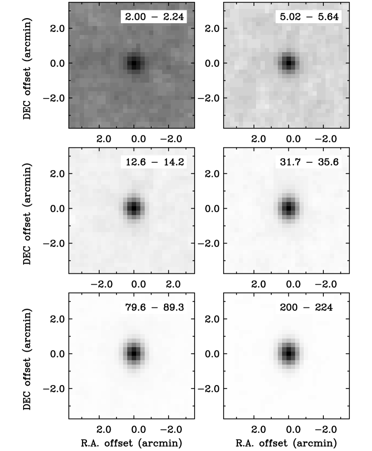
Stacked images in total intensity and polarized intensity were constructed by taking the median over all remaining postage stamps for each pixel. When we discuss the median fractional polarization from stacking, we use the ratio of the median to the median of for narrow ranges of . Figure 1 shows a sequence of stacked polarized intensity images for selected flux density ranges starting with the faintest flux density, increasing by a factor 2.5 in each step. Significant polarized emission is visible in the center of each image, increasing in strength as the median total flux density increases. The angular diameter of sources in the stacked Stokes I images is with standard deviation , consistent with the beam size of the images made by Taylor et al. (2009).
The background in the images is positive, representing the polarization bias in the absence of signal. The median of the Rice distribution in the absence of signal and noise of 0.29 mJy beam-1 is 0.3415 mJy beam-1. The actual background level is closer to 0.365 mJy beam-1, because the noise level in the NVSS Q and U images is not uniform, and possibly because of non-Gaussian wings of the noise distribution. We tested improvement of the noise with sample size by stacking randomly selected positions. Figure 2 shows the rms around the mean offset level in stacked polarized intensity images at random positions. For the rms fluctuations follow the relation . At higher , the noise in the stacked polarized intensity images decreases at a slower rate. The noise level at the break is close to the expected confusion noise level in polarization for a median percentage polarization of . While polarized sources at the confusion limit blend together and partially depolarize, the stacked image remains crowded with sources with a density of the sky that corresponds with a few beams per source. For our stacking result, we have no concern regarding confusion in polarization because the reference catalogue of NVSS sources remains well above the confusion limit. The faintest flux density bin in our analysis contains sources yielding a sensitivity of 1 Jy in the stacked image.
2.3. Polarization bias correction
2.3.1 Bias in stacked polarized intensity
Noise in polarized intensity biases the observed polarized intensity upward from the actual polarized intensity . If the signal to noise ratio is low, the relation between and the expectation value of , or the median value , deviates most strongly from a linear relation. Following Simmons & Stewart (1985), the probability density function of the polarized intensity for a source with true polarized intensity and the same but statistically independent Gaussian noise in the Stokes parameters and is the Rice distribution (Rice, 1945; Vinokur, 1965)
| (1) |
with the zeroth order Bessel function, and the unit for imaginary numbers. Consider a number of independent measurements with the same . This is not a realistic assumption in many stacking experiments, but it provides a helpful analytic expression and may proof to have a useful application in stacking polarized intensity for a number of subsequent frequency channels for the same source. The median is defined by the relation
| (2) |
In the limit of low signal to noise ratio in polarization (), we approximate the Bessel function by a polynomial approximation to second order for (Millane & Eads, 2003). Substituting this approximation in Equation 2 yields an equation for the median in the case that . Expressed in the normalized variables , , this equation is
| (3) |
For we find the exact solution for the median polarized intensity in the absence of signal, ,
| (4) |
where is the natural logarithm. For , Equation 3 gives an approximation for that deteriorates for higher values of . Substituting in Equation 2, and approximating
| (5) |
solving for yields
| (6) |
Figure 3 shows this approximate formula in comparison with the result of numerically integrating Equation 2. It is to be expected that the approximation deteriorates for larger . The difference remains within the statistical errors for samples with , for which the noise in the stacked image is more than . We will see later that a larger source of error is related to the fact that a real sample of sources contains a distribution of that is not known a priori. The dotted line in Figure 3 is the line . Its deviation from the curves illustrates that the signal in the stacked polarized intensity image is far from an addition of the source signal and the off-source median. Inverting Equation 6, we obtain an estimator for the bias correction for the median polarized intensity, assuming all sources have the same ,
| (7) |
The non-linear dependence of on the true signal is evident in Equation 6. When stacking a set of sources with different values of , sources with higher contribute more strongly to raising the median of the sample. A significant range in is to be expected when stacking a sample of sources. Considering the additional complication that the noise in a survey may not be uniform, we expect that an analytical solution as derived above leaves systematic errors that will be larger than the statistical uncertainty in the median polarized intensity of a large sample of sources.
We apply Monte Carlo simulations to derive a median from the median of the stack . Consider the stack as a sequence of observed polarized intensities , from sources with true polarized intensity (). The are realizations of a single experiment of adding noise in Stokes and , and then constructing for each source. The local noise level at each source in the stack is recorded, and the effect of the noise on the can be simulated by a large number of Monte-Carlo realizations of the stack. The most likely value for and its errors are derived from these Monte Carlo simulations.

A significant complication is that we cannot assume that all sources in a stack have the same . The expectation value or the median of the observed signals is a non-linear function of the actual signals (Figure 3 and Equation 6). The result of this non-linearity is that sources with higher in a survey with uniform noise are more effective raising than sources with low . The result of the stack therefore depends on the shape of the distribution of values, not just the median .
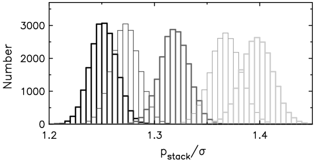
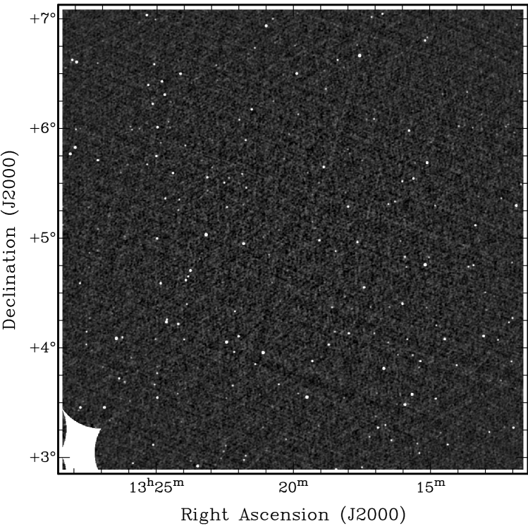
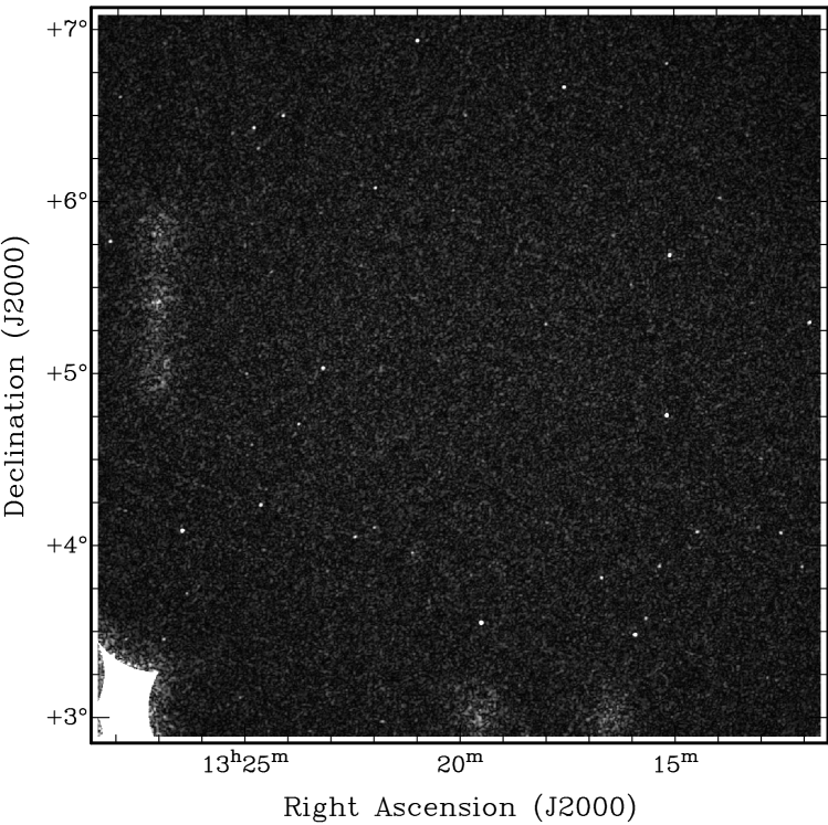
Figure 4 demonstrates the effect of different distributions with the same median . We simulated stacking of five samples of 5000 sources and uniform Gaussian noise in Stokes and with standard deviation . We note that our analysis below takes into account variation of the noise and the actual noise statistics of the survey that may or may not be Gaussian. The median polarized intensity of each simulation was the same at , but the distribution of the was different for each sample: all sources the same , a uniform distribution between and a maximum , a Gaussian distribution, a Gauss-Hermite function (van der Marel, 1993) with extended tail (kurtosis parameter , where for a Gaussian), and the distribution of for bright NVSS sources derived by Beck & Gaensler (2004). The latter is a piecewise fit to the fractional polarization distribution for NVSS sources brighter than 80 mJy. In addition, a fraction of sources is considered unpolarized. In this example, that fraction is zero. Beck & Gaensler (2004) adopted 11.3%. Each distribution was stacked in 2000 independent realizations in order to derive the distribution of the median-stacked polarized intensity . The resulting distributions of are shown in Figure 4. The total polarization bias in each stack is the difference between the median of each of the distributions shown and the intrinsic median .
Although the differences between the distributions in Figure 4 are small compared with the total bias, they are significant compared with the width of each of the distributions, which is of the order of , with in this example. In order to take optimal advantage of the increased sensitivity in the stacked images, our bias correction must include the distribution of the . This is a higher-order correction to the derived median that to some degree depends on the signal to noise ratio per object. We will include a constraint to the shape of the distribution in our analysis below. It is worth noting that for small samples, , the differences between the histograms become similar to the statistical error . For these small samples, one can apply Equation 7 as a bias estimator. The implied delta function distribution tends to underestimate for a given compared with distributions of finite width, so this estimator is biased toward higher for a given .
2.3.2 Bias correction of stacked polarized intensity
When stacking sources selected in a narrow range of total intensity, the distribution of is of the same form as the distribution of fractional polarization , which is at best slowly varying with flux density as the relative numbers of radio source populations change gradually with flux density. The distribution derived for bright sources can be used as an initial estimate for the distribution if the sources span a narrow range in total flux density. Note that this solution works well for samples that can be binned by their Stokes I flux density. When stacking targets selected at a different wavelength, such as a different radio frequency, X-ray, or optical source catalogue, an a-priori estimate for the distribution of the is much more complicated.
In order to proceed, an additional constraint for the distribution of the is required. When we refer to a fixed shape of the distribution, we still allow for a scaling in that changes the median. While this is an approximation, it allows us to use prior information from brighter sources as a basis for our analysis. A constraint for the shape of the distribution is available if the number of sources is sufficiently large. The distribution of the observed values contains information about the distribution of the , even though it is broadened by the effects of noise. Our Monte Carlo simulations reproduce the effect of the noise in polarized intensity for a proposed distribution of . The distribution of the synthesized polarized intensities including noise can be compared with the distribution of observed . The metric by which we decide whether the assumed distribution of is acceptable, is the ratio of the upper quartile to the lower quartile of the distribution of the observed . This ratio is still fairly robust against outliers, which is necessary when stacking real data.
For sources selected in a narrow range of total intensity, the shape of the distribution of observed approaches the distribution in the limit of high signal to noise ratio, while it approaches the distribution of the noise in the limit of no polarized signal. In between these two limiting cases, we find a transition between the two distributions that occurs over an order of magnitude in or more. The ratio of the upper quartile to the lower quartile of the observed values of the sources in the stack is sensitive to the shape of this distribution, but not to the median itself. It therefore provides an additional constraint to the shape of the distribution that is not sensitive to outliers, provided is sufficiently large.
Polarization bias correction proceeds as follows. For each source in the stack, we draw a and polarization angle, and noise perturbations to simulate observed and (). The resulting set of polarized intensities is stacked, retrieving and quartiles. Repeat this times to define the distribution of for the input parameters. This procedure must be repeated for a sequence of assumed median values and distributions of until the quartile ratio matches that of the data in the stack for every flux density bin. The input parameters vary little from one flux bin to another, allowing targeted search ranges for these parameters to be defined. Retrieving the distribution from the observed distribution is a deconvolution problem that can in principle be solved separately, with the result feeding back into the stacking analysis. This may be necessary if one finds that the distribution derived from bright sources does not reproduce the quartile ratio derived from the data at lower flux densities. The signal to noise ratio for which any particular shape can be confidently rejected or accepted in this way depends on the size of the samples. While a complete analysis of all possible shape distribitions is beyond the scope of this paper, we illustrate this further in the following sections.
2.4. A stacking simulation

In order to test the stacking and bias correction, simulated images such as the one shown in Figure 5 were made, that contain image artifacts and spatial variation of the noise similar to that encountered in NVSS images. Total flux densities in the range 0.1 mJy to 1 Jy were drawn from a power law distribution. The percentage polarization of each source is drawn from a distribution fitted to NVSS sources brighter than 80 mJy by Beck & Gaensler (2004). The inserted median is independent of flux density. Each source is assigned an arbitrary polarization angle, dividing the polarized signal over Stokes and . To simulate imperfect imaging each source is added to the simulated image in a way that mimics interferometric imaging with a finite clean limit of mJy beam-1 and a Gaussian restoring beam. Residual side lobes are appropriately scaled VLA-D antenna patterns centered on the location of the source. These side lobes add incoherently, creating a non-Gaussian noise floor after which Gaussian noise modulated by the sensitivity pattern of NVSS mosaics is added. We included some weight patterns of incomplete mosaics that lead to variation in the noise level around missing fields.
We stacked polarized intensity following the procedure outlined above. The results are shown in Figure 6 and Figure 7. Each point in Figure 6 represents a stack with its own Monte Carlo analysis. Note that the formal errors in the median fractional polarization in Figure 6 are smallest in the central part of the flux density range, and larger for brighter sources and for fainter sources. Errors are larger for brighter sources because the sample sizes are smaller, while for fainter sources the signal to noise ratio in the stacked image decreases as the signal gets weaker, despite the larger sample size. The input median fractional polarization is recovered within the errors over the entire flux density range shown. To illustrate the magnitude of the bias correction in the fainter bins, the ratio is shown by the gray curve. The dotted curve shows the result of Monte Carlo simulations that assume a Gaussian distribution of , which is rejected because it does not reproduce the shape of the distribution of the at intermediate flux densities as explained below.
Figure 7 shows the ratio of the upper to the lower quartile of the set of for each of the stacks as a function of flux density (points with error bars), along with a curve that shows the mean quartile ratio of the 2000 Monte-Carlo simulations for each stack. The shape of the curve illustrates the transition from the noise dominated regime to the signal dominated regime. The zero-signal stack reproduces the off-source values in the stacked image. Recall that for sources fainter than mJy in the NVSS, more than 50% of the sources is no longer formally detectable, leaving the median undetermined unless stacking is attempted. This analysis cannot provide a unique shape for the distribution of , but it is sufficiently sensitive in the transition region to differentiate between a Gaussian distribution and the actual non-Gaussian shape of the distribution of NVSS sources. The dotted curve in Figure 7 shows the quartile ratio for the Monte Carlo simulations that assumed a Gaussian distribution. A Gaussian distribution is rejected for sources with , while the distribution for bright sources consistently reproduces the quartile ratio over the entire flux density range. Note that we have to assume that the shape of the distribution does not change for sources fainter than 10 mJy. However, we do not expect the shape of the distribution to change rapidly with flux density.
2.5. Results from stacking NVSS polarized intensity


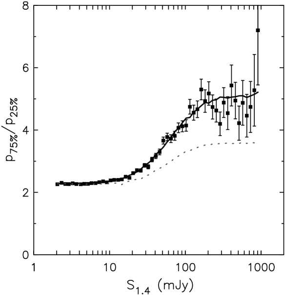
For stacking NVSS sources, we used the distribution fitted by Beck & Gaensler (2004), with 6% of sources completely unpolarized. The median fractional polarization of NVSS sources as a function of flux density is shown in Figure 8, and the accompanying quartile ratio in Figure 9. We find the median fractional polarization is higher for fainter radio sources. The line in Figure 8 represents the fit
| (8) |
where is expressed as percent polarization, and is the 1.4 GHz flux density in mJy. We see small systematic residuals around this best fit line. While this may indicate real curvature in the relation, it may also indicate resolution effects for bright sources that are difficult to quantify. On one side, slightly resolved sources may be more highly polarized because structure in polarization angle leads to depolarization in an unresolved source. On the other side, the stacking centers at the peak of total intensity, and may miss polarized components that are offset from the peak in total intensity. A second degree polynomial fit to the data has a maximum fractional polarization of 2.4% at flux density , with considerable uncertainty. We apply the linear fit above for our derivation of polarized source counts below, but include the second order fit in our error analysis.
Figure 9 shows the quartile ratio as a function of flux density for the same stacks. The dashed curve shows the quartile ratio for Monte Carlo simulations of the stack that included noise only, while the solid curve also included residual instrumental polarization, modeled as a random term in and that is Gaussian with standard deviation of Stokes I, similar to the expected residual leakage in the NVSS. Despite extensive modeling, including residual leakage was required to fit the quartile ratio over the full flux density range considered. The NVSS stacking results presented here account for this leakage term, but we note that the result in Figure 8 is not sensitive to this detail because the median is substantially larger than the residual instrumental polarization after calibration. In a future paper we will present a sample of flat spectrum sources stacked in the same way with median below , independent of flux density. In that case, it is more important to account for residual instrumental polarization.
3. Polarized radio source counts
| (mJy) | ||
|---|---|---|
| 0.0050 | 0.0103 | |
| 0.0083 | 0.0133 | |
| 0.0138 | 0.0175 | |
| 0.0229 | 0.0241 | |
| 0.0380 | 0.0340 | |
| 0.0631 | 0.0489 | |
| 0.1047 | 0.0706 | |
| 0.1738 | 0.1027 | |
| 0.2884 | 0.1503 | |
| 0.4786 | 0.2217 | |
| 0.7943 | 0.3295 | |
| 1.318 | 0.4828 | |
| 2.188 | 0.6814 | |
| 3.630 | 0.9115 | |
| 6.026 | 1.135 | |
| 10.00 | 1.320 | |
| 16.60 | 1.454 | |
| 27.54 | 1.572 | |
| 45.71 | 1.690 | |
| 75.86 | 1.626 | |
| 125.89 | 1.235 | |
| 208.93 | 0.724 | |
| 346.74 | 0.283 |
Equation 8 can be combined with radio source counts in total intensity to predict polarized radio source counts in a similar fashion as Beck & Gaensler (2004). Stacking allows us to probe the fractional polarization of radio sources more than an order of magnitude deeper than previous work based on the NVSS, probing the flux density range where most AGN in the radio source counts have radio luminosity below the traditional FRI/FRII luminosity boundary (e.g. Wilman et al., 2008).
We combine the stacking results with total intensity source counts from the SKADS S3 simulation of Wilman et al. (2008). These model source counts fit observed radio source counts well, except maybe at the very bright end which is less important for our purpose. The models also provide a physically motivated extrapolation to lower flux densities. We used all sources of type AGN, adding the fluxes of multiple components where appropriate. For the flux range that we consider here, these Stokes I source counts consist of FR I and FR II class sources with a minor contribution of radio-quiet QSOs at the faint end of the flux density range considered here.
Equation 8 is a fit to data for sources with flux density . A median percentage polarization of corresponds to a median polarized flux density of . For polarized flux densities , the polarized source counts are therefore directly constrained by stacking. Below this flux density, our tabulated polarized source counts represent an extrapolation of Equation 8. We do not expect a sudden change in polarization properties of radio sources at any flux density, because radio sources at any flux density include sources with a wide range in luminosity and red shift. This ”convolution with the universe” justifies extrapolation by a factor in flux density. The polarized source counts we derive in this flux density range will not be seriously affected by an emerging polarized source population at the faint end.
Table 1 lists Euclidean-normalized differential source counts and cumulative source counts derived by convolving the AGN total-intensity source counts from Wilman et al. (2008) with the distribution of derived from stacking. These models provide us with an AGN-only version of radio source counts that matches the population of radio sources stacked. For the purpose of this paper, it is sufficient that these models fit observed source counts in the flux density range of interest, while the cosmological details may only affect the results insofar they rely on separation of different populations of radio sources.
The uncertainty in the polarized source counts is a result of uncertainty in the AGN source counts from the Wilman et al. (2008) simulation, and uncertainties in the results from stacking. In the flux density range (2 mJy - 30 mJy), the median fractional polarization is directly constrained by stacking, and the AGN component of the source counts in the SKADS S3 simulations is well-constrained by observations. According to the models, these AGN are dominated by radio sources with luminosity consistent with type FR I. Below mJy, the total source counts are increasingly dominated by star forming galaxies, and observed source counts from small deep fields show considerable spread. While a significant fraction of radio sources with 1.4 GHz flux density in the range 0.1 - 1 mJy is AGN related (Gruppioni et al., 1999), the AGN fraction below 1 mJy becomes gradually more uncertain, introducing uncertainty that grows with the degree of extrapolation to lower flux densities. The radio-quiet QSO population in the models represents objects in the low-luminosity end of the radio luminosity function of AGN that are not well represented in the flux density range of NVSS sources. Within the context of the Wilman et al. (2008) models, it appears reasonable to extrapolate the stacking results over about an of magnitude in flux density below the faintest flux density bin that was actually stacked. We therefore apply , or as the limits for the polarized source counts, while noting that the stacking experiment constrains these counts directly for .
Formal errors in the fit given in Equation 8 result in an uncertainty on the level of a few percent in the cumulative source counts at in Table 1. We estimate the actual errors in the normalization of the fit to be closer to 5% - 10% considering variation associated with the uncertainty in the distribution of . If we apply a second-order polynomial fit, the cumulative polarized source counts for are 10% lower than listed in Table 1. For comparison, the cumulative counts at 5 Jy would be 30% lower than listed in Table 1 if the median fractional polarization is held constant at 2%.
4. Discussion
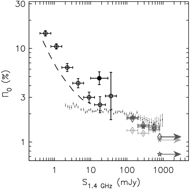
Figure 10 compares published median as a function of flux density with the results of this paper. The main source of data for is the NVSS (Condon et al., 1998), with sample sizes for individual flux ranges. Data for fainter sources come from various deep observations of small fields that detected in order of sources in polarization.
The data in Figure 10 show a tendency for higher fractional polarization in faint sources. Closer inspection reveals some notable differences between the published values. At flux densities higher than 100 mJy, the difference in fractional polarization between flat spectrum sources and steep spectrum sources noted by Mesa et al. (2002) and Tucci et al. (2004) is clearly visible. It is not surprising that our results agree with their steep spectrum sources, since a large majority of radio sources has a steep spectrum. A paper presenting stacking polarized intensity for samples selected by spectral index is in preparation. The stacking results presented here are slightly above the medians for steep spectrum sources reported by these authors, with medians that are higher, approximately the formal error per data point in the stacking experiment. The results of Mesa et al. (2002) and Tucci et al. (2004) differ mutually by a similar amount, with slightly higher values reported in Tucci et al. (2004). The NVSS catalogue is strictly speaking a catalogue of source components, and the differences between Mesa et al. (2002) and Tucci et al. (2004) can be ascribed to differences in source selection (see Tucci et al., 2004, for a discussion). The latitude cut-off appears too close to the Galactic plane since the NVSS has been shown to suffer from localized bandwidth depolarization up to latitudes (Stil & Taylor, 2007). Experiments with different latitude cut-offs on the entire NVSS catalogue suggest that the median fractional polarization varies on the level of depending on the choice of the latitude cut-off. Mesa et al. (2002) also found a median fractional polarization of 2.2% for all NVSS sources brighter than 80 mJy, which is in good agreement with the results from stacking. While a small systematic difference exists, we recall that the stacking result is based on NVSS images at resolution made by Taylor et al. (2009), and that the latitude cut-off and the correction for polarization bias are different.
The differences with the literature are larger for sources fainter than at 1.4 GHz. The surveys below mJy are different in observational setup, and the results have been derived using different methods. While it is possible that cosmic variance may cause differences between the results of small fields, we suspect that differences in survey parameters (mean signal to noise ratio at a given polarized flux density, resolution) and details of source detection and treatment of polarization bias contribute considerably to the differences between surveys.
The median reported by Taylor et al. (2007) is the highest value between 10 mJy and 100 mJy, approximately higher than the results of Subrahmanyan et al. (2010) and the values from the present stacking analysis in the same flux density range. The survey areas, angular resolution, and sensitivity of the surveys of Taylor et al. (2007) and Subrahmanyan et al. (2010) are comparable. Macquart et al. (2012) found a mean fractional polarization of 3.7% for sources below 20 mJy in the Centaurus field, not shown alongside the medians in Figure 10. These authors also list 3% polarization for sources brighter than 200 mJy, which is substantially higher than the median of NVSS sources, because it represents a mean, not a median. If the ratio of mean to median for bright sources can be applied to faint sources, the median for faint sources in the Centaurus field would be , in the range of from the ATLBS survey and the present analysis around . Macquart et al. (2012) fitted a broken power law to the observed distribution of polarized intensities without the need of a bias correction. Although their data can be fitted with a significant change in slope of the polarized source counts, the authors summarized their result as no turnover above 0.2 mJy.
Before we discuss the higher value from Taylor et al. (2007) in this context, we examine the data for sources fainter than 10 mJy. Below 10 mJy, the medians reported by Subrahmanyan et al. (2010) show a sharp rise toward lower flux density, while the stacking experiment presented here shows a much more gentle increase.
The sharp rise in median fractional polarization found by Subrahmanyan et al. (2010) is a result of their polarization bias correction. Subrahmanyan et al. (2010) applied a polarization bias correction of the form . The factor corrects for the size of the aperture in which and were integrated, and it accounts for correlation of pixel values on small angular scales arising from convolution with the synthesized beam. We illustrate the problem with a simulation, represented by the dashed curve in Figure 10. Sources were drawn from the source counts curve of Hopkins et al. (2003), and assigned a drawn from the distribution used in our stacking analysis with (Equation 8 for ), independent of flux density. For a random position angle, Gaussian noise with standard deviation mJy beam-1 was added to the simulated Stokes and . The factor is difficult to model. It is equivalent to say that the noise in the integrated and flux density is a factor higher than for single-pixel values, and use this higher noise value in the conventional bias correction . By using only the central noise value mJy beam-1, we implicitly assume for every source and also a constant noise level in the ATLBS mosaic. This means that the simulation adds less noise than it should for some sources. As a result, our simulation does not include some of the more biased sources in the sample.
The standard polarization bias correction is applied to each source. If the bias-corrected polarized flux density is assigned the value zero. The resulting median fractional polarization as a function of flux density is represented by the dashed curve in Figure 10, which resembles the steep rise found by Subrahmanyan et al. (2010), even though the true median is constant at 2.44%. The simulation results remain below the data of Subrahmanyan et al. (2010), but this is at least in part because the actual noise for some sources must be higher than the minimum noise used in the simulation. The dashed curve in Figure 10 is not very sensitive to the assumed slope of the Stokes source counts on the faint end. Repeating the simulation with a power law with slope to fitted to the actual counts listed by Subrahmanyan et al. (2010) gave the same results. Setting the slope of the Stokes source counts to zero results in a slightly lower curve, approximately , indicating a minor contribution of the Eddington bias (Eddington, 1913; Teerikorpi, 2004).
We conclude that the main reason for the high fractional polarization reported by Subrahmanyan et al. (2010) is the application of an incorrect bias correction for sources with a low signal to noise ratio. Their estimator for has a bimodal distribution for faint sources, with a peak at zero arising from sources with , and a broader peak around . For faint sources, the relative error in the estimator of is large and asymmetric (e.g. Vaillancourt, 2006).
The forward fitting of polarized source counts by Macquart et al. (2012) avoids a correction for polarization bias and naturally accounts for Eddington bias. These authors warned against considering only the mean bias correction for analysis. Macquart et al. (2012) fitted a double power law model of the polarized source counts to the observed distribution of . The model source counts are formulated in terms of . Interpretation of the result is complicated for a survey with non-uniform noise. The percentage polarization is derived by inverting the polarized source counts to the total-intensity source counts. This requires an assumption of the shape of the distribution. Our procedure for stacking polarized intensity includes variation of the noise, and constrains the distribution of to the extent possible. Macquart et al. (2012) work with results derived from Faraday Synthesis (Brentjens & de Bruyn, 2005), where the present analysis is strictly speaking applicable to narrow-band observations. Specific applications of stacking to wide-band polarization surveys are discussed briefly in Section 4.2.
The Monte-Carlo simulations in Taylor et al. (2007) included varying noise across the mosaic and the slope of the radio source counts in order to correct for these effects. The cause of the discrepancy between the present result and the higher median from Taylor et al. (2007) is therefore not immediately clear. The median fractional polarization derived by these authors, compared with the polarization of detected sources with flux density near 10 mJy, indicates that the detected sources are well in the tail of the distribution, at 2 to 4 times the median. The median fractional polarization in this case may depend on the adopted slope of the source counts because both can affect the number of faint sources with polarized flux density higher than the median. Experiments at the time did not suggest a strong dependance of the result on the adopted shape of the source counts or the detection threshold. A more likely potential cause for a higher median resulting from the analysis of Taylor et al. (2007) is a more implicit effect related to the Eddington bias mentioned above. Although the Monte Carlo simulations in Taylor et al. (2007) were designed to account for such bias, the likelihood function in their Equation 6 contains only the error in associated with the noise in the image at the position of the source. While the simulated distributions in and did include the effect of noise, the detection threshold and implicitly the Eddington bias through the use of the source counts curve in the simulations, sources with high but low due to their position in the mosaic may have received disproportionate weight in the likelihood function, because the error bars derived from the noise in the images would not accurately reflect the width of the probability distribution of for those sources. This may have lead the maximum likelihood fit to a higher median. A re-analysis of the more sensitive ELAIS N1 data from Grant et al. (2010) is required to verify this suggestion.
With stacking we measured the median fractional polarization over nearly 3 orders of magnitude in flux density. The results are mostly consistent with previous studies of the NVSS above 80 mJy, and the trend for higher fractional polarization we find down to appears to be an extension of the trend seen for brighter sources by Mesa et al. (2002) and Tucci et al. (2004). The increase in fractional polarization is so gradual that it becomes comparable to the statistical errors for a modest sample size of order 100 per flux density bin, that may be obtained from a deep integration of a small area of the sky. While we find consistency with deep-field results in their high signal to noise ratio limit, the median fractional polarization derived here is on the low side of the range of published values for sources fainter than 100 mJy. This illustrates how stacking can supplement observations of small areas with high sensitivity.
Establishing the trend in polarization with flux density of AGN provides an extra constraint that allows us to include magnetic field properties in models of the cosmic evolution of radio sources through radio source counts. The cause of the gradual change in with flux density is not known. We speculate that this gradual change is related to a gradual shift in the radio source population, for example between steep and flat spectrum sources. Stacking as a function of spectral index will be the subject of a subsequent paper.
4.1. Density of the RM grid
A key parameter for the scientific impact of all-sky polarization surveys is the density on the sky of lines of sight with a measured rotation measure (the RM grid). The polarized source counts presented here are on the low side of the range considered by Stepanov et al. (2008), but they agree well with a recent determination by Rudnick & Owen (2014). Macquart et al. (2012) sound a slope for the differential polarized source counts by fitting a power law count to polarized intensity distribution of sources not formally detected, comparable to the slope they found for detected sources in the range . The slope of the differential source counts in Table 1 is between and , and between and . The effect of the increase in fractional polarization is in part compensated by a gradual decrease in the slope of the total intensity source counts of the same radio sources.
The Polarization Sky Survey of the Universe’s Magnetism (POSSUM, Gaensler et al., 2010) is designed with a target sensitivity of . Rotation measures can be extracted for sources with signal to noise ratio in polarization or . The results in Table 1 suggest POSSUM will detect approximately 26 polarized sources per square degree extragalactic sky, and fewer close to the Galactic plane where confusion with the diffuse Galactic foreground will likely reduce completeness. If each detected polarized source above the threshold yields a useful RM measurement, the mean angular distance between RMs will be about . The RM catalogue from Taylor et al. (2009) contains approximately one source per square degree.
Beck & Gaensler (2004) assumed in their analysis that only 50% of polarized sources provide useful RMs. When comparing the present results with their extrapolated source counts this factor 2 must be taken into account. The present polarized source counts at are then a factor 2 lower than those of Beck & Gaensler (2004), even though we find a gradual increase in fractional polarization for fainter sources. The difference is in the adopted total-intensity source counts. Beck & Gaensler (2004) used the total source counts from Hopkins et al. (2003) that include a change of slope below 1 mJy that is generally attributed to star forming galaxies. The polarized source counts presented here are AGN-only counts. Spiral galaxies may contribute to polarized source counts at 1.4 GHz, although depolarization is strong at 1.4 GHz (Stil et al., 2009; Sun & Reich, 2012). Polarized source counts models by Stil (2009a) show a significant contribution by spiral galaxies to the total polarized source counts below , but these models did not yet take into account an anti-correlation between fractional polarization and luminosity reported by Stil et al. (2009).
In summary, the lower fractional polarization we find in this paper lead to a downward revision of the expected density of the RM grid from sky surveys with Jy sensitivity by a factor of a few. A recent paper on polarization in the GOODS-N field by Rudnick & Owen (2014) comes to a similar conclusion. There is some latitude in the assumption that only 50% of sources may yield useful RMs. For faint sources, statistical errors will dominate over complexity of the sources. What constitutes a useful RM may differ between applications.
4.2. Channel stacking of polarized intensity
Future surveys of polarized radio emission will yield spectral image cubes of the Stokes parameters that provide the sensitivity of broad bandwidth but avoid bandpass depolarization. Rotation Measure synthesis (Brentjens & de Bruyn, 2005) is the preferred method to derive polarization properties of radio sources from these spectropolarimetric surveys. The detection threshold for Faraday synthesis for a predetermined acceptable false detection rate is higher because of the unknown rotation measure of a source (George et al., 2012; Macquart et al., 2012). The detection threshold depends on the Faraday depth range that is searched.
The improvement of the noise level we found in the NVSS up to sample size in principle provides sufficient sensitivity to detect polarization for samples selected at other wavelengths that remain below the detection threshold in total flux density. The number of targets is typically much larger than the number of frequency channels, which will be of order for surveys with bandwidth of 1 GHz and frequency channels of 1 MHz. The expected sensitivity for stacking a sample of in a single frequency channel of a wide-band polarization survey is therefore an order of magnitude larger than the expected sensitivity for a single source employing the full bandwidth. The advantage of high sensitivity in a narrow frequency range is that it allows investigation of the fractional polarization as a function of redshift in the rest frame of the target sample, using the bandwidth of the survey to trace the same emitting wavelength over a signifcant range in cosmological redshift. This becomes significant for surveys with the SKA, that will provide large samples of sources at a wide range of redshifts. Stacking polarized intensity can thus supplement Faraday synthesis in investigations of the polarization of radio sources over cosmic time, as it capitalizes on a unique slice in multi-dimensional data space. The stacking experiment itself can address some aspects of Faraday rotation in the source if one stacks the sample not just in individual channels, but also in channel averages of polarized intensity, taking both the vector sum and the scalar sum of polarized intensity over adjacent channels across the band.
Stacking (averaging) polarized intensity per channel in principle can detect polarization of fainter sources than rotation measure synthesis with a high significance level. A difference with the stacking discussed in this paper is that one can use the mean polarized intensity in place of the median intensity, because extreme data values are not expected. The central limit theorem applies and provides an analytic expression for the distribution of the outcome of the stack, provided that polarized intensity, or more precisely the signal to noise ratio in polarized intensity, is trusted to be constant across the frequency band. If the median is used, the bias correction in Equation 7 can be applied to this problem. If the polarized intensity is not constant, the non-linear relation between and introduces similar challenges as described in this paper for stacking polarized intensity from different sources. Polarized intensity is likely to change between channels in surveys with a large bandwidth because its frequency dependence is the same as total intensity if the fractional polarization is constant, and because the system temperature may not be constant over the observed frequency range. If the polarized emission in a source is the composite of two or more regions subject to different amounts of Faraday rotation, the vector sum of different RM components can also lead to complicated variation of polarized intensity with frequency.
Spectral index effects can be removed by dividing polarized intensity by total intensity. The statistics of the ratio is not strictly Ricean because and will not have Gaussian statistics, even if the noise in , , and is Gaussian. If the signal to noise ratio in in a single frequency channel is high, Ricean statistics may apply, and a correction can be made for polarization bias similar to that described in Section 2.3.2 with Monte-Carlo simulations, or based on the central limit theorem. If significant variation in exists, it will be difficult to extract even a mean or median value because the distribution of intrinsic values must be taken into account. Splitting up the frequency band into a small number of sub-bands and stacking each sub-band individually can reduce this problem, or make it apparent that a more detailed analysis is required. If the noise is not uniform across the frequency band, one also needs to model the range of signal to noise ratios in the data. Failing to do so may lead to systematic errors as a function of signal to noise ratio.
5. Conclusions
Stacking polarized intensity allows us to investigate the faint polarized signal of radio sources, using large samples covered by wide-area radio surveys. This technique is already useful at higher flux densities where a significant fraction of sources is detectable in polarization. As the sample covers a large area of the sky, results from stacking are not sensitive to cosmic variance. It opens the possibility to investigate the polarization of sources with a low density on the sky, for which narrow deep fields do not provide a large enough sample.
We present a procedure for stacking polarized intensity that uses the shape of the distribution of data values going into the stack as an additional constraint to solve for the unknown intrinsic distribution of polarized intensity of the sample.
We find that the median fractional polarization of sources detected by the NVSS from stacking polarized intensity is higher for fainter sources, but the degree of polarization of sources in the flux density range 2 to 20 mJy remains below 2.5%, which is significantly smaller than claimed by previous work. Polarized radio source counts for radio sources powered by an active galactic nucleus are derived from stacking by convolving the distribution with total-intensity counts modeled by Wilman et al. (2008). These new source counts for are on the low side of the spectrum of predictions made for the design of future polarization surveys with the SKA and its path finders, ASKAP and MeerKAT.
Acknowledgments
This research has been made possible by a Discovery Grant from the Natural Sciences and Engineering council of Canada to Jeroen Stil. JMS thanks L. Rudnick and the anonymous referee for their comments on the manuscript. The National Radio Astronomy Observatory is a facility of the National Science Foundation operated under cooperative agreement by Associated Universities, Inc.
References
- Beck & Gaensler (2004) Beck, R. and Gaensler, B. M. 2004, Observations of magnetic fields in the Milky Way and in nearby galaxies with a Square Kilometre Array, in New Astronomy Reviews, 48, 1289
- Brentjens & de Bruyn (2005) Brentjens, M. A., & de Bruyn, A. G. 2005, A&A 441, 1217
- Condon et al. (1998) Condon, J. J., Cotton, W. D., Greisen, E. W., et al. 1998, AJ, 115, 1693
- Eddington (1913) Eddington, A. S. 1913, MNRAS, 73, 359
- Gaensler et al. (2010) Gaensler, B., Landecker, T., & Taylor, A. R. 2010, BAAS, 42, 515
- Garn & Alexander (2009) Garn, T., & Alexander, P. 2009, MNRAS, 394, 105
- George et al. (2012) George, S. J., Stil, J. M., & Keller, B. W. 2011, PASA, 29, 214
- Grant et al. (2010) Grant, J. K., Taylor, A. R., Stil, J. M., et al. 2010, ApJ, 714, 1689
- Gruppioni et al. (1999) Gruppioni, C., Mignoli, M., & Zamorani, G. 1999, MNRAS, 304, 199
- Hopkins et al. (2003) Hopkins, A. M., Afonso, J., Chan, B., et al. 2003, AJ, 125, 465
- Jarvis et al. (2010) Jarvis, M. J., Smith, D. J. B., Bonfield, D. G., et al. 2010, MNRAS, 409, 92
- Macquart et al. (2012) Macquart, J.-P., Ekers, R. D., Feain, I., & Johnston-Hollitt, M. 2012, ApJ, 750, 139
- Mesa et al. (2002) Mesa, D., Baccigalupi, C., De Zotti, G., et al. 2002, A&A, 396, 463
- Millane & Eads (2003) Millane, R. P., & Eads, J. L. 2003, IEEE Transactions on Antennas and Propagation, 51, 1398
- O’Sullivan et al. (2008) O’Sullivan, S., Stil, J. M., Taylor, A. R., et al. 2008, in Proceedings of the 9th European VLBI Network Symposium on The role of VLBI in the Golden Age for Radio Astronomy and EVN Users Meeting, PoS(IX EVN Symposium)107
- Rice (1945) Rice, S. O. 1945, Bell Syst. Tech. J., 24, 46
- Rudnick & Brown (2009) Rudnick, L., & Brown, S., 2009, AJ, 137, 145
- Rudnick & Owen (2014) Rudnick, L., & Owen, F. N. 2014, ApJ, in press arXiv:1402.3637
- Sadler et al. (2006) Sadler, E. M., Ricci, R., Ekers, R. D. et al. 2006, MNRAS, 371, 898
- Simmons & Stewart (1985) Simmons, J. F. L., & Stewart, B. G. 1985, A&A, 142, 100
- Stil & Taylor (2007) Stil, J. M., & Taylor, A. R. 2007, ApJ, 663, L21
- Stil et al. (2009) Stil, J. M., Krause, M., Beck, R., & Taylor, A. R. 2009, ApJ, 693, 1392
- Stil (2009a) Stil, J. M. 2009a, in The Low-Frequency Radio Universe, in ASP Conf Ser. 407, Eds Saikia, Green, Gupta, & Venturi San Francisco:ASP, 147
- Stepanov et al. (2008) Stepanov, R., Arshakian, T. G., Beck, R., Frick, P., & Krause, M. 2008, A&A, 480, 45
- Subrahmanyan et al. (2010) Subrahmanyan, R., Ekers, R. D., Saripalli, L., & Sadler, E. M. 2010, MNRAS, 402, 2792
- Sun & Reich (2012) Sun, X. H. & Reich W. 2012, A&A, 543, 127
- Taylor et al. (2007) Taylor, A. R., Stil, J. M., Grant, J. K., et al. 2007, ApJ, 666, 201
- Taylor et al. (2009) Taylor, A. R., Stil, J. M., & Sunstrum, C. 2009, ApJ, 702, 1230
- Teerikorpi (2004) Teerikorpi, P. 2004, A&A, 424, 73
- Tucci et al. (2004) Tucci, M., Martínez-González, E., Toffolatti, L., González-Nuevo, J., & De Zotti, G. 2004, MNRAS, 349, 1267
- Vaillancourt (2006) Vaillancourt, J. E. 2006, PASP, 118, 1340
- van der Marel (1993) van der Marel, R. P., & Franx, M. 1993, ApJ, 407, 525
- Vinokur (1965) Vinokur, M., 1965, Ann. d’Astrophys., 28, 41
- White et al. (2007) White, R. L., Helfand, D. J., Becker, R. H., Glikman, E. & De Vries, W. 2007, ApJ, 654, 99
- Wilman et al. (2008) Wilman, R. J., Miller, L., Jarvis, M. J., et al. 2008, MNRAS, 388, 1335