Mode propagation and attenuation in lined ducts

Abstract

Optimal impedance for each mode is an important concept in an infinitely long duct lined with uniform absorption material. However it is not valid for finite length linings. This is because that the modes in lined ducts are not power-orthogonal; the total sound power is not equal to the sum of the sound power of each mode; cross-power terms may play important roles. In this paper, we study sound propagation and attenuation in an infinite rigid duct lined with a finite length of lining impedance. The lining impedance may be axial segments and circumferentially non-uniform. We propose two new physical quantities $\mathsf{K_{p}}$ and $\mathsf{S}$ to describe the self-overlap of the left eigenfunction and right eigenfunction of one mode and the normalized overlap between modes, respectively. The two new physical quantities describe totally the mode behaviors in lined ducts.

1 Introduction

Optimal impedance is an important concept in lined ducts. It provides a theoretical limit for the maximum attenuation that can be obtained. The concept of optimal impedance was proposed firstly by Cremer[1] for the so called “least attenuation mode” (usually the plane mode). It was extended by Tester[2, 3] for any guided modes and shown to correspond to the double roots of the dispersion equation. Similar conclusion was also proposed by Shenderov[4]. However, this concept is only correct in an infinitely lined duct, which is never the case in practice.

In a lined duct, length of lining is finite, the lining impedance maybe uniform or non-uniform along axial or transverse directions. In this case, the concept of optimal impedance is not valid. This optimum impedance might not exist. A number of numerical studies were proposed to try to increase the attenuation by parameter studies[5, 6, 7, 8, 9, 10, 11]. However, to the best of our knowledge, we do not know, till now, what physical quantities play important roles in the attenuation of sound power in a practical lined duct.

Mode scattering is expected as the main mechanism to increase the attenuation. But sometimes, this scattering effects are impressive, e.g., the penalty effects of splices[10, 11, 12, 13]; others, they might be not visible[14]. We still have not a deep understanding about mode scattering, specially the liner mode scattering.

Modes in lined ducts are not orthogonal in the standard definition

$$\int_{s}\tilde{\phi}_{i}^{*}\tilde{\phi}_{j}ds=\Lambda_{i}\delta_{ij},$$ (1)

as in rigid or non-absorptive ducts where left eigenfunctions $\tilde{\phi}_{i}^{l}$ are equal to right eigenfunctions $\tilde{\phi}_{i}^{r}$, $\tilde{\phi}_{i}^{l}=\tilde{\phi}_{i}^{r}=\tilde{\phi}_{i}$, ”*” refers to complex conjugate, $\Lambda_{i}$ refers to normalization constant. When the lining impedance is absorptive, or in other words, it is complex, left eigenfunctions are not equal to right eigenfunctions. Modes are bi-orthogonal

$$\int_{s}(\tilde{\phi}_{i}^{l})^{*}\tilde{\phi}_{j}^{r}ds=\Lambda_{i}\delta_{ij}.$$ (2)

If there exist some kinds of symmetric, left eigenfunctions may be equal to the conjugate of right eigenfunctions i.e., $(\tilde{\phi}_{i}^{l})^{*}=\tilde{\phi}_{i}^{r}$. In this case, the bi-orthogonal condition is $\int_{s}\tilde{\phi}_{i}^{r}\tilde{\phi}_{j}^{r}ds=\Lambda_{i}\delta_{ij}$. When modes are not orthogonal, the total sound power is not equal to the sum of the sound power of each mode; the cross-power terms may play important roles. Therefore, although the attenuation for each mode might be maximum near the corresponding optimum impedance, the total sound power is not optimum because of the cross-power.

In this paper, we study sound propagation in a uniformly rigid duct fitted with finite length of lining without flow. We express the sound field in the lined region in terms of liner modes. We define two new physical quantities $\mathsf{K_{p}}$ and $\mathsf{S}$ to describe mode self-overlap and mutual overlap, respectively, in the lined region. We show that these two new physical quantities play essentially roles in the sound attenuation in lined region.

2 Derivation of Equations

We consider an infinite rigid duct with circular cross section lined with a region of circumferentially nonuniform liner. The liner properties are assumed to be given by a distribution of locally reacting impedance. Without significant loss of generality, the distribution may be assumed axially segmented, i.e., the impedance is set piecewise constant along the duct, while being arbitrarily variable along the circumference of each segment. In Fig. 1 the

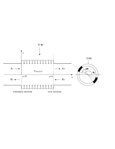
Figure 1: Configuration of one axial segment nonuniform lined duct.

configuration of one axial segment of lining impedance is depicted, the circumferential variation of impedance is presented as two acoustically rigid splices, which is a typical configuration in the intake of an aeroengine. For simplicity, we assume the circumferential nonuniformity has a mirror symmetry. Linear and lossless sound propagation in air is assumed. With time dependence $\exp(j\omega t)$ omitted, the equation of mass conservation combined with the equation of state, and the equation of momentum conservation are written as

$$\mathbf{\nabla}\cdot\mathbf{v} = -\frac{j\omega}{\rho_{0}c_{0}^{2}}p,$$ (3)

$$j\omega\mathbf{v} = -\frac{1}{\rho_{0}}\mathbf{\nabla}p,$$ (4)

where $\mathbf{v}$ is the particle velocity, $p$ is the acoustic pressure, and $\rho_{0}$ and $c_{0}$ are the ambient density and speed of sound in air. Pressures, velocities and lengths are respectively divided by $\rho_{0}c_{0}^{2}$, $c_{0}$ and $R$ (the duct radius) to reduce Eqs. (3)-(4) to the dimensionless form

$$\mathbf{\nabla}\cdot\mathbf{v}=-jKp,$$ (5)

$$-jK\mathbf{v}=\mathbf{\nabla}p,$$ (6)

where $K=\omega R/c_{0}$ is the dimensionless wave number. This yields the three dimensional wave equation

$$\nabla^{2}_{\bot}p+\frac{\partial^{2}p}{\partial z^{2}}+K^{2}p=0,$$ (7)

where

$$\nabla^{2}_{\bot}=\frac{1}{r}\frac{\partial}{\partial r}(r\frac{\partial}{\partial r})+\frac{1}{r^{2}}\frac{\partial^{2}}{\partial\theta^{2}}.$$ (8)

In the lined part, the radial boundary condition is

$$\frac{\partial p}{\partial r}=Y(\theta)p,\;\;\mathrm{at}\;\;r=1,$$ (9)

where $Y(\theta)=-jK\beta(\theta)$, and $\beta(\theta)$ is the liner admittance.

Sound pressure in lined part is expanded over right normalized eigenfunctions $\mathbf{\Phi}^{r}(r,\theta)$ of liner modes

$$p(r,\theta,z)=(\mathbf{\Phi}^{r})^{T}\mathsf{E_{2}}(z)\mathbf{C^{\prime}_{1}}+(\mathbf{\Phi}^{r})^{T}\mathsf{E_{2}}^{-1}(z)\mathbf{C^{\prime}_{2}},$$ (10)

where $\mathbf{C^{\prime}_{1}}$ and $\mathbf{C^{\prime}_{2}}$ are amplitude vectors of dimension $N_{t}$, $\mathsf{E_{2}}(z)$ and $\mathsf{E_{2}^{-1}}(z)$ are diagonal matrices with $\exp(-jK^{z}_{i}z)$ and $\exp(jK^{z}_{i}z)$ respectively on the main diagonal, with $K^{z}_{i}$ being the axial wavenumber of liner mode $i$, $"^{T}"$ refers to transpose. The right eigenfunction $\mathbf{\Phi}^{r}(r,\theta)$ of lined modes is calculated by expanding in term of rigid duct modes and an additional function that carries the information about the impedance boundary[15, 16]. $N_{t}=M\times N$, where $M$ and $N$ refer to the truncation in circumference and radial direction, respectively, of the expansion. The right eigenfunctions of lined modes are normalized in standard definition

$$\int(\tilde{\phi}^{r}_{i})^{*}\tilde{\phi}^{r}_{i}ds=\Lambda^{r}_{i}.$$ (11)

It is noted that the right eigenfunctions are not orthogonal under the standard definition (1).

Before proceeding, it is convenient to rewrite Eq. (10) in the following form, by redefining the amplitude coefficients $\mathbf{C_{1}}$ and $\mathbf{C_{2}}$

$$p(r,\theta,z)=(\mathbf{\Phi}^{r})^{T}\mathsf{E_{2}}(z-L_{0})\mathbf{C_{1}}+(\mathbf{\Phi}^{r})^{T}\mathsf{E_{2}}(L-z)\mathbf{C_{2}},$$ (12)

where $L_{0}$ and $L$ refer to the beginning and end of the lined part. Without loss of generality, we assumed in the followings $L_{0}=0$. In the form of Eq. (12), numerical stability is ensured because the propagation matrices $\mathsf{E_{2}}(z-L_{0})$ and $\mathsf{E_{2}}(L-z)$ have only positive arguments and contain no exponentially diverging terms due to the evanescent modes.

The continuity of pressure and axial velocity leads to

$$\mathbf{\Psi}^{T}(\mathbf{A}+\mathbf{B}) = (\mathbf{\Phi}^{r})^{T}(\mathbf{C_{1}}+\mathsf{E_{2}}(L)\mathbf{C_{2}}),$$

$$\mathbf{\Psi}^{T}\mathsf{K_{0}}\left(\mathbf{A}-\mathbf{B}\right) = (\mathbf{\Phi}^{r})^{T}\mathsf{K_{Y}}\left(\mathbf{C_{1}}-\mathsf{E_{2}}(L)\mathbf{C_{2}}\right),$$ (13)

$$\mathbf{\Psi}^{T}\mathsf{E_{1}}\mathbf{D} = (\mathbf{\Phi}^{r})^{T}\left(\mathsf{E_{2}}(L)\>\mathbf{C_{1}}+\mathbf{C_{2}}\right),$$

$$\mathbf{\Psi}^{T}\mathsf{K_{0}}\mathsf{E_{1}}\mathbf{D} = (\mathbf{\Phi}^{r})^{T}\mathsf{K_{Y}}\left(\mathsf{E_{2}}(L)\>\mathbf{C_{1}}-\mathbf{C_{2}}\right),$$

where $\mathbf{\Psi}$ refers to the eigenfunctions of rigid modes, $\mathsf{E_{1}}$, $\mathsf{E_{2}}$ are diagonal matrices with $e^{-jK_{mn,rigid}^{z}L}$ and $e^{-jK_{i}^{z}L}$ on diagonal, respectively, $\mathsf{K_{0}}$ and $\mathsf{K_{Y}}$ are diagonal matrices with the axial wavenumbers on diagonal in the rigid and lined sections (resp. the $K_{mn,rigid}^{z}/K$ and $K_{i}^{z}/K$).

Projecting the eq. (13) over left normalized eigenfunctions $\mathbf{\Phi}^{l}$,

$$\mathsf{F}(\mathbf{A}+\mathbf{B}) = \mathsf{E}(\mathbf{C_{1}}+\mathsf{E_{2}}\mathbf{C_{2}}),$$

$$\mathsf{F}\mathsf{K_{0}}\left(\mathbf{A}-\mathbf{B}\right) = \mathsf{E}\mathsf{K_{Y}}\left(\mathbf{C_{1}}-\mathsf{E_{2}}\mathbf{C_{2}}\right),$$ (14)

$$\mathsf{F}\mathsf{E_{1}}\mathbf{D} = \mathsf{E}\left(\mathsf{E_{2}}\>\mathbf{C_{1}}+\mathbf{C_{2}}\right),$$

$$\mathsf{F}\mathsf{K_{0}}\mathsf{E_{1}}\mathbf{D} = \mathsf{E}\mathsf{K_{Y}}\left(\mathsf{E_{2}}\>\mathbf{C_{1}}-\mathbf{C_{2}}\right),$$

where

$$\mathsf{F}=\int(\mathbf{\Phi}^{l})^{*}\mathbf{\Psi}^{T}ds \mathsf{E}=\int(\mathbf{\Phi}^{l})^{*}(\mathbf{\Phi}^{r})^{T}ds,$$ (15)

For simplicity, we have written $\mathsf{E_{2}}(L)$ and $\mathsf{E_{1}}(L)$ as $\mathsf{E_{2}}$ and $\mathsf{E_{1}}$, respectively. $\mathsf{F}$ describes the mode couplings among rigid modes and liner modes. Because we have assumed the circumferential nonuniformity has a mirror symmetry, we have $(\tilde{\phi}^{l}_{i})^{*}=\tilde{\phi}^{r}_{i}$, $\Lambda_{i}^{l}=\Lambda_{i}^{r}$. The matrix $\mathsf{E}$ is diagonal, its elements in the main diagonal are

$$E_{ii}=\frac{\int(\tilde{\phi}_{i}^{l})^{*}\tilde{\phi}_{i}^{r}ds}{\sqrt{\Lambda_{i}^{l}\Lambda_{i}^{r}}}=\frac{\int\tilde{\phi}_{i}^{r}\tilde{\phi}_{i}^{r}ds}{\sqrt{\Lambda_{i}^{r}\Lambda_{i}^{r}}},$$ (16)

where $\tilde{\phi}_{i}^{l}$ and $\tilde{\phi}_{i}^{r}$ are left and right eigenfunctions without normalization, $\Lambda_{i}^{l(r)}$ are the normalization constants for left and right eigenfunctions, respectively. From eq. (14), we obtain the liner mode amplitude

$$\mathbf{C_{0}} = (\mathsf{I}-\mathsf{G_{2}}\mathsf{G_{1}^{-1}}\mathsf{E_{2}}\mathsf{G_{2}}\mathsf{G_{1}}^{-1}\mathsf{E_{2}})^{-1}(\mathsf{G_{1}}-\mathsf{G_{2}}\mathsf{G_{1}}^{-1}\mathsf{G_{2}})\mathbf{A},$$ (17)

$$\mathbf{C_{1}} = \frac{1}{2}\mathsf{E}^{-1}\mathbf{C_{0}},$$ (18)

$$\mathbf{C_{2}} = \frac{1}{2}\mathsf{E}^{-1}\mathsf{G_{3}}\mathbf{C_{0}},$$ (19)

where

$$\mathsf{G_{1}}=\mathsf{F}+\mathsf{K}_{Y}^{-1}\mathsf{F}\mathsf{K}_{0}, \mathsf{G_{2}}=\mathsf{F}-\mathsf{K}_{Y}^{-1}\mathsf{F}\mathsf{K}_{0}, \mathsf{G_{3}}=\mathsf{G_{2}}\mathsf{G_{1}}^{-1}\mathsf{E_{2}}.$$ (20)

Sound power in lined part,

$$W = \frac{1}{2}\Re\{\int p(r,\theta)v_{z}^{*}(r,\theta)ds\}$$

$$= \frac{1}{2}\Re\{[(\mathbf{\Phi}^{r})^{T}\mathsf{E_{2}}(z)\mathbf{C_{1}}+(\mathbf{\Phi}^{r})^{T}\mathsf{E_{2}}(L-z)\mathbf{C_{2}}]$$

$$\;\;\;\;\;\;\times[(\mathbf{\Phi}^{r})^{T}\mathsf{K_{Y}}\mathsf{E_{2}}(z)\mathbf{C_{1}}-(\mathbf{\Phi}^{r})^{T}\mathsf{K_{Y}}\mathsf{E_{2}}(L-z)\mathbf{C_{2}}]^{*}\}$$

$$= \frac{1}{8}\Re\{\mathbf{C_{0}}^{T}(\mathsf{K_{p}}\cdot\mathsf{S})\mathsf{K_{Y}}^{*}\mathsf{E_{3}}\mathbf{C_{0}}^{*}+\mathbf{C_{0}}^{T}(\mathsf{K_{p}}\cdot\mathsf{S})\mathsf{K_{Y}}^{*}\mathsf{E_{5}}\mathsf{E_{4}}\mathbf{G_{3}}^{*}\mathbf{C_{0}}^{*}$$

$$+ \mathbf{C_{0}}^{T}\mathbf{G_{3}}^{T}(\mathsf{K_{p}}\cdot\mathsf{S})\mathsf{K_{Y}}^{*}\mathsf{E_{7}}\mathsf{E_{6}}\mathbf{C_{0}}^{*}+\mathbf{C_{0}}^{T}\mathbf{G_{3}}^{T}(\mathsf{K_{p}}\cdot\mathsf{S})\mathsf{K_{Y}}^{*}\mathsf{E_{8}}\mathbf{G_{3}}^{*}\mathbf{C_{0}}^{*}\},$$

where “$\cdot$” refers to element wise multiplications.

The elements of matrices $\mathsf{K_{p}}$ and $\mathsf{S}$ are

$$(K_{p})_{ij}=\frac{\int(\tilde{\phi}_{i}^{l})^{*}\tilde{\phi}_{i}^{l}ds\int(\tilde{\phi}_{j}^{r})^{*}\tilde{\phi}_{j}^{r}ds}{\int(\tilde{\phi}_{i}^{l})^{*}\tilde{\phi}_{i}^{r}ds(\int(\tilde{\phi}_{j}^{l})^{*}\tilde{\phi}_{j}^{r}ds)^{*}},\;\;\;\;\;\;S_{ij}=\frac{\int\tilde{\phi}_{i}^{r}(\tilde{\phi}_{j}^{r})^{*}ds}{\sqrt{\int(\tilde{\phi}_{i}^{r})^{*}\tilde{\phi}_{i}^{r}ds\int(\tilde{\phi}_{j}^{r})^{*}\tilde{\phi}_{j}^{r}ds}},$$ (22)

$(K_{p})_{ii}$ describe the self-overlap of the left eigenfunction and right eigenfunction of one mode. $S_{ij}$ ($i\neq j$, $S_{ii}=1$) describe the normalized overlap between modes. The two new parameters $\mathsf{K_{p}}$ and $\mathsf{S}$, which are firstly proposed in acoustics, are the key result of this paper. Two extreme cases are: When the boundary is acoustic rigid, left eigenfunction is equal to the right eigenfunction, $(K_{p})_{ii}=1$; Modes are mutual orthogonal in the standard definition (1), $S_{ij}=0$ ($i\neq j$). At optimum impedance, $(K_{p})_{ii}=\infty$, left eigenfunction and right eigenfunction are self-orthogonal; $S_{ij}=1$ ($i\neq j$), two modes coalescence. In all other lining impedance cases, $1\leq(K_{p})_{ii}<\infty$ and $0\leq S_{ij}\leq 1$ ($i\neq j$). From eq. (2), it is shown that $\mathsf{K_{p}}$ and $\mathsf{S}$ play essential roles in the sound propagation and attenuation in lined parts.

3 Examples

In this section, we will show the roles of the factors $\mathsf{K_{p}}$ and $\mathsf{S}$ by an example. We assume that the lining impedance is one segment, axially and circumferentially uniform. The lining structure is made by a resistive facing-sheet separated by one or more honeycomb layers, with the overall panel being backed by a reflective solid backing-sheet. It can be expressed as

$$Z/\rho c=R_{l}+j[0.01+0.0020356896K/R-0.20356896*\cot(0.03*K/R)].$$ (23)

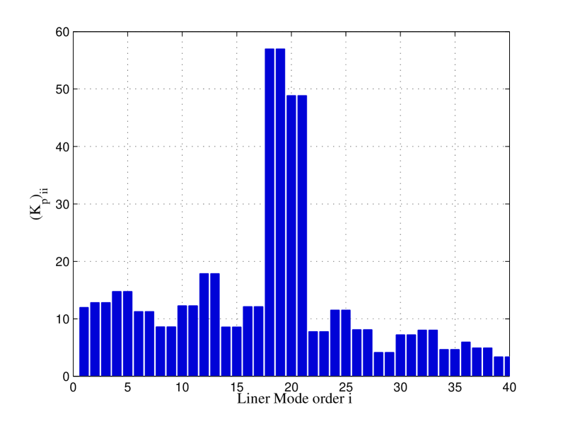
Figure 2: $K_{ii}$ for $R_{l}=1.26$. $i=18-21$ corresponds to the liner modes (9, 1) cosine component, (9, 1) sine component, (9, 0) cosine component, (9, 0) sine component.

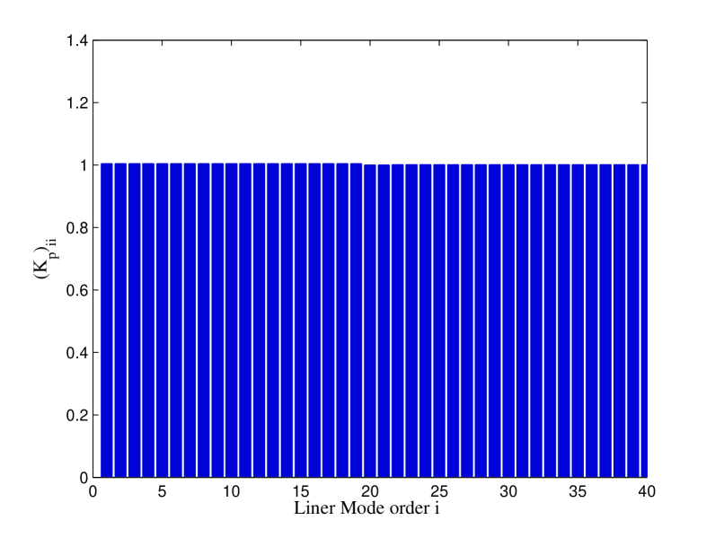
Figure 3: $K_{ii}$ for $R_{l}=0.02$. $i=18-21$ corresponds to the liner modes (9, 0) cosine component, (9, 0) sine component, (9, 1) cosine component, (9, 1) sine component.

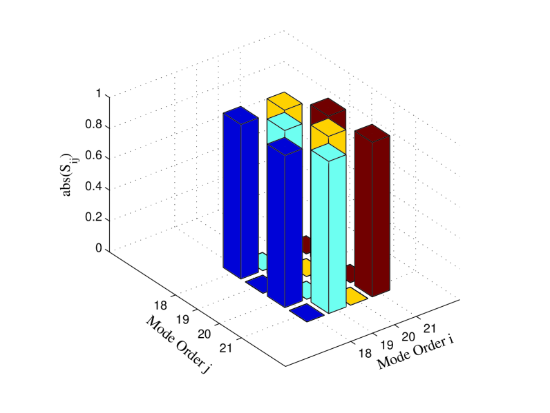
Figure 4: $S_{ij}$ for $R_{l}=1.26$. Mode order $i,j$ is same as in Figs. (3), (3).

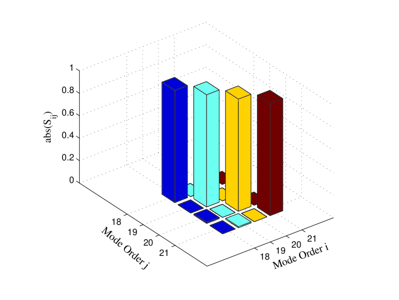
Figure 5: $S_{ii}$ for $R_{l}=0.02$. Mode order $i,j$ is same as in Figs. (3), (3).

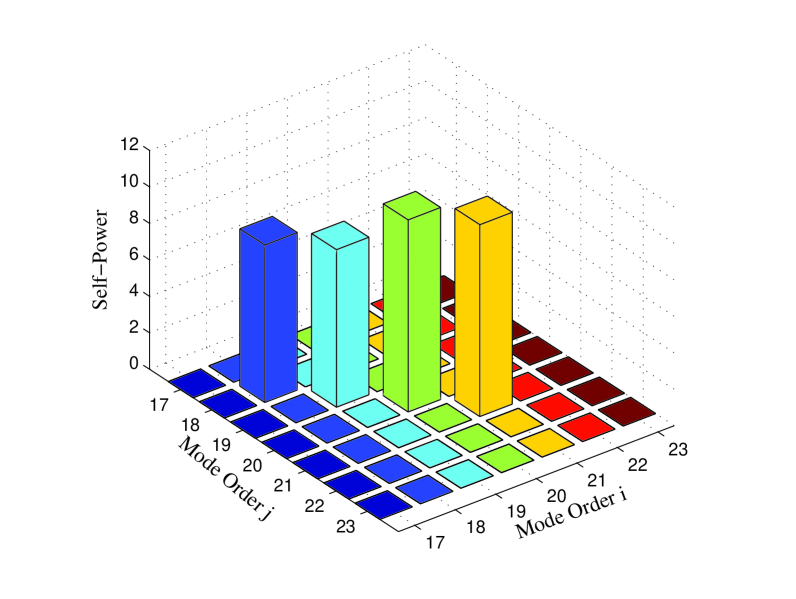
Figure 6: Self-power for $R_{l}=1.26$. Mode order $i,j$ is same as in Figs. (3), (3).

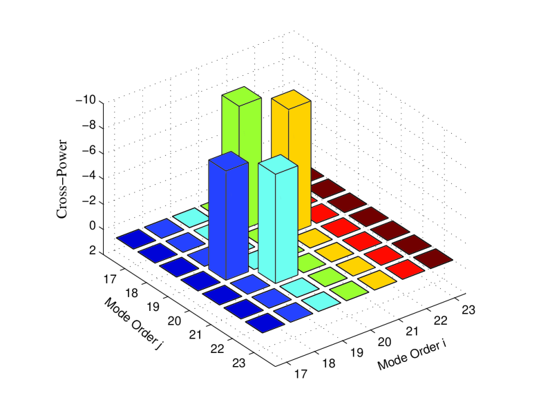
Figure 7: Cross-power for $R_{l}=1.26$. Mode order $i,j$ is same as in Figs. (3), (3).

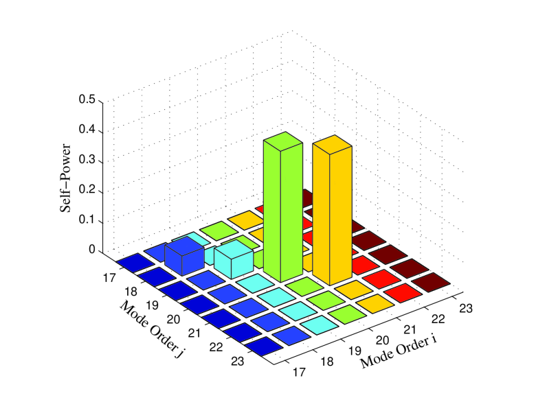
Figure 8: Self-power for $R_{l}=0.02$. Mode order $i,j$ is same as in Figs. (3), (3).

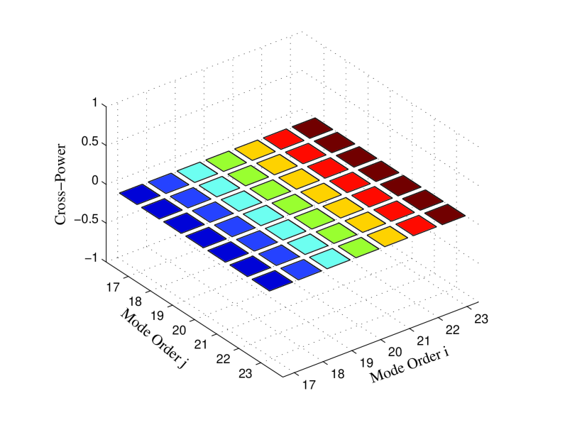
Figure 9: Cross-power for $R_{l}=0.02$. Mode order $i,j$ is same as in Figs. (3), (3).

We will compare two cases $R_{l}=1.26$ and $R_{l}=0.02$ for $K=15.05$. In Figs. (3-9), we plot $K_{ii}$, $S_{ij}$, self-power and cross-power for liner mode (9, 0) and (9, 1). Mode indices $i=18-21$ refers to the liner modes (9, 1) cosine component, (9, 1) sine component, (9, 0) cosine component, (9, 0) sine component for $R_{l}=1.26$. Mode indices $i=18-21$ corresponds to the liner modes (9, 0) cosine component, (9, 0) sine component, (9, 1) cosine component, (9, 1) sine component for $R_{l}=0.02$.

When $R_{l}=0.02$, lining impedance is nearly purely reactive including a very small absorption. The left eigenfunctions of modes (9, 0) and (9, 1) are approximately equal to their right eigenfunctions. All $K_{ii}$ are nearly equal to 1 as shown by eq. (22) and Fig. (3). Modes (9, 0) and (9, 1) are approximately orthogonal under the standard definition (1), $S_{ii}=1$ and $S_{ij}\approx 0$ when $i\neq j$. The total sound power is approximately equal to the sum of the each self-power, i. e., the sum of the sound power of modes (9, 0) and (9, 1). The cross-power between modes (9, 0) and (9, 1) are approximately equal to zero as shown in Fig. (9).

On the other hand, When $R_{l}=1.26$, lining impedance is in the vicinity of optimum impedance of modes (9, 0) and (9, 1). The left eigenfunctions of modes (9, 0) and (9, 1) are equal to the complex conjugate of their right eigenfunctions. $K_{(9,0),(9,0)}=49$ and $K_{(9,1),(9,1)}=57$ as shown Fig. (3). Modes (9, 0) and (9, 1) are bi-orthogonal under the modified definition (2). Modes (9, 0) and (9, 1) are highly similar in the sense of eq. (22). $S_{ij}\approx 1$, where $i,j$ refer to (9, 0) and (9, 1) respectively. The total sound power is not equal to the sum of the self-power, i. e., the sound power of modes (9, 0) and (9, 1). The cross-power between modes (9, 0) and (9, 1) are very important as shown in Fig. (7) (attention: in Fig. (7), the cross-power is negative). The negative cross-power highly destroy the effects of optimum attenuation of each mode.

4 Conclusions

In this paper, we propose two new physical quantities $\mathsf{K_{p}}$ and $\mathsf{S}$. $(K_{p})_{ii}$ describe the self-overlap of the left eigenfunction and right eigenfunction of one mode. $S_{ij}$ ($i\neq j$, $S_{ii}=1$) describe the normalized overlap between modes. The two new physical quantities describe totally the mode behavior in lined ducts.

In the two extreme cases are: When the boundary is acoustic rigid, left eigenfunction is equal to the right eigenfunction, $(K_{p})_{ii}=1$; Modes are mutual orthogonal in the standard definition (1), $S_{ij}=0$ ($i\neq j$). At optimum impedance, $(K_{p})_{ii}=\infty$, left eigenfunction and right eigenfunction are self-orthogonal; $S_{ij}=1$ ($i\neq j$), two modes coalescence. In all other lining impedance cases, $1\leq(K_{p})_{ii}<\infty$ and $0\leq S_{ij}\leq 1$ ($i\neq j$).

We have shown that $\mathsf{K_{p}}$ and $\mathsf{S}$ play essential roles in the sound propagation and attenuation in lined parts. We believe that our results are important in understanding the optimum design of liners.

References

- [1] L. Cremer, Theory of sound attenuation in a rectangular duct with an absorbing wall and the resultant maximum attenuation coefficient, (in german) Acustica 2, 249-263 (1953).
- [2] B. J. Tester, The optimization of modal sound attenuation in duct, in the absence of mean flow, J. Sound Vib. 27, 477-513, (1973).
- [3] B. J. Tester, The propagation and attenuation of sound in lined ducts containing uniform or ”plug” flow, J. Sound Vib. 28, 151-203, (1973).
- [4] E. L. Shenderov, Helmholtz equation solutions corresponding to multiple roots of the dispersion equation for a waveguide with impedance walls, Acoustical Physics, 46, 357-363, (2000).
- [5] J.F. Unruh, Finite length tuning for low-frequency lining design, J. Sound and Vib., 45, 5-14 (1976).
- [6] W.R. Watson, Circumferentially segmented duct liners optimized for axisymmetric and standing-wave sources, NASA-2075 (1982).
- [7] C. R. Fuller, Propagation and radiation of sound from flanged circular ducts with circumferentially varying wall admittances, I: semi-infinte ducts, J. Sound and Vib., 93, 321-340 (1984).
- [8] B. Regan, J. Eaton, Modeling the influence of acoustic liner non-uniformities on duct modes, J. Sound and Vib., 219, 859-879 (1999).
- [9] R. Mani, Acoustic duct with peripherally segmented acoustic treatment, US Patent 3937590 (1976).
- [10] W. P. Bi, V. Pagneux, D. Lafarge, and Y. Aurégan, Modelling of sound propagation in a non-uniform lined duct using a multi-modal propagation method, J. Sound and Vib., 289, 1091-1111 (2006).
- [11] C. K. Tam et al, Scattering of acoustic duct modes by axial liner splices, J. Sound and Vib., 310, 1014-1035 (2008) .
- [12] B. Tester, N. Baker, A. Kempton, and M. Wright, Validation of an analytical model for scattering by intake liner splices, AIAA Pap. 2004-2906, (2004).
- [13] Elnady, T., and Boden, H., Hard Strips in Lined Ducts, AIAA Pap. 2002-2444, (2002).
- [14] E. R. Rademaker, S. L. Sarin, and C. A. Parente, Experimental investigation on the influence of liner non-uniformities on prevailing modes, AIAA Pap. 96-1682 (1996).
- [15] W. P. Bi, V. Pagneux, D. Lafarge, and Y. Aurégan, An improved multimodal method for sound propagation in non-uniform lined ducts, J. Acoust. Soc. Am. 122, 280-291 (2007).
- [16] W. P. Bi, Calculations of modes in circumferentially nonuniform lined ducts, J. Acoust. Soc. Am. 123, 2603-2612 (2008).